DOI:10.32604/iasc.2022.021583
| Intelligent Automation & Soft Computing DOI:10.32604/iasc.2022.021583 | |
| Article |
Target Classification of Marine Debris Using Deep Learning
1Bahria University, Islamabad, Pakistan
2Bahria University, Karachi, Pakistan
*Corresponding Author: Samabia Tehsin. Email: stehseen.buic@bahria.edu.pk
Received: 07 July 2021; Accepted: 12 August 2021
Abstract: Marine Debris is human-created waste dumped into the sea or ocean. It pollutes the aquatic environment and hence very dangerous for ocean species. Removal of marine debris from ocean is necessary to eliminate pollution and to secure aquatic life. A robust and automatic system is essential that detects unnecessary litter of plastic and other garbage at real-time. In this study, we have proposed deep learning based architecture for the detection and classification of marine debris. Histogram Equalization technique combined with Median Filter is used to enhance the contrast of images and to remove noise. Experiments are performed on challenging Forward Looking Sonar Image (FLS) Marine Debris Dataset. This dataset includes ten different types of Debris. The proposed system not only detect the Debris, but also classify it into ten classes. To overcome the challenge of data scarcity, Faster-RCNN with transfer learning of ResNet-50 architecture is used. Faster-RCNN is one of the popular object detection architecture that uses Regional Proposal Network (RPN) and detector at the same time. The proposed methodology significantly improves the state-of-the-art results. Result assessment of our proposed technique achieved recall of (96%) and Mean Overlap bounding boxes of (3.78). Visual and qualitative assessment of proposed methodology shows the effectiveness of presented technique.
Keywords: Marine debris; target classification; deep learning
Due to increase in human population, there is a significant need to increase the production of goods. For this purpose, various industries have been built to produce goods in bulk. But these industries are polluting the environment in different ways. Many processed materials take many years to completely decompose, like heavy metals, plastics, rubbers etc. Man-made garbage is the key factor in environmental pollution. This pollution is degrading the health of land and aquatic living-beings. Now a days, access to pure air and water is a challenging task. Many efforts are done to lessen the effects of pollution on humans and animals; such as recycle and reuse of products, anti-litter campaigns etc. [1].
The amount of garbage is increasing dramatically around the globe and this is big threat for marine creatures. The proper management is required for collection of waste material and litters. In the marine environment the most abominated aspect is the assortment of waste from the streets, roads or beaches, and leaked oil from factories. It is very difficult to remove these waste materials manually from water reservoirs. Autonomous vehicles can be a good option for such removal. Detection and classification of Debris is most challenging part for such autonomous machines.
Most of the man-made garbage is floating on the water surface, some of the garbage collected in the water column and rest is sunk to the bottom of the ocean, these types of garbage are known as debris. This is the major challenge for marine wildlife and habitats as the debris is spoiling the marine life.
Debris comprises of a wide variety of items including rubber, plastic, glass, juice cans, polystyrene, polyethylene, wood, heavy metal, paper, cardboard, discarded ropes, etc. In 2008, Sheavly et.al [1] estimated that 80% of debris is entering in the ocean every year through multiple resources like seashore tourism, factories spilled polluted oil & carbonated water, sewerage & sanitary lines, storm water, wind, etc. According to the survey of Marcus et.al in 2014 the plastic debris is more than 250,000 Tons [2]. According to survey in [3], on average 13000 pieces of debris are floating on the surface water. Fig. 1 shows the distribution of marine debris.
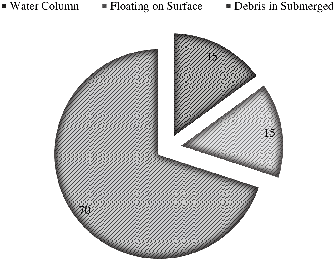
Figure 1: Distribution of debris
Volunteers, nongovernmental organizations, and local governments employed some efforts to capture or remove marine debris, but overall these efforts are insufficient and not at large scale. As a result, the amount of marine debris is increasing drastically every year. Without a well-organized mechanism for debris removal, marine life may extinct. It is a globally recognized ecological issue as it possesses a big threat to the native marine wildlife. Most of the pollution causing items cannot dissolve in the water and stays for the long time at the bottom of a water body [4] . It is also an alarming fact that the debris is growing exponentially every annum [5]. Few examples of Debris are presented in Fig. 2.
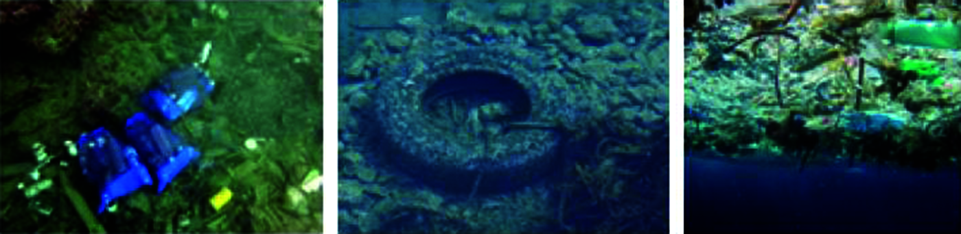
Figure 2: Sample images of debris
Well organized automation system for Debris identification and cleaning is the need of the hour. There are different methods applied for the removal of different types of Debris. So the very first and trivial phase of this automation is identification and classification of Debris in water. This research is focusing on the aforesaid phase.
Sonar images are mostly used for the underwater imagery. Sonar images are grey tone images with no-color information. The proposed study deals with the detection of debris in Sonar images by specifying the precise location for removal. This study also covers the classification of Debris for effective removal of Debris from water.
In this section, studies related to detection and recognition, are reviewed. Many methods are deployed for the detection of Debris in underwater images [6–8]. These methods can be categorized in two classes; conventional Machine Learning based methods and Deep Learning based methods.
2.1 Traditional Machine Learning Techniques
There are many techniques to detect the objects in sonar images. One of the technique is template matching, in which template and query images are compared, cross-correlation is computed [9] and maximum correlation is used for matching [10].
Hurtós et.al. [9] proposed the framework of chain link detection. In first step, images were enhanced using Fourier transformation, then pattern recognition is achieved using clustering method. This solution can only be applied for the inspection and cleaning of the mooring chains using an autonomous underwater vehicle equipped with a forward-looking sonar. For the best results, authors applied algorithm on three different FLS datasets, with detection accuracy of 84%, 92% and 62% respectively.
Haar-boosted cascade framework was first introduced in 2001 by Viola et al. [11]. It is then refined by different researchers and used in different applications, including underwater imagery [12,13]. It gained a lot of attention because of high detection rate and speed.
For the semi-automatic recognition of marine debris on a seashore, light detection and ranging (LIDAR) technique is proposed by Ge et al. in 2016 [14]. The technique is much efficient and reduced the laborious work. LIDAR is mainly used for the classification of marine debris. But it only considered few classes of debris. This technique uses 3-dimensional models for detection of laser scanned images. Support Vector Machine is used for classification.
2.2 Deep Learning Based Techniques
The traditional neural networks were used for Debris detection, which gave low detection rates. In [15] the author focuses on marine debris classification by using two stack of Convolution neural network to classify the image of size 96*96 and gets the accuracy of 70.8%.
Toro [16] proposed the use of Autonomous Underwater Vehicles to detect submerged marine debris from Forward-Looking Sonar (FLS) imagery. Valdenegro-Toro learned the object features by using convolution neural network. This work uses Forward-Looking sonar (non-color) images in-house dataset and therefore computational cost is very high. This method achieves the accuracy of 95% with 3.24 mean IoU.
There is a rich literature about marine debris pollution in the environment. Laist [17] mentioned the effects of plastic garbage on marine environment. The report explains the process of plastic break down by sunlight . It also elaborates the effects of ingestion of these plastic particles on digestive tracts of marine animals. It is also a major cause of death of micro-organism. Discarded fishing nets that are made by polystyrene material can trap animals, causing those drown or be preyed by predators [18–20].
Kylili et al. [21] proposes neural network architecture with very small convolutional layers. This research reported an accuracy of 86%. In this research marine plastic debris image classification is addressed that distinguishes between three classes of litter; plastic bottles, plastic buckets and plastic straws.
In Fulton et al. [22] developed a dataset of colored images named as J-EDI (JAMSTEC E-library of Deep-sea Images). This dataset is developed by including images from three different oceans. Different deep neural networks are also used for the detection of marine debris [23].
A limited number of studies have been performed on Marine debris detection and classification. Various traditional machine learning and deep learning based techniques have been used which gave competitive results, but used a small dataset. Moreover, most of the methods are class-independent and some are class-agnostic. The class-agnostic methods performance is not up to the mark which can be improved. Moreover, classification should be added with localization and detection. So it can be used for autonomous cleaning.
This research proposes a methodology for detection, localization and classification of Debris. It also provides data cleaning to deal with the poor quality images.
Faster-RCNN is adapted for the problem under the study. Faster-RCNN is one of the popular object detection architecture that uses Regional Proposal Network (RPN) and Detector at the same time. The RPN with the help of selective search and edge boxes, produces inexpensive features than the state of the art algorithms. Fig. 3 explains the proposed methodology in detail.
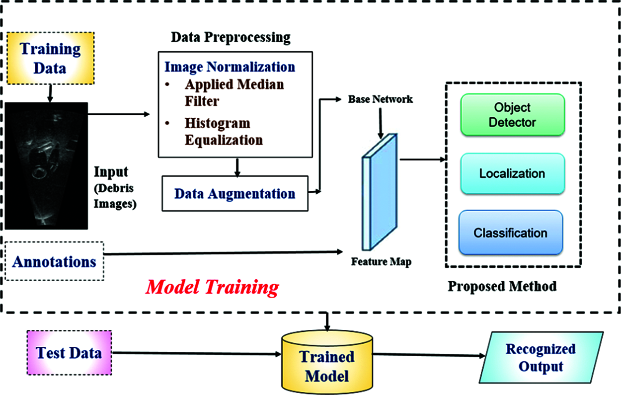
Figure 3: Proposed methodology
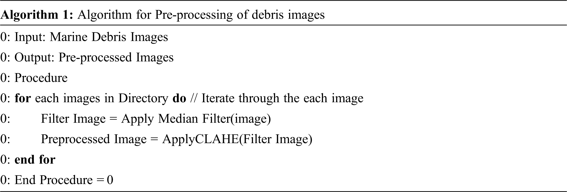
Images in the dataset contains noise because of impurities and water. Due to low light travel under the water, the pictures contains noise. Median filter and histogram equalization is applied to remove this noise [24]. The algorithm of pre-processing is shown in Algorithm 1. Proposed pre-processing technique improves the performance of localization and classification task.
Data augmentation is used to generate more data for training, hence improves performance [25]. Following transformations have been done on training data to increase the size of data:
• Flip by 90°
• Horizontal rotate
• Vertical rotate
This will increase the size of training dataset three times. That will help in better training of proposed model.
3.3 Features Extraction and Classification
Proposed model divides the image into several regions. Features are extracted for each region. The extracted features from each region are then given to the Region Proposal Network (RPN). Faster R-CNN, presented in 2015, is used for classification [26]. It is the third revision of R-CNN architecture. The RCNN uses selective search to find possible region of interest and CNN is used to classify regions [27]. In Fast RCNN a technique called Region of Interest (RoI) pooling is used to make the model fast [26]. Faster RCNN uses Region Proposal Network (RPN).
The architecture of Faster RCNN and proposed methodology is shown in Fig. 4. It will take input image which is passed to the pre-trained model to extract features. Using transfer learning for feature extraction is a common practice used in different computer vision tasks. This will solve the issue of data scarcity and improves the performance of system.
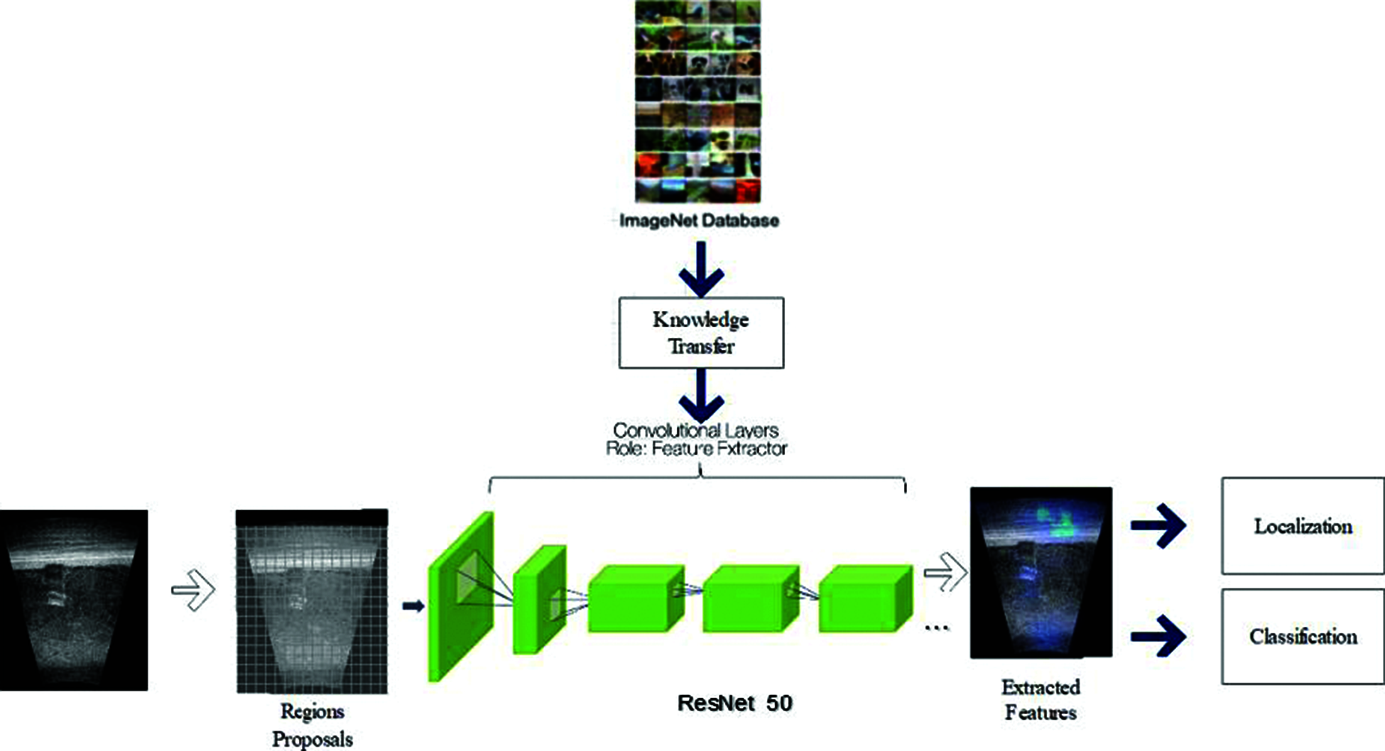
Figure 4: Features extraction and classification
After this, RPN uses the extracted features to find predefined regions which contains objects. One of difficult task in deep learning is to generate variable number of bounding boxes. To solve this issues, anchor boxes are used. These anchors are placed in the images uniformly. Instead of detecting objects in images, the problem is solved in two phases. First, content of bounding box is classified and then the bounding boxes co-ordinates are adjusted.
Standard Faster-RCNN used VGG-16 architecture, but other architectures can also be used. In this study, we have used VGG-16 and ResNet-50 architectures, both are pre-trained on ImageNet [28]. The advantage of using ResNet-50 over VGG16 is that this architecture is big and have the capacity to learn more features.
While working on images, the aim is to find proposals (regions with area of interest). Proposal is an area of interest with fixed predefined bounding boxes. These are placed in all image points at specified ratio to predict object location. There are 9 anchor boxes for each point of image in the feature map, with aspect ratio 1:1, 1:2 and 2:2. Anchor boxes are shown in Fig. 5.
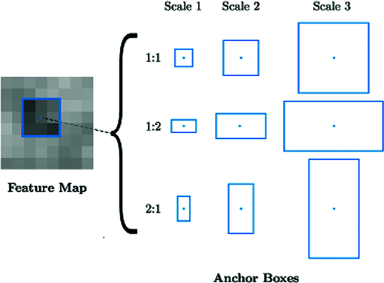
Figure 5: Anchors with aspect ratio 1:1 1:2 2:2
R-CNN is final step in Faster-RCNN. Feature maps from RPN is used for the classification. The aim of RCNN is to classify the proposals into classes and adjust the bounding box. Faster RCNN can be optimized by using multi-task loss function. This loss function is the combination of classification loss and bounding boxes loss.
where pi is the probability of anchor as a class,
Lcls is the log loss function over two classes which can be extended to multi-class problem and
Lreg is operational when anchor got object, when ground truth
Here x, y, w, and h correspond to the coordinates of the box center, width and height. xa and
At test time, the learned regression output ti can be applied to its corresponding anchor box (that is predicted positive), and the x, y, w, h parameters for the predicted object proposal bounding box can be calculated by following equations.
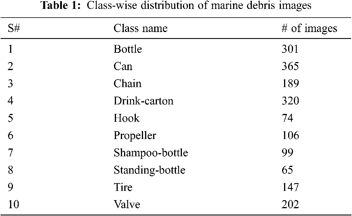
We have used Forward Looking Sonar Image (FLS) Marine Debris Dataset. These images are captured at OCEAN SYSTEM Lab Water Tank at Heriot-Watt University. These are captured by ARIS Explorer 3000 with setting of 3.0 MHz frequency. This dataset is labeled with bounding boxes annotations and images are manually cropped. It consists of 10 classes with 1865 images.
The Marine Debris Forward-Looking Sonar (FLS) Dataset contained non-colored images. Included classes are bottle, can, chain, drink can, hook, propeller, shampoo bottle, standing bottle, tire, and valve. The size of Marine Debris-FLS is 362 MB. Tab. 1 shows class wise distribution of images in the dataset.
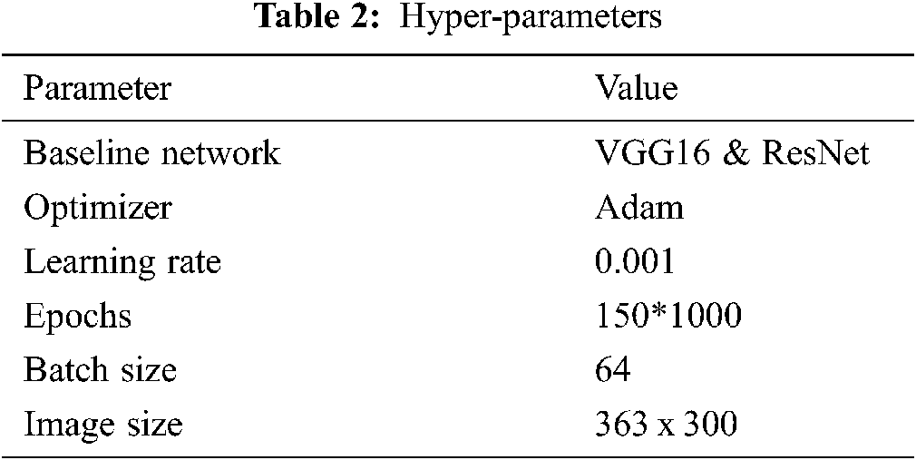
The experimental settings used to perform this study are listed in Tab. 2. We have used the baseline networks as VGG16 and ResNet. Adam optimizer is used with learning rate of 0.001. The network is run with 150 epochs and batch size of 64. The experiments are performed on Google Colab platform having 16 GB ram and 12 GB GPU memory.
For the assessment of proposed methodology, we have used recall, Mean IoU and accuracy. For localization Mean IoU is used. IoU measures the location similarity of two regions. It is defined as:
where A and B are two bounding boxes, A is the actual bounding box and B is the predicted one. Accuracy is defined as the measure to find how correctly the predictions are identified.
where TP is true positive, TN is true negative, FP is False positive and FN is False negative.
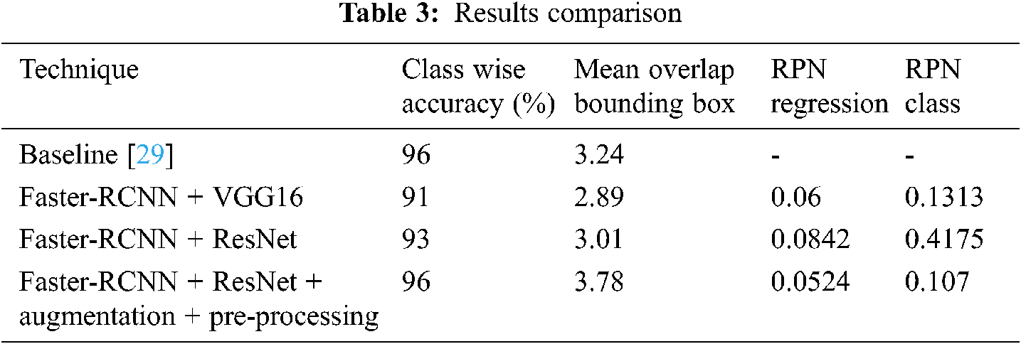
We have compared our results of our proposed architecture with the baseline architecture. Therefore, we have conducted experiments and compared our proposed technique with baseline FCN architecture. We have used VGG16 and ResNet architectures, pre-trained on ImageNet datset. The baseline method proposed a class agnostic object detector. The Tab. 3 shows the results comparison of baseline approach with Faster RCNN.. The baseline architecture is computationally expensive as features are not shared across neural network evaluations, and simple threshold of objectness values might not generalize well across environments. Whereas, Faster-RCNN uses RPN which uses the divide and conquer strategy. In RPN the regions are divided into multiple proposals and then features are extracted and object along with the bounding box is detected. The RPN adjust the bounding region with the predicted objects as it is class-aware whereas, the baseline architecture fails to do so. By using augmentation and pre-processing with Faster-RCNN with Resnet achieves, class-wise accuracy of 95% and mean IoU of 3.74. The proposed approach outperform the baseline technique in terms of Mean IoU and class-wise accuracy.
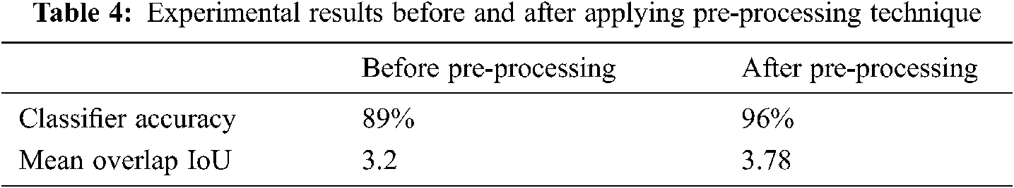
The Tab. 4 shows the experimental results before and after applying the preprocessing techniques. Some of the regions in the debris sonic images are unclear due to noise and distortion. Low light is the main reason of image noise. Applying pre-processing technique improves the contrast of image in sonar scans. After applying proposed preprocessing mechanism, Mean- IoU is increased from 3.2 to 3.78 and accuracy improves from 89% to 95%. Fig. 6 shows the learning curves of total loss, Mean IoU and class-wise accuracy using VGG16 with Faster-RCNN architecture. The learning curves for ResNet architecture is shown in Fig. 7.
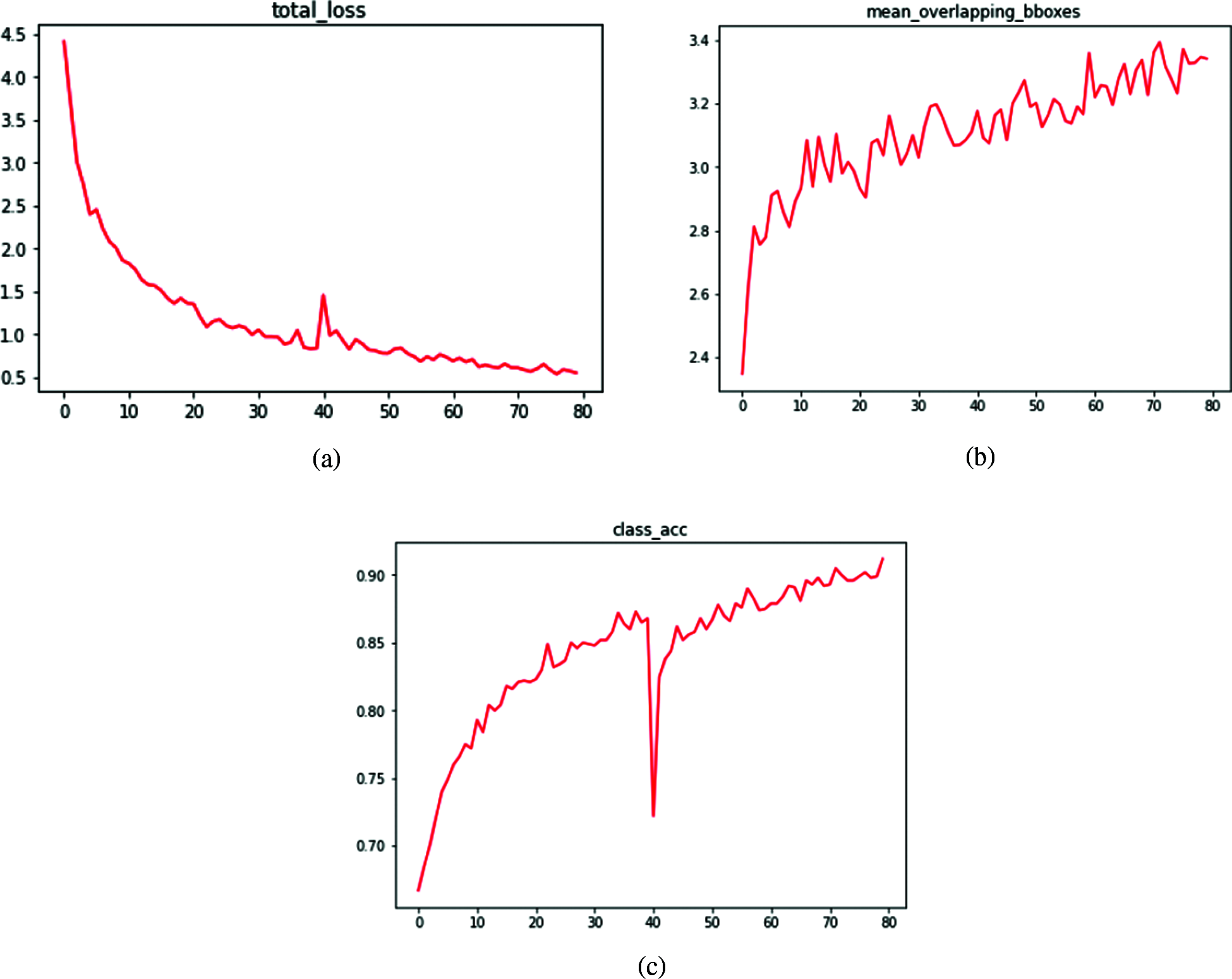
Figure 6: Learning curves of faster–RCNN + VGG16 (a) loss (b) mean overlapping IoU (c) classwise accuracy
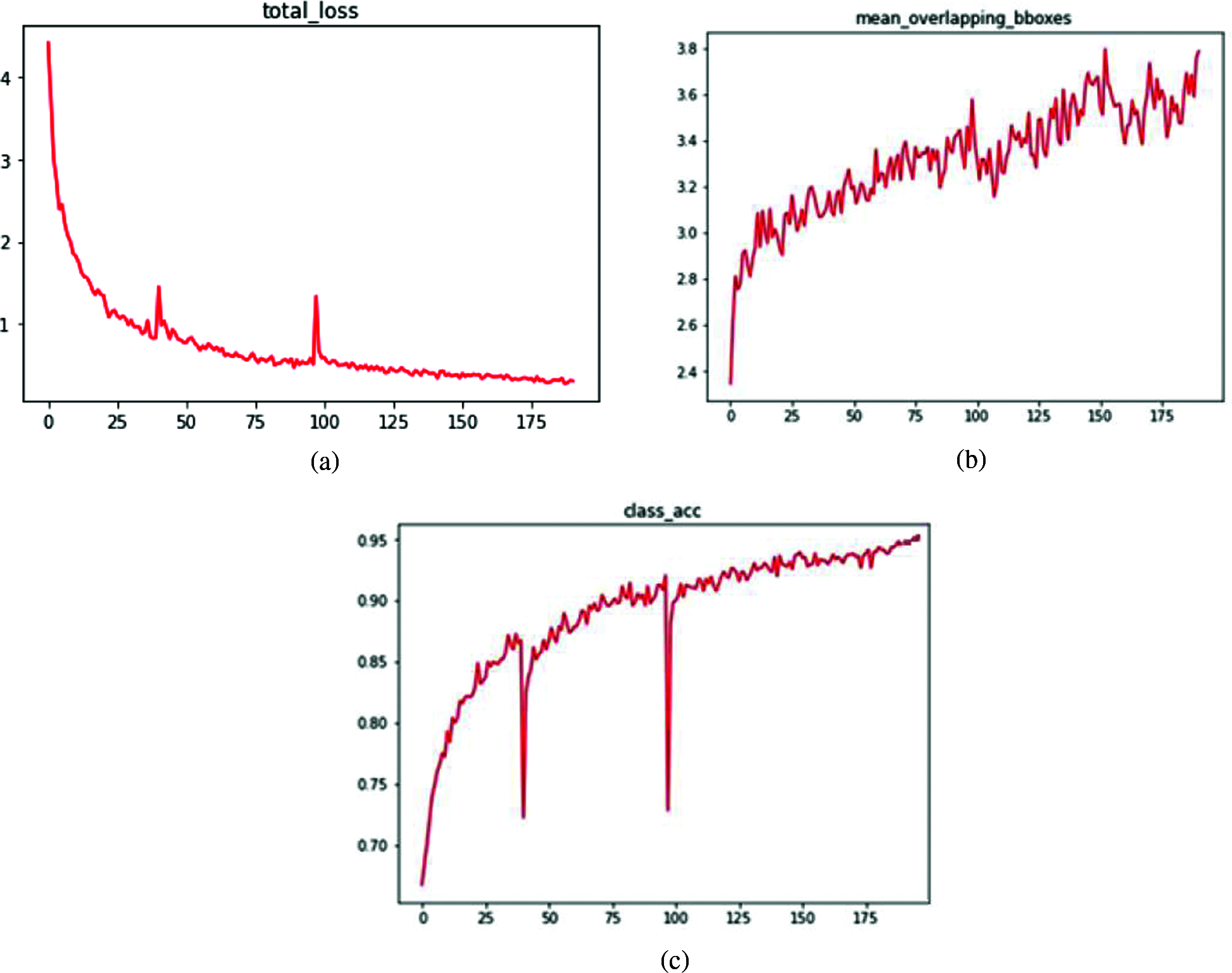
Figure 7: Learning curves of faster–RCNN + ResNet 50 (a) loss (b) mean overlapping IoU (c) classwise accuracy
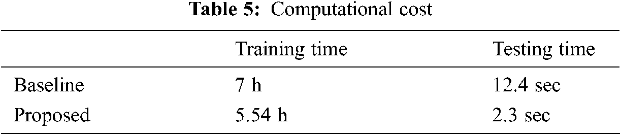
We have compared the proposed architecture with baseline architecture in terms of computational time and complexity. 70% Data is used for training whereas 30% data is used for testing. Comparison is reported in Tab. 5.
A methodology for detection of marine debris images is proposed using Faster-RCNN with ResNet 50. An effective preprocessing methodology is also proposed to enhance the performance. Experimental results shows improvement after pre-processing technique.
We have performed experiments on challenging marine debris detection. To overcome the challenges of data scarcity and Debris classification, Faster RCNN architecture with transfer learning of baseline architectures (VGG16 & ResNet) is used. The proposed methodology significantly achieves competitive results as compared to previous studies.
The microplastic is also a big threat to the wildlife of marine. It can be addressed in future research. Ensemble technique may also be addressed as future work for performance improvement.
Funding Statement: The authors received no specific funding for this study.
Conflicts of Interest: The authors declare that they have no conflicts of interest to report regarding the present study.
1. S. B. Sheavly and K. M. Register, “Marine debris & plastics: Environmental concerns, sources, impacts and solutions,” Journal of Polymers and the Environment, vol. 15, no. 4, pp. 301–305, 2007. [Google Scholar]
2. M. Eriksen, L. Lebreton, H. Carson, M. Thiel, C. J. Moore et al., “Plastic pollution in the world’s oceans: More than 5 trillion plastic pieces weighing over 250,000 tons afloat at sea,” PLOS One, vol. 9, no. 12, pp. e111913, 2014. [Google Scholar]
3. G. Pasternak, D. Zviely, C. A. Ribic, A. Ariel and E. Spanier, “Sources, composition and spatial distribution of marine debris along the Mediterranean coast of Israel,” Marine Pollution Bulletin, vol. 114, no. 2, pp. 1036–1045, 2017. [Google Scholar]
4. E. V. Sebille, S. Aliani, K. L. Law, N. Maximenko, J. M. Alsina et al., “The physical oceanography of the transport of floating marine debris,” Environmental Research Letters, vol. 15, no. 2, pp. 23003 2020. [Google Scholar]
5. J. Sawas and Y. Petillot, “Cascade of boosted classifiers for automatic target recognition in synthetic aperture sonar imagery,” in Proc. Meetings on Acoustics ECUA2012, vol. 17, no. 1, pp. 70074, 2012. [Google Scholar]
6. L. Ma, H. Shi, H. Zhang, G. Li, Y. Shen et al., “High-sensitivity distinguishing and detection method for wear debris in oil of marine machinery,” Ocean Engineering, vol. 215, pp. 107452, 2020. [Google Scholar]
7. A. Antti, M. Kiviranta and M. Höyhtyä, “Space debris detection over intersatellite communication signals,” Acta Astronautica, vol. 187, pp. 156–166, 2021. [Google Scholar]
8. D. Dvoryankov, D. Valuyskiy, S. Vityazev and V. Vityazev, “The problem of debris detection with automotive 77-gHz FMCW radar,” in Proc. IEEE 10th Mediterranean Conf. on Embedded Computing (MECOMontenegro, pp. 1–4, 2021. [Google Scholar]
9. N. Hurtós, N. Palomeras, S. Nagappa and J. Salvi, “Automatic detection of underwater chain links using a forward-looking sonar,” in Proc. MTS/IEEE OCEANS-Bergen, Norway, pp. 1–7, 2013. [Google Scholar]
10. T. A.Ruz, D. Uribe, R. Taylor, L. Amézquita, M. C. Guzmán et al., “Anthropogenic marine debris over beaches: Spectral characterization for remote sensing applications,” Remote Sensing of Environment, vol. 217, pp. 309–322, 2018. [Google Scholar]
11. P. Viola and M. Jones, “Rapid object detection using a boosted cascade of simple features,” in Proc. IEEE Computer Society Conf. on Computer Vision and Pattern Recognition, USA, pp. I–I, 2001. [Google Scholar]
12. R. Lienhart and J. Maydt, “An extended set of haar-like features for rapid object detection,” in Proc. Int. Conference on Image Processing, USA, pp. I–I, 2002. [Google Scholar]
13. R. Lienhart, A. Kuranov and V. Pisarevsky, “Empirical analysis of detection cascades of boosted classifiers for rapid object detection,” in Joint Pattern Recognition Symp., Germany, pp. 297–304, 2003. [Google Scholar]
14. Z. Ge, H. Shi, X. Mei, Z. Dai and D. Li, “Semi-automatic recognition of marine debris on beaches,” Scientific Reports, vol. 6, no. 1, pp. 1–9, 2016. [Google Scholar]
15. L. Sherwood, “Applying Object Detection to Monitoring Marine Debris,” Ph.D. dissertation, University of Hawaii at Hilo, 2020. [Google Scholar]
16. M. V. Toro, “Submerged marine debris detection with autonomous underwater vehicles,” in Proc. Int. Conf. on Robotics and Automation for Humanitarian Applications (RAHAIndia, pp. 1–7, 2016. [Google Scholar]
17. D. W. Laist, “Overview of the biological effects of lost and discarded plastic debris in the marine environment,” Marine Pollution Bulletin, vol. 18, no. 6, pp. 319–326, 1987. [Google Scholar]
18. P. G. Ryan, “A simple technique for counting marine debris at sea reveals steep litter gradients between the straits of malacca and the Bay of Bengal,” Marine Pollution Bulletin, vol. 69, no. 1–2, pp. 128–136, 2013. [Google Scholar]
19. J. P. Harrison, J. J. Ojeda and M. E. González, “The applicability of reflectance micro-Fourier-transform infrared spectroscopy for the detection of synthetic microplastics in marine sediments,” Science of the Total Environment, vol. 416, pp. 455–463, 2012. [Google Scholar]
20. J. R. Jambeck and K. Johnsen, “Citizen-based litter and marine debris data collection and mapping,” Computing in Science & Engineering, vol. 17, no. 4, pp. 20–26, 2015. [Google Scholar]
21. K. Kylili, I. Kyriakides, A. Artusi and C. Hadjistassou, “Identifying floating plastic marine debris using a deep learning approach,” Environmental Science and Pollution Research, vol. 26, no. 17, pp. 17091–17099, 2019. [Google Scholar]
22. M. Fulton, J. Hong, M. J. Islam and J. Sattar, “Robotic detection of marine litter using deep visual detection models,” in Proc. Int. Conf. on Robotics and Automation (ICRACanada, pp. 5752–5758, 2019. [Google Scholar]
23. I. Marin, S. Mladenović, S. Gotovac and G.Zaharija, “Deep-feature-based approach to marine debris classification,” Applied Sciences, vol. 11, no. 12, pp. 5644, 2021. [Google Scholar]
24. S. M. Pizer, E. P. Amburn, J. D. Austin, R. Cromartie, A. Geselowitz et al., “Adaptive histogram equalization and its variations,” Computer Vision, Graphics, and Image Processing, vol. 39, no. 3, pp. 355–368, 1987. [Google Scholar]
25. D. A. V. Dyk and X. Meng, “The art of data augmentation,” Journal of Computational and Graphical Statistics, vol. 10, no. 1, pp. 1–50, 2001. [Google Scholar]
26. R. Girshick, “Fast r-cnn,” in Proc. IEEE Int. Conf. on Computer Vision, Chile, pp. 1440–1448, 2015. [Google Scholar]
27. K. He, G. Gkioxari, P. Dollár and R. Girshick, “Mask r-cnn,” in Proc. IEEE Int. Conf. on Computer Vision, Italy, pp. 2961–2969, 2017. [Google Scholar]
28. D. Theckedath and R. R. Sedamkar, “Detecting affect states using VGG16, resnet50 and SE-resNet50 networks,” SN Computer Science, vol. 1, no. 2, pp. 1–7, 2020. [Google Scholar]
29. M. V. Tor, “Learning objectness from sonar images for class-independent object detection,” in Proc. European Conf. on Mobile Robots (ECMRCzech Republic, pp. 1–6, 2019. [Google Scholar]
 | This work is licensed under a Creative Commons Attribution 4.0 International License, which permits unrestricted use, distribution, and reproduction in any medium, provided the original work is properly cited. |