DOI:10.32604/iasc.2022.020974
| Intelligent Automation & Soft Computing DOI:10.32604/iasc.2022.020974 | |
| Article |
Optimal Path Planning for Intelligent UAVs Using Graph Convolution Networks
School of Computing, SASTRA Deemed to be University, Thanjavur, 613401, India
*Corresponding Author: P. L. K. Priyadarsini. Email: priya.ayyagari@it.sastra.edu
Received: 16 June 2021; Accepted: 17 July 2021
Abstract: Unmanned Aerial Vehicles (UAVs) are in use for surveillance services in the geographic areas, that are very hard and sometimes not reachable by humans. Nowadays, UAVs are being used as substitutions to manned operations in various applications. The intensive utilization of autonomous UAVs has given rise to many new challenges. One of the vital problems that arise while deploying UAVs in surveillance applications is the Coverage Path Planning(CPP) problem. Given a geographic area, the problem is to find an optimal path/tour for the UAV such that it covers the entire area of interest with minimal tour length. A graph can be constructed from the map of the area under surveillance, using computational geometric techniques. In this work, the Coverage Path Planning problem is posed as a Travelling Salesperson Problem(TSP) on these graphs. The graphs obtained are large in number of vertices and edges and the real-time applications require good computation speed. Hence a model is built using Graph Convolution Network (GCN). The model is effectively trained with different problem instances such as TSP20, TSP50, and TSP100. Results obtained from the Concorde Benchmark Dataset were used to analyze the optimality of the predicted tour length by the GCN. The model is also evaluated against the performance of evolutionary algorithms on several self-constructed graphs. Particle Swarm Optimization, Ant Colony Optimization, and Firefly Algorithm are used to find optimal tours and are compared with GCN. It is found that the proposed GCN framework outperforms these evolutionary algorithms in optimal tour length and also the computation time.
Keywords: Unmanned aerial vehicles; graph convolution networks; travelling salesman problem; graph theory; evolutionary algorithms
As the world is moving towards an era of minimizing the use of human intervention and increasing the usage of autonomous machines, UAVs are not an exception. Autonomous UAVs are being deployed in various applications as their design allows them to visit all the locations where the reach of humans remains impossible or would require more manpower [1–3]. The Coverage Path Planning (CPP) problem is one of the most important challenges that need to be focused upon while deploying a UAV in any real-time surveillance application. Let us consider a scenario where a UAV is deployed to cover all nine locations as shown in Fig. 1. The order in which the UAV opts to maneuver the given set of locations varies and so as the total distance traveled. Two of the alternatives are shown in Figs. 1a and 1b. When UAVs are deployed in disaster management it is very important to find the shortest path very fast, to rescue the human lives at risk. So we need algorithms that find the best solutions in a computationally efficient way.
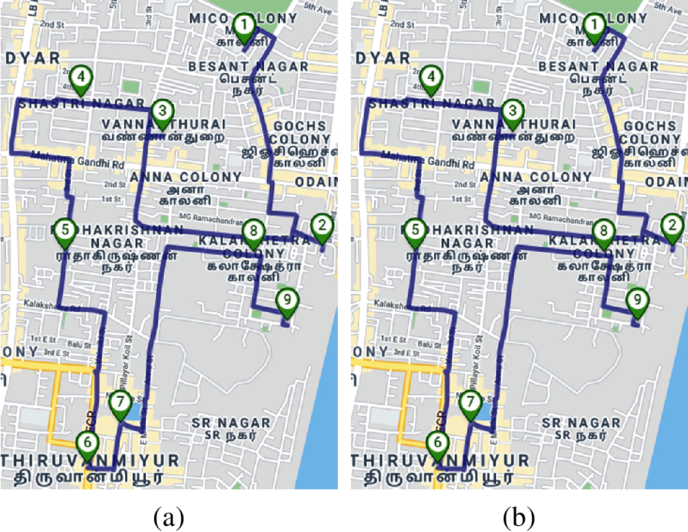
Figure 1: Illustration of possible paths while traversing through UAVs (a) Path 1 (b) Path 2
To find the optimal path for the UAV over a geographic area, we first transform the problem into a graph problem by creating a complete weighted graph from the geographic map given. Let G(V, E) be such a graph with V indicating a set of vertices in the graph and E denoting the set of edges connecting these vertices. Now, the problem can be posed as a TSP, which is one of the most important combinatorial optimization problems. Given a complete weighted graph, the problem is to find a minimum weighted Hamiltonian cycle. Numerous researchers have proposed various ways of solving TSP. As TSP is an NP-complete problem, there are computationally efficient algorithms that produce sub-optimal solutions, proposed in the literature.
This paper assumes that a geographic map is given and an optimal flying path for a UAV, covering the entire area is to be found out. The path of the UAV is to be designed in such a way that it starts at a point and visits each of the given points of coverage once and ends at the same point where it started. In a simple case, the UAV does not face any obstacles such as trees, hilly terrains, and the like. So, the UAV path may be considered to be in a plane. So we can use the boundary of the map to construct a complete graph containing coverage points as vertices. Now the problem will be transformed into finding optimal tour in this graph and it is originally the Travelling Sales Person (TSP) problem.
The use of traditional techniques based on non-learning approaches to find the optimal solution to the TSP problem serves well when the graph size is small. But they are not computationally efficient on large graphs. To overcome this challenge, pre-trained deep learning models can be used to find the solution in real-time, with minimal time.
In this paper, a deep learning framework based on Graph Convolution Network is proposed for finding optimal tours for a given TSP instance. GCNs works the same way as the traditional CNN, but it has the capability of working with the graphs directly by making use of its structural information [4]. They both consider the weighted average of the neighborhood nodes while making a choice. In Fig. 2a, a comparison of calculating the values of nodes by a traditional 2D convolution and Graph convolution is shown. It shows how 2D convolution assumes connections between nodes representing pixels in an image. The value of the green node is determined by taking the weighted average of all its neighboring nodes. Fig. 2b, demonstrates how GCN calculates values of nodes for any given graph. In this, the value of the green node is determined by taking the weighted average of all its adjacent nodes along with their features. GCNs can handle any type of graph structure effectively.
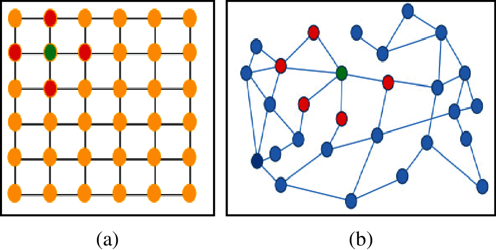
Figure 2: Connection of nodes using distinct methods (a) 2D convolution (b) Graph convolution
The idea behind the usage of GCN is to reduce computation time compared to other techniques including evolutionary algorithms. The framework attempts to obtain an efficient solution with minimal training data. The network is built by training several graphs with solution labels for TSP. TSP Concorde benchmark dataset is used for training purposes. The performance of GCN is compared with that of the other evolutionary techniques. The performances of Particle Swarm Optimization, Ant Colony Optimization, and Firefly Algorithms on graphs of sizes up to 100 nodes, are used for this comparison. The overall architectural diagram of the proposed methodology is shown in Fig. 3.
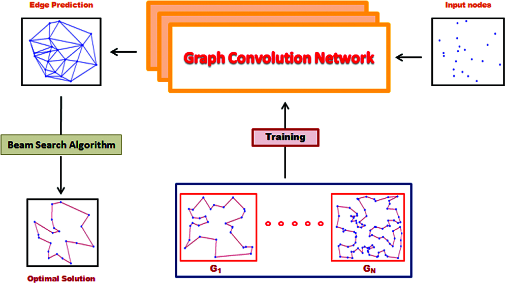
Figure 3: Architectural diagram of the proposed methodology
Initially, the GCN is trained with numerous 2D graphs, G1…GN. After training the model, the network collects the information from the input graph structure with random nodes to output an edge prediction map. This map shows the possible edges between the given input nodes by making use of node features. The final output will be the predicted optimal path by making use of the shortest-heuristic beam search algorithm, over the computed edge prediction graph.
The rest of the paper is organized as follows: Section 2 discusses various works related to the proposed methodology, Section 3 explains the overall proposed methodology of finding an optimal solution for any given graph using GCN. Section 4 provides the results obtained while making use of GCN for 2D Euclidean graphs and is compared with the ground truth to find the optimal gap in the length of the tour obtained. The paper is finally concluded in Section 5 which describes the efficiency of the proposed model when compared with other traditional models and also lists out some future research works.
The use of UAVs in various applications is seeing immense growth and numerous problems related to UAVs are being now researched upon. Deployment of UAVs is nowadays mostly preferred to be in an autonomous way such that it does not need any human intervention. This reduces the manpower and at the same time, it makes it possible to monitor the areas that are out of human reach [5]. Numerous applications are now making use of these autonomous UAVs which in turn need a lot of constraints to be satisfied. Some of the vital problems include area coverage problems, optimal path planning of UAVs, collision avoidance considering both static and dynamic environments.
The major focus of the area coverage problems includes a need where the entire area under coverage needs to be visited. A lot of research works are undergone to traverse the entire area under coverage. The author has presented a rectilinear area partitioning algorithm where the area is divided into multiple rectangular partitions and the centroids of each partition are computed such that visiting that particular centroid will cover the entire rectangle and hence the entire area would be covered by the UAV [6]. CPP problem was stated to be solved using multiple robots [7], by giving effective coverage trajectory for the robots but the details of collision with static and dynamic obstacles have not been mentioned. Identifying the points of interest was stated to be focused in [8], where the Branch and Bound algorithm solved the area coverage problem. Though various algorithms are being proposed for area coverage applications, there remains a necessity of finding an optimal path that needs to be planned for traversing the coverage points in minimal time. The problem can be posed as TSP and various techniques are carried out to solve this problem to find an optimal solution such as ACO, PSO, and Firefly Algorithm. Abdurrahim Sonmez et al. [9] has proposed a genetic algorithm-based optimal path planning for UAVs. The research work claimed to use a 3D environment and the problem was formulated as TSP to find the optimal path.
The TSP was coined in the year 1930 and it is stated to be one of the most studied combinatorial optimization problems. Even though the environment is 2D Euclidean where all the nodes are in two dimensions and the weights between the edges are Euclidean distances, solving TSP is considered to be NP-Hard. TSP solutions can be found by making use of both Non-learning approaches and Learning approaches. Some of the commonly used non-learning approaches include the Nearest approach [10], the Boruvka approach [11], the Lin-Kernighan approach [12], and many more. The major drawback of making use of these approaches is that they fail to handle a large number of data and that the resources used for handling such huge data are always very expensive. The use of machine learning and deep learning techniques can make the work ease by training the policies such that they can solve TSP while making use of large graphs which comprise numerous nodes. The use of Pointer Network(PtrNet) has been suggested by [13] to exclude all the visited nodes in the graph and to find an optimal solution for TSP.
GCN plays a vital role while dealing with graphs. They act similar to CNN but serves better when the network needs to be trained in the graph domain. In the graph domain, the graphs are defined by their vertices, edges, and adjacency matrix whereas the graph features are defined using their node and edge features. The importance of GCN lies in the way on how it learns the information from the graph features. Advances in GCNs can be seen in applications making use of graph structures. Hibiki Taguchi et al. [14] proposed a GCN that could find the missing features in a graph that performed far better than the remaining imputation-based models. Cluster -GCN proposed in Chiang et al. [15], works by exploiting the overall graph clustering structure and has prominently noticed an improvement in the memory and computational efficiency while comparing with the other traditional algorithms. Graph networks seem to work well for solving TSP as the entire problem needs to be solved using graph structures. A Graph-Learning method states that the model had the capability of directly learning the pattern of the TSP datasets during the training time by giving out a very minimal optimality gap [16] but how the output of the GCN might vary in presence of any obstacles is not researched upon. Graph-based convolution networks could be used in applications involving a large number of graphs that need to be processed with near-optimal solutions.
3 Methodology - GCN for Solving TSP
The problem under consideration is to find a path with minimal length traversing through the identified points of coverage. The path needs to cover the entire given geographic area where the UAV is been deployed. The overall problem is formulated to be a TSP for which the solution is to be found by making effective use of GCN. The steps involved in the process include:
• Training the GCN using Benchmark dataset containing optimal solution
• Giving a 2D input graph to the GCN using the Test dataset
• Predicting the edges for the given 2D input graph using feature maps
• Finding the optimal solution using a Heuristic Search Algorithm
• Comparing the optimal tour length obtained from the proposed model with other evolutionary algorithms to find the best technique suitable for the given problem.
In our research work, we have mainly focused on 2D Euclidean TSP, were given an input graph with numerous vertices that will yield an optimal solution. The vertices in the graph represent the sequence of n cities. Generally, all the graphs are two-dimensional in space which gives the coordinates of any two given cities. Graphs from the Concorde dataset include the distance between any two given cities along with their coordinates. Initially, the GCN is trained with a benchmark dataset namely, Concorde TSP whose solutions are obtained using TSP solvers. Fig. 4, shows a sample graph from the Concorde dataset where it gives the optimal tour for the given set of vertices. The blue node depicts the starting and the ending node of the entire tour. The solutions in the dataset are obtained by making use of Concorde Solver. For a given set of random nodes, the Concorde TSP solver can make use of any traditional non-learning approaches present in the state-of-art to obtain a valid tour.
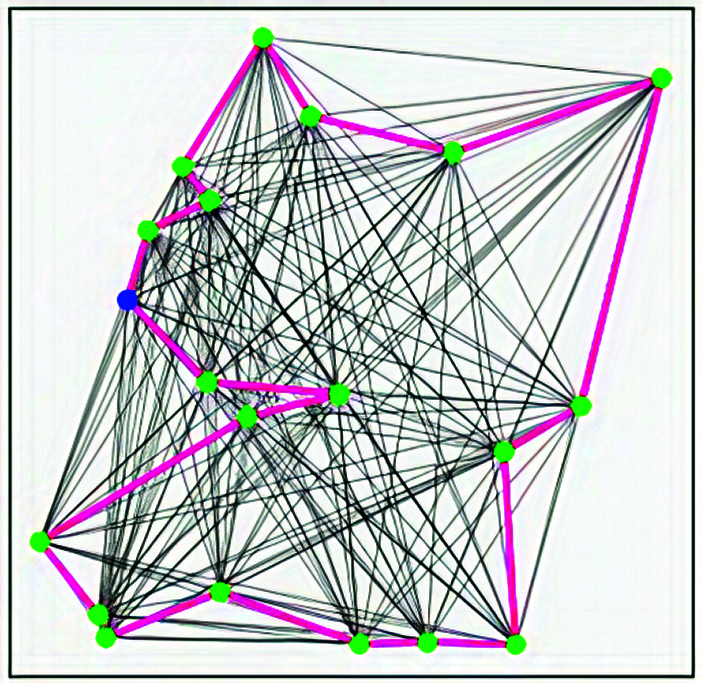
Figure 4: Graph in the concorde dataset
The solutions with optimal tour length are aggregated together to form the Concorde Benchmark dataset. The dataset consists of graphs along with their corresponding TSP tours which help in training the deep learning models. To directly compare with the state of art techniques, the entire dataset is divided into training, validation, and test datasets. The training dataset comprises of 1million pairs of problem instances along with its optimal solutions with graph sizes of 20, 50 and 100. The validation and test dataset comprises 10,000 pairs of problem instances each. The dataset obtained by making use of Concorde solver is used in our proposed work rather than any other TSP solver like Gurobi and LKH3, as Concorde is highly specialized in providing optimal results for 2D Euclidean TSP.
Deep learning allows one to learn very complex and complicated concepts by transforming them into simple forms in a multi-layer fashion. Numerous networks such as convolution networks, recurrent neural networks are used in various applications according to their need. CNN is highly parallelizable and it also scales very well when making use of very large datasets. CNN’s are powerful architectures that are designed to solve problems with high-dimensionality by overcoming the problem of the “curse of dimensionality”. The main assumptions while making use of any convolution networks are that the neurons present in any particular layer are only connected to its adjacent layers and are not connected to all its layers. Some patterns in the data that need to be processed are similar and are shared across the entire domain. The feature at the lower level is combined to form medium-level features which are further combined to form high-level features. They can extract the compositional features from the data which is further used for the classification or prediction process. While considering the data domain, such as sentences and words, they lie on the 1D Euclidean domain. Whereas, when we look into some other types of data such as images and videos they lie on the 2D Euclidean domain. Considering real-time applications such as the ones making use of social networks, the connection between various users forms a graphical representation.
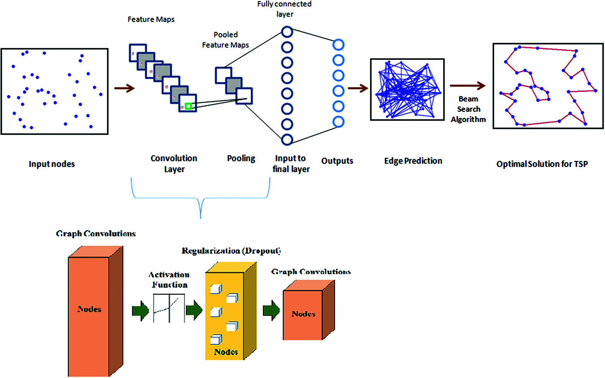
Figure 5: Computation of optimal solution for TSP using GCN
Nowadays, many applications are being incorporated that make use of these graphical representations for processing data. In any graphical representation, Graphs G is defined by its vertices(V), edges(E), and their distance matrix(D) such that G = (V, E, D). These graphs can be processed by making use of GCNs rather than making use of CNNs. The major idea of our proposed work is to approximately solve 2D Euclidean TSP by making use of GCN. In Fig. 5, the entire workflow of our proposed methodology making use of GCN is depicted comprising of the feature maps and the fully connected layer. The GCN effectively outputs an edge prediction map which is further used for finding the optimal tour length for any given graph. In our work, we have made use of GCN that is trained effectively using the TSP dataset such that it predicts the edges for any given graph. It outputs an edge adjacency matrix which denotes the probabilities of edges occurring on the TSP tour. It works similar to that of CNN with a very minimal difference. In CNN, all the images are represented by taking the pixel values as arrays. Whereas in GCN, the graph features such as node and edge level features along with other application-specific features such as the Euclidean distances are used for training purposes.
Feature extraction in graphs can be done at both node level and graph level. One of the easiest methods of capturing information from graphs is to create individual features for each node. These features have the capability of capturing information both from its close neighborhood and also from distant nodes. Feature extraction at the node level includes:
• Node Degree: This is the primary feature extracted which gives the total number of nodes incident on any particular node.
• Eigen Vector Centrality: This feature extraction deals with the importance of any node and also how important the neighbors of that particular node are. Nodes with higher Eigenvector centrality should have many neighbors which are in turn connected to other nodes.
• Clustering Coefficient: This feature answers the question of how tightly groups of nodes are connected. This gives the ratio of the number of edges between the neighbors to the number of node’s neighbors.
Graph level features are used to extract the global information from graphs. One such feature extraction done in our proposed work is the computation of the adjacency matrix which indicates whether pairs of vertices are adjacent or not. Apart from this Neighborhood overlap features are also extracted as node and graph level features fail to gather the information about the relationship between the neighboring nodes. This is one of the most important features that need to be extracted when working with problems about edge prediction tasks. This feature plays a major role in predicting whether there is a connection between two nodes or not by measuring both local and global overlaps in graphs. The input layer extracts various compositional feature vectors from all the available graph nodes by stacking several graph convolution layers. The 2D coordinates xi ɛ [0,1]2 are given as the node feature in the input layer for n nodes where these coordinates are transformed into node inputs using a linear transformation. The node inputs can be obtained by Eq. (1)
where
Assuming the input layer to be
where
where
The probability of an edge
The final output of our proposed work comprises a probabilistic heat-map
The use of deep learning approaches comprises training the model and then evaluating it for observing the model performance. The proposed approach of using GCN for solving TSP was done by training a set of 1 Million problem instances categorized into three fixed-size datasets of 20, 50, and 100. These models were evaluated with test sets of 10,000 instances comprising of the same size. A standard training procedure was followed for training the GCN model for all three problem instances. When a graph is given as an input to the model, the GCN is trained in such a way that it directly gives an output of the adjacency matrix which corresponds to a TSP tour. The training also involved various training epochs.
For every training epoch, out of 1 Million problem instances in the training set, we selected a subset of 10,000 problem instances. The selected subset was again divided into 500 mini-batches which comprised of 20 instances each. Adam optimizer was used with an initial learning rate of 1e-3 to reduce the overall cross-entropy loss occurring in each mini-batch. After the training, the model was evaluated by using a validation set consisting of about 20,000 instances present at regular intervals of about 5 training epochs. The learning rate decay for the model is proposed by dividing the optimizer’s learning rate by a decay factor of about 1.01. For problems with larger problem instances, they involve more training epochs and lower learning rates to reach convergence. In the results obtained, the predicted tour length while making use of the proposed approach is seen. It can be observed that the model outputs the ground truth values with its corresponding predicted tour length over the adjacency matrix of the graph. Figs. 6–8. corresponds to various predicted tours obtained while training and evaluating the model using 20, 50, and 100 nodes respectively while considering different probabilities of the number of nighbor nodes in the graph. The model was evaluated while considering various parameters. The overall learning rate of the model was given to be 0.001.
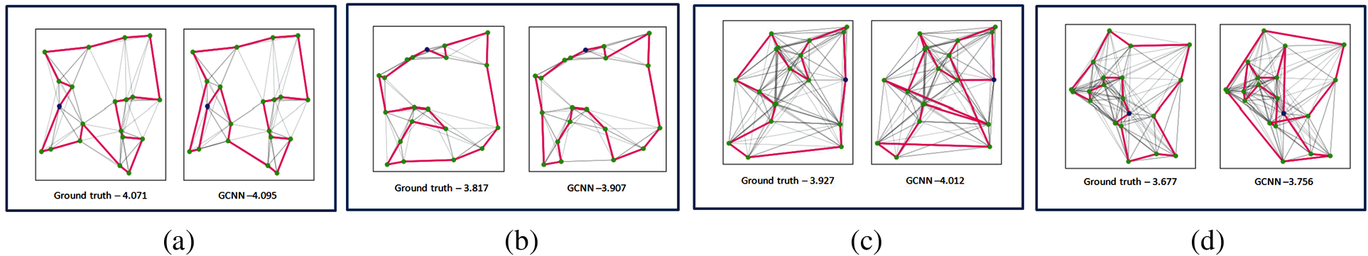
Figure 6: Sample Output - TSP20 model with its predicted tour length (a) and (b) Edges - 5, (c) and (d) Edges - 10
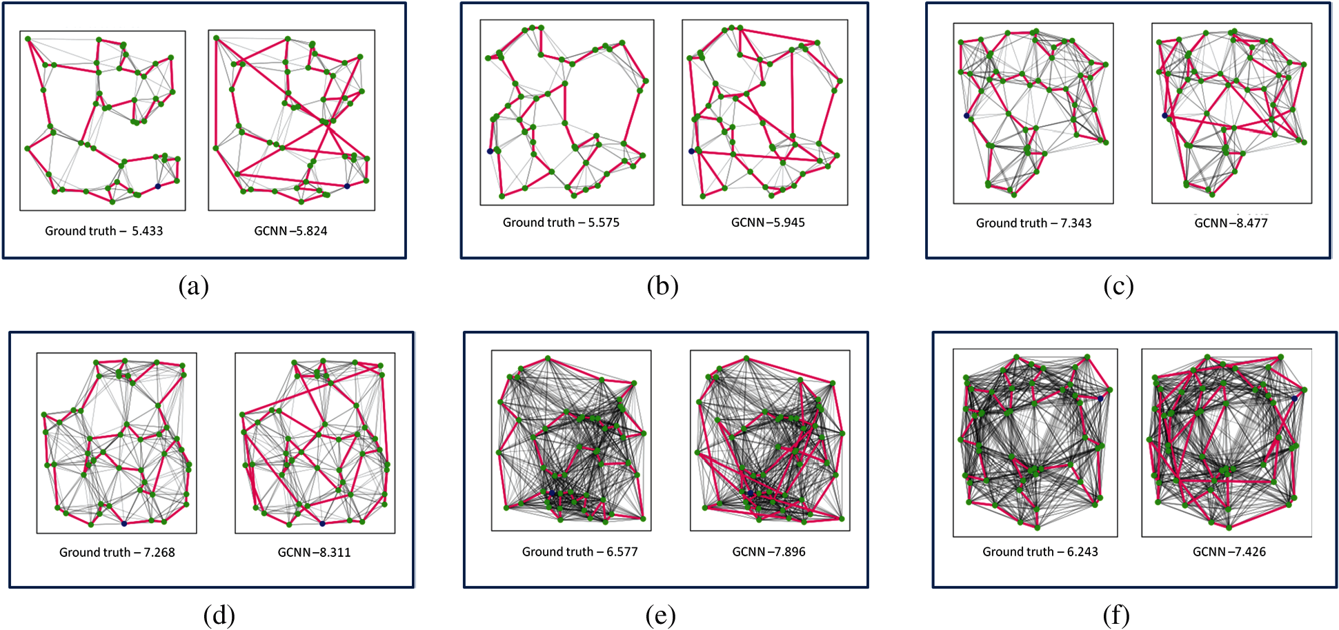
Figure 7: Sample output - TSP50 model with its predicted tour length a) and (b) Edges - 5, (c) and (d) Edges - 10, (e) and (f) Edges - 25
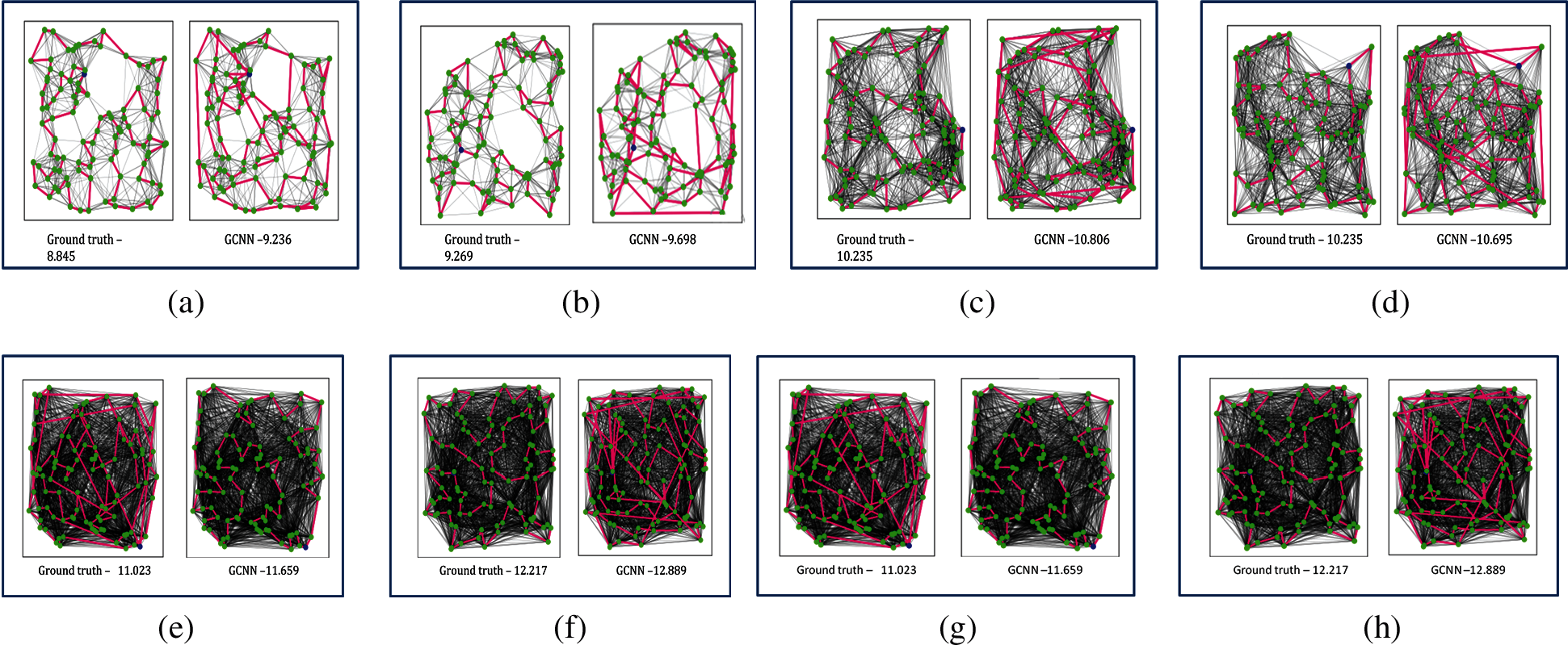
Figure 8: Sample output - TSP100 model with its predicted tour length (a) and (b) Edges - 5, (c) and (d) Edges - 10, (e) and (f) Edges - 25, (g) and (h) Edges -50
The model had a total of 30 layers with 3 multi-layer perceptrons. The total number of parameters used within the model was approximately about 11054402. Talking about the batch sizes used for the training purposes, the problem instances were divided into 20 batches while having 500 batches per epoch. The total time consumed for generating one single batch took approximately 0.144 sec. Tab. 1 shows the various model parameters used for building the network. It also discusses various results obtained while considering TSP20, TSP50, and TSP100 models, where 20, 50, and 100 are the number of nodes considered for the training purposes.

In each model, we have tested the predicted tour length of 5 graphs with various probabilities of the neighboring nodes. The optimal gap denotes the gap obtained between the values of the ground truth tour lengths to the values of the predicted tour lengths while considering the total time consumed for obtaining the optimal solution. It can be seen that the proposed approach can give approximately the near-optimal solution while considering graphs with lesser nodes when compared to the graphs with larger node sizes. The mean optimal gap is found for the tour obtained while considering the same number of neighbor nodes to get the optimality gap in the predicted tour lengths by GCN. The change in the optimality gap as tabulated in Tab. 1, while increasing the number of neighbor nodes in various models can be observed in Fig. 9. In Fig. 10, sample graphs G1, G2, G3, and G4 from the TSP20, 50, and 100 models are taken to illustrate the difference in the tour lengths.
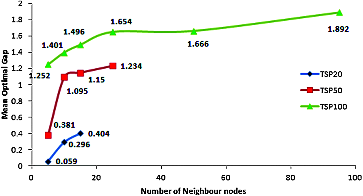
Figure 9: Optimality Gap obtained for various TSP models
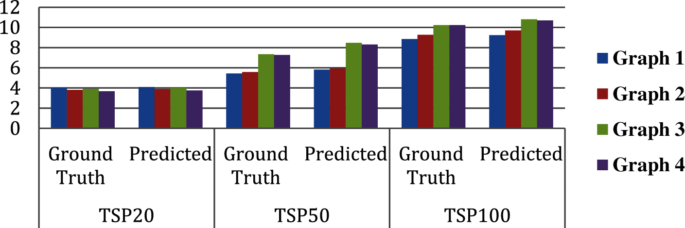
Figure 10: Sample output from TSP20, 50 and 100 models - Ground truth vs. Predicted path
After the evaluation is done by taking the graphs from the test data, the model is tested with self-constructed graphs. These graphs are the ones obtained by partitioning few study areas using the rectilinear partitioning algorithms as mentioned in [17]. Self-constructed graphs are obtained as shown in Fig. 11, whose points of coverage are the centroids of the partitions which are further considered to be the vertices for solving TSP. Firstly all the possible paths connecting the vertices are obtained to form the adjacency matrix using GCN. Then this is used by the heuristic search algorithm to find the optimal path. The optimal path is then compared with evolutionary algorithms such as ACO, PSO, and FA to evaluate the performance of the proposed methodology. A sample self-constructed graph is depicted in Fig. 12. where the optimal path is obtained using various techniques.
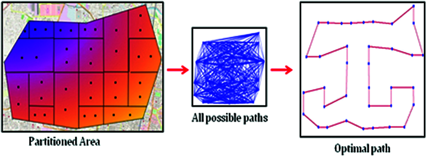
Figure 11: Optimal path obtained using Rectilinear Partitioning Algorithm
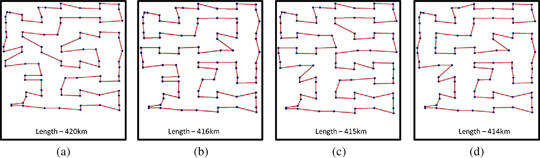
Figure 12: Visualization of graphs using various techniques (a) PSO (b) ACO (c) FA (d) GCN
Tabs. 2 and 3, show the comparison of the predicted tour length and overall execution time obtained for a set of 10 graphs using various techniques. It can be observed that the PSO gives a very high tour length when compared to other techniques in most cases while the Firefly algorithm giving the most optimal path. Tour prediction using our proposed work predicts an approximate optimal path in a lesser time when compared to other techniques. From Figs. 13a and 13b, it could be stated that the optimal tour for any given graph is obtained while making use of evolutionary algorithms but they consume a lot of time for the prediction as to the number of places to be visited increases. Whereas, to obtain the optimal tour in very minimal time it is better to make use of the proposed model using GCN as they seem to work well even while using larger graphs.


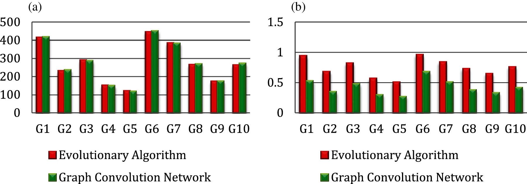
Figure 13: Evolutionary algorithm vs. graph convolution network (a) tour length (in kms) (b) execution time (in secs)
Efficient path planning of UAVs has become one of the most researched areas nowadays as most of the applications now rely on the deployment of UAVs without human intervention. The Coverage Path Planning(CPP) problem is one of the most important problems that need to be focused upon while deploying a UAV in any real-time surveillance application. This paper assumes that a geographic map is given and an optimal flying path for a UAV, covering the entire area is to be found out. The path of the UAV is to be designed in such a way that it starts at a point and visits each of the given points of coverage once and ends at the same point where it started. In this paper, a deep learning framework based on Graph Convolution Network is proposed for finding optimal tours for a given TSP instance. The network is initially trained using the Concorde Benchmark Dataset. The idea behind the usage of GCN is to reduce computation time compared to other techniques including evolutionary algorithms. The framework attempts to obtain an efficient solution with minimal training data. The performance of GCN is compared with that of the other evolutionary techniques. The performances of Particle Swarm Optimization, Ant Colony Optimization, and Firefly Algorithms on graphs of sizes up to 100 nodes, are used for this comparison. It could be concluded that the optimal tour for any given graph is obtained while making use of evolutionary algorithms but they consume a lot of time for the prediction as the number of points to be visited increases. Whereas, to obtain the optimal tour in very minimal time it is better to make use of the proposed model using GCN as they seem to work well even while using larger graphs. Future work could include the use of the Steiner tree for partitioning the area. Partitioning of the area could also involve dynamic obstacles into consideration as UAVs need to be deployed in real-time scenarios.
Funding Statement: The authors received no specific funding for this study.
Conflicts of Interest: The authors declare that they have no conflicts of interest to report regarding the present study.
1. I. U. Khan, I. M. Qureshi, M. A. Aziz, T. A. Cheema and S. B. H. Shah, “Smart IoT control-based nature inspired energy efficient routing protocol for flying ad hoc network (FANET),” IEEE Access, vol. 8, no. 1, pp. 56371–56378, 2020. [Google Scholar]
2. J. Akshya and P. L. K. Priyadarsini, “A hybrid machine learning approach for classifying aerial images of flood-hit areas,” in Proc. ICCIDS, Chennai, Tamil Nadu, India, pp. 1–5, 2019. [Google Scholar]
3. I. U. Khan, R. Alturki, H. J. Alyamani, M. A. Ikram, M. A. Aziz et al., “RSSI-controlled long-range communication in secured IoT-enabled unmanned aerial vehicles,” Mobile Information Systems, vol. 2021, no. 1, pp. 1–11, 2021. [Google Scholar]
4. S. Zhang, H. Tong, J. Xu and R. Maciejewski, “Graph convolutional networks: A comprehensive review,” Computational Social Networks, vol. 6, no. 1, pp. 626, 2019. [Google Scholar]
5. I. U. Khan, S. Z. Nain Zukhraf, A. Abdollahi, S. A. Imran, I. M. Qureshi et al., “Reinforce based optimization in wireless communication technologies and routing techniques using internet of flying vehicles,” in Int. Conf. on Future Networks and Distributed Systems, St.petersburg, Russia, pp. 1–6, 2020. [Google Scholar]
6. J. Akshya and P. L. K. Priyadarsini, “Graph-based path planning for intelligent UAVs in area coverage applications,” Journal of Intelligent & Fuzzy Systems, vol. 39, no. 6, pp. 8191–8203, 2020. [Google Scholar]
7. H. Azpúrua, G. M. Freitas, D. G. Macharet and M. F. Campos, “Multi-robot coverage path planning using hexagonal segmentation for geophysical surveys,” Robotica, vol. 36, no. 8, pp. 1144–1166, 2018. [Google Scholar]
8. W. P. Coutinho, R. Q. D. Nascimento, A. A. Pessoa and A. Subramanian, “A branch-and-bound algorithm for the close-enough traveling salesman problem,” INFORMS Journal on Computing, vol. 28, no. 4, pp. 752–765, 2016. [Google Scholar]
9. A. Sonmez, E. Kocyigit and E. Kugu, “Optimal path planning for UAVs using genetic algorithm,” in Proc. ICUAS, Denver, Colorado, USA, pp. 50–55, 2015. [Google Scholar]
10. T. S. Alemayehu and J. H. Kim, “Efficient nearest neighbor heuristic TSP algorithms for reducing data acquisition latency of UAV relay WSN,” Wireless Personal Communications, vol. 95, no. 3, pp. 3271–3285, 2017. [Google Scholar]
11. P. Merz and J. Huhse, “An iterated local search approach for finding provably good solutions for very large TSP instances,” in Proc, PPSN X. Dortmund, Germany, pp. 929–939, 2008. [Google Scholar]
12. D. Karapetyan and G. Gutin, “Lin-Kernighan heuristic adaptations for the generalized traveling salesman problem,” European Journal of Operational Research, vol. 208, no. 3, pp. 221–232, 2011. [Google Scholar]
13. L. Xin, W. Song, Z. Cao and J. Zhang, “Step-wise deep learning models for solving routing problems,” IEEE Transactions on Industrial Informatics, vol. 17, no. 7, pp. 4861– 4871, 2021. [Google Scholar]
14. H. Taguchi, X. Liu and T. Murata, “Graph convolutional networks for graphs containing missing features,” Future Generation Computer Systems, vol. 117, no. 5, pp. 155–168, 2021. [Google Scholar]
15. W. L. Chiang, X. Liu, S. Si, Y. Li, S. Bengi et al., “Cluster-gcn: An efficient algorithm for training deep and large graph convolutional networks,” in Proc. KDD’19, Anchorage AK, USA, pp. 257–266, 2019. [Google Scholar]
16. A. Nammouchi, H. Ghazzai and Y. Massoud, “A generative graph method to solve the Travelling Salesman Problem,” in Proc. MWSCAS, Springfield, MA, USA, pp. 89–92, 2020. [Google Scholar]
17. J. Akshya and P. L. K. Priyadarsini, “Area Partitioning by Intelligent UAVs for effective path planning using Evolutionary algorithms,” in Proc. ICCCI, Coimbatore, Tamil Nadu, India, pp. 1–6, 2021. [Google Scholar]
 | This work is licensed under a Creative Commons Attribution 4.0 International License, which permits unrestricted use, distribution, and reproduction in any medium, provided the original work is properly cited. |