Intelligent Automation & Soft Computing DOI:10.32604/iasc.2022.020551
Article

Quantum Firefly Secure Routing for Fog Based Wireless Sensor Networks

R. Dayana1,* and G. Maria Kalavathy2

1Department of Computer Science and Engineering, Jeppiaar Institute of Technology, Chennai, 631604, Tamil Nadu, India
2Department of Computer Science and Engineering, St. Joseph’s College of Engineering, Chennai, 600119, Tamil Nadu, India
*Corresponding Author: R. Dayana. Email: dayanacse006@gmail.com
Received: 29 May 2021; Accepted: 20 July 2021

Abstract: Wireless Sensor Networks (WSNs) become an integral part of Internet of Things (IoT) and finds their applicability in several domains. As classical WSN faces several issues in service-based IoT applications, fog computing has been introduced in real-time, enabling local data processing and avoid raw data transmission to cloud servers. The Fog-based WSN generally involves advanced nodes, normal nodes, and some Fog Nodes (FN). Though the Fog-based WSN offers several benefits, there is a need to develop an effective trust-based secure routing protocol for data transmission among Cluster Heads (CHs) and FNs. In this view, this paper presents a Quantum Firefly Optimization based Multi-Objective Secure Routing (QFO-MOSR) protocol for Fog-based WSN. The main intention of the QFO-MOSR technique is to derive an optimal selection of routes between CHs and FNs in the network. The QFO-MOSR technique has incorporated the concepts of quantum computing and Firefly (FF) optimization algorithm inspired by the flashing behaviour of FFs. In addition, a multi-objective fitness function is derived by the QFO-MOSR technique using seven objectives: distance, inter-cluster distance, energy, delay, intra-cluster distance, link lifetime, and trust. The proposed routing technique derives a fitness function including trust factor from ensuring security. The design of the QFO-MOSR technique with a multi-objective fitness function shows the novelty of the work. To validate the performance of the QFO-MOSR technique, a series of experiments were carried out, and the results are investigated in terms of different measures. The experimental analysis ensured that the QFO-MOSR technique is superior to other methods in terms of different measures.

Keywords: Fog computing; internet of things; wireless sensor networks; energy efficiency; cluster heads; firefly algorithm; fitness function

1  Introduction

Next-generation Wireless Sensor Networks are expected to be placed in Internet of Things (IoT). The IoT has transformed the present world of technology. The electronic devices such as home appliances, medical equipment, cameras etc., can interact via the internet connecting several Sensor Nodes (SN). Therefore, these devices have few restrictions and involve processing power, bandwidth, storage, and a restricted power source. WSN is widely utilized in the monitoring activities of the present society like heat energy in greenhouses, emission from hydraulic power plants, forest fire, and production of vehicles in the automobile industry.

In traditional WSN, the SN can transfer their raw data to BS for storage and analysis. Current developments in IoT technology have allowed WSN for transferring raw data to the cloud for storage and processing [1,2]. But rather than transferring the large quantity of sensed data produced in the SN on the network and later process them by utilizing a Cloud Computing (CC) framework, a few processes are executed nearer to the WSN using fog computing. Fog computing consists of network devices like proxy servers, routers, gateways, and set-top boxes [3]. These devices have high processing ability and memory compared to other SN. This method does not preserve SN’s energy dissipation in communication; however, it offers location awareness, higher bandwidth, and lower latency for WSN. Cisco’s ‘Fog Computing’ was established to conquer restrictions in CC [4,5]. They contain a power source, higher processing power, and more storage for fog servers from the network. This novel technique is designed at the end of the network. It provides various advantages for end-users and involves fewer bottlenecks, data security, effective network bandwidth utilization, high speed of analysis resolving higher latency over the network, and increased trustworthiness of transmitted sensed data.

The combination of fog computing with WSN and IoT makes a novel kind of service named Fog as a Service (FaaS). But for the absolute utilization of fog computing, every fog node should satisfy the following conditions: (i) simultaneous data collection from lower end nodes, (ii) high processing power and efficiency for supporting real-world data analysis and processing, (iii) higher service trustworthiness, and (iv) low power utilization, to attain long time exploitation. In the WSN framework, they offer to the elemental SN. The combination of fog computing with WSN could conquer several challenges. In hierarchical WSN, a sink node, i.e., a CH, is generally utilized for aggregating the sensed data in cluster members, and cluster routing protocols are placed to decrease the energy consumption and network traffic [6]. Thus, the balanced load of hierarchical WSN is a significant problem that defines an entire network’s efficiency. Simultaneously, at a higher level, CH is compromised and captured, which would influence the data security of the whole network [7,8]. Generally, these security attacks are classified as internal and external attacks for WSN.

This paper presents a Quantum Firefly Optimization based Multi-Objective Secure Routing (QFO-MOSR) protocol for Fog-based WSN. The QFO-MOSR technique is derived from the concepts of quantum computing and the FF optimization algorithm. Besides, a multi-objective fitness function is derived by the QFO-MOSR technique using seven objectives: distance, inter and intra-cluster distance, energy, delay, link lifetime, and trust. The design of the QFO-MOSR technique with a multi-objective fitness function shows the novelty of the work. To validate the performance, the QFO-MOSR, including the trust factor in the fitness function, ensures security. To investigate the effectual outcome of the QFO-MOSR technique, simulations occur, and the results are examined under distinct dimensions. In short, the contributions of the paper are listed as follows.

•   Design a new QFO-MOSR technique for Fog-based WSN.

•   Design a fitness function using seven inter-related parameters to select CH.

•   Include trust factor in the fitness function to ensure security in Fog-based WSN.

•   Validate the performance of the QFO-MOSR technique using the Network Simulator (NS)-3.

2  Literature Review

Fang et al. [9] presented a Gaussian Distribution based Comprehensive Trust Management System (GDTMS) for FIWSN. Additionally, their trust decision, namely, the grey problem solving, is presented to attain the tradeoff between security energy consumption and transmission efficiency. The presented tradeoff could efficiently choose the secure and robust transmit node, specifically the trust management-based secure routing system. Additionally, the proposed method is also appropriate to defend against bad-mouthing attacks. Arapoglu et al. [10] proposed a GDTMS for FIWSN. Moreover, in this trust management, the analytical hierarchy procedure is presented to attain the tradeoff between energy consumption security and transmission efficiency. The presented trade-off could efficiently choose the robust and secure transmit node. In Fang et al. [11], a Lightweight Trust Management Scheme (LTMS) is presented depending upon binomial distribution for protecting from internal attacks. Concurrently, environment, energy, distance, and security domains are assumed and presented to a Multi-dimensional Secure Clustered Routing (MSCR) system by utilizing dynamic dimensional weight in hierarchical WSN. Revanesh et al. [12] proposed a distributed protocol named Secure Coronas Based Zone Clustering and Routing (SC-ZCR). Abidoye et al. [13] proposed an effective routing protocol for data transmission in WSN known as energy effective hierarchical routing protocol for WSN based on fog computing. Fog computing is combined with the presented system because of its ability to enhance the restricted power source of WSN and the need for IoT applications. Furthermore, they proposed an enhanced ACO method to construct an optimum path for effective data transmission to SN. Cara et al. [14] developed and designed a wireless SN for fog computing architecture to address two significant problems: deployment and development of strong transmission facilities, such as network resilience provisioning and energy consumption. The implementation is directed by investigating the related macro architectural feature and functioning limitations of the network architecture. Wang et al. [15] presented a Fog-based hierarchical trust method for this cybersecurity deficiency. This hierarchical method comprises two divisions, trust among Cloud Service Providers (CSP) and trust in the basic framework and Sensor Service Provider (SSP). Rafi et al. [16] presented an enhanced LEACH protocol called LEACH with Dijkstra’s Algorithm (LEACH-DA) in a cloud platform that enhances the power utilization/energy use depending upon shorter path selection. Similarly, the presented architecture includes load balance by selecting a suitable CH node between its alternative by estimating its traffic condition with the base station or cloud. Moreover, they utilize a fog computing module for this condition (i.e., LEACH-DA-Fog) to raise the network lifetime related to the actual execution of the basic protocol. Borujeni et al. [17] presented a novel technique depending upon Fog-based energy-efficient routing protocol for WSNs (P-SEP) that utilizes ACO-based routing of FN (FEAR) and PEGASIS-based routing of FN (FECR) methods in execution. This method develops the efficiency of fog enabled WSN and extends the network lifespan. The efficiency of the presented technique is calculated towards P-SEP. Though several techniques are available in the literature, there is still a need to design a new protocol to achieve energy efficiency and security in Fog-based WSN. Besides, most of the works have not considered the interrelated metrics and trust factors to select CHs.

3  The Proposed QFO-MOSR Model

Fig. 1 showcases the overall working process of the QFO-MOSR model. The proposed QFO-MOSR model aims to select the routes to the destination optimally. Once the presented model derives a fitness function, the possible paths towards the destination are identified. Followed by that, the QFO-MOSR model chooses an optimal route to the destination from the available paths. A significant component in introducing the technique is solution encoding. The proposed technique for detecting an optimum path from source (S) to destination (D) is assumed as a binary search problem. Here, D = {p_1, p_2, … , p_k} denotes destination containing ‘k’ paths created using an intermediate node among S and D nodes [18]. The number in the network is based on node count N, thus the interval 0 ≤ p_k ≤ N. Henceforth, the solution count present in the network among S and D is denoted by S ^ E = {1, 2, …, k}, in which ‘k’ indicates the overall number of paths. The k solution count is present among S and D pairs. This technique detects an optimal path with maximal trust, and another chosen objective utilizes multi-objective FF, which is determined by the following sections.

3.1 Design of QFO Algorithm

FF is a moderately novel technique that is established in [19]. This method is based on specific behavioural patterns, mainly flashing features of fireflies in the tropical summer sky. Fireflies belong to the insect family known as Lampyridae. Firefly is a type of beetle, which uses the concept of bioluminescence for attracting prey/mates. The luminance made by FF allows other fireflies to trail their path after prey.

Few flashing features of fireflies have been idealized to improve the FF method. Every FF is considered unisex to an individual FF that would attract another FF.

1.    The attraction of an individual FF to other is relative to its intensity, by increasing the distance among them; subsequently, the one with lesser intensity would often move towards high brightness. When there is no brighter FF than a provided FF, it will move arbitrarily.

2.    The brightness/light intensity of FF is defined using the landscape of objective function to be improved.

Figure 1: Working process of QFO-MOSR model

The light intensity of one FF is caused by the nature of the encoded cost function, and the intensity is about the value of FF. The main problem in FF growth is the creation of objective function (i.e., attractiveness) and difference in the light intensity. Hence, reduction of light intensity is because of distance among fireflies that results in differences of intensity and thus, reduce the attraction between them. Eq. (1) is utilized for representing light intensity with changing distance:

I(r)=I0exp(−γ⋅r2), (1)

where I represents brightness of S at D r from firefly, I0 denotes early light intensity if r=0 ; and C indicates light absorption coefficient that describes the difference of attraction and impacts the cFF algorithm’s convergences speed and entire performance [20]. C usually differs from 0.1 to 10. Since FF attraction is related to brightness witnessed by nearby FFs, they could denote attraction β at Cartesian distance r from FF, which is given by Eq. (2):

β=β0exp(−γ⋅r2), (2)

where β0 represents attraction at a distance r=0. The light intensity I and attraction β are similar manners. The distance among two FFs i and j at xi and xj is given by Eq. (3):

rij=||xi−xj||. (3)

The motion of FF i attracted by another brighter FF ‘ j ’ is given as:

Δxi=β0e−γ⋅rij2(xjt−xit)+α(Nrand−0.5), (4)

where t represents iteration. The initial term is performed in Eq. (4) due to attractiveness. Another term α(Nrand−0.5) denotes randomization and increases the search space. α indicates the randomization coefficient and arbitrary amount vector acquired from Gaussian Distribution α∈[0 , 1 ] . The value Nrand denotes in ‘0’ and ‘1’. The succeeding motion of FF i is upgraded by Eq. (5):

xit+1=xit+Δxi. (5)

The motion of FFs includes; the present location of i th FF, attracted to other fireflies, and arbitrary walk containing randomization variable α and arbitrarily created number from the range ‘0’ and ‘1’. Where β0=0 , the motion is based on the arbitrary walk. In contrast, variable C contains a critical effect on convergence speed. Besides the initial step, each performance is continually executed till the optimization procedure is terminated.

For improving the effectiveness of the FF algorithm, the QC concept is integrated into it. QC is current research on quantum computers by occurrences of quantum methods like the quantum gate, state superposition, and entanglement [21]. The primary data unit in QC is the Q bit. It might be in state |0>, |1> or superposition of states |0> and |1> concurrently. With Dirac notation, the Q bit denoted by the integration of states |0> and |1> is given as Eq. (6):

|Q>=α|0+β|1⟩suchthat|α|2+|β|2=1 (6)

where α and β represent complex numbers. |α|2 (resp. |β|2 ) denotes likelihood for finding Q -bit in state zero (denoted in state one). A quantum register of size n is later established from a group of nQ bits. It denotes as the superposition of nQ bits, and mainly it comprises till 2n probable values concurrently. A quantum register is as follows Eq. (7):

Ψ=∑x=02n−1⁡CX|X⟩ (7)

The amplitude Cx fulfils the succeeding Eq. (8):

∑x=02n−1⁡|CX|2=1 (8)

The Q bit state is altered using a Quantum gate ( Q gate) [22]. A Q gate is a reversible gate denoted by unitary operator U act on Q bit basis state fulfilling U+U=UU+ , in which U+ indicates Hermitian adjoint of U . There are several Q gates, like the controlled-NOT, Hadamard, Rotation, NOT gate, and so on. Fig. 2 demonstrates the QFO technique’s flowchart. They utilize rotation angle in Q bit depiction, whereas every quantum FF solution Qfi ( i th quantum FF in a quantum population) relates to vector Θi=(θi1,…,θim) of parameters θij with θij∈[0,π2] for (1≤j≤m) .

Every quantum FF solution Qfi represents a string of quantum bits, evaluated by: Eq. (9)

Qfi=[cos(θi1)|cos(θi2)|⋯|cos(θim)sin(θi1)|sin(θi2)|⋯|sin(θim)] (9)

The likelihood amplitude of a single quantum bit is determined by a pair of amounts ( cos(θij),sin(θij) ) in which |cos(θij)|2 denotes the likelihood of eliminating item xj and |sin(θij)|2 that embodies the likelihood of choosing the item xj ( i th binary firefly). cos(θij) and sin(θij) fulfil Eq. (10):

|cos(θij)|2+|sin(θij)|2=1. (10)

Figure 2: Flowchart of QFO

Firefly Algorithm

Need: β0 , γ

Generate an early population of n fireflies with d dimension search:

xik , i=1,…,n and k=1,…,d ;

Calculate the population fitness (f(xi) , which is equivalent to the brightness Ii );

while (not end criteria) Do

For ( i=1 : n : every firefly) Do

For ( j=1 : n : each firefly) Do

If (Ii<Ij) Then

Move FF ‘ i ’ towards ‘j′ in d dimensional;

End If

Attraction differs with distance ‘r′ by exp[−r2] ;

Calculate novel solutions and upgrade brightness;

End For

End For

End While

Ranking the FFs and detect an optimum solution

End If

End

Firefly Algorithm

Need: β0 , γ

Generate an early population of n fireflies with d dimension search:

xik , i=1,…,n and k=1,…,d ;

Calculate the population fitness (f(xi) , which is equivalent to the brightness Ii );

while (not end criteria) Do

For (i=1 : n : every firefly) Do

For (j=1 : n : each firefly) Do

If (Ii<Ij) Then

Move FF ‘i ’ towards ‘j′ in d dimensional;

End If

Attraction differs with distance ‘r′ by exp[−r2] ;

Calculate novel solutions and upgrade brightness;

End For

End For

End While

Ranking the FFs and detect an optimum solution

End If

End

3.2 Application of QFO Algorithm for Secured Routing Process

The FF is calculated to find an optimum solution from the collection of variables. The fitness calculated for the presented QFO-MSR model utilizes 7 variables, such as link lifetime, delay, distance, energy, intra-cluster distances, trust model, and inter-cluster distances are utilized for routing. Now, the fitness is assumed by maximization operation. Henceforth, the solution offering maximal value of fitness is assumed to multi-hop routing. It is Eq. (11) as,

O=W1×P+W2×(1−T)+W3×(1−X∗)+W4×X+W5×(1−D)+W6×M+W7×N (11)

where W1,W2,W3,W4 , W5 , W6 , and W7 denotes weight calculated by fuzzy membership operation. P denotes node energy, T indicates transmission delay, X∗ represents inter-cluster distance, D indicates distance among two hops, X denotes intra-cluster distance and M indicates link time, and the trust module is represented by N . Eq. (12) calculates the weight,

W={0;if r<fr−fp−f;if f≤r≤pq−rq−p;if p≤r≤q0;if r≥q (12)

where p , q , and r denotes vertices of triangular membership function T(f) . Now, p indicates low boundary, q represents medium boundary with membership value one, and r denotes upper boundary with membership value ‘0’ [23].

i) Energy: The network energy is determined by the energy summation of each hop that denotes energy continued in nodes. The energy contains higher value, and it is Eq. (13) as:

P=1b∑n=1b⁡E(Jn) (13)

where b denotes hop count, which cooperates in multi-hop routing and E(Jn) denotes energy of nth hop.

ii) Delay: The delay is calculated by hop, which plays in routing and the delay have to be lesser to perform effectual routing. The delay calculated by the ratio of hop essential for routing overall nodes limited in WSN is Eq. (14) as:

T=bl (14)

where l denotes overall nodes existing in WSN, and b represents the overall hop count required for routing.

iii) Intra-cluster Distance: It can be estimated using the summation of distance among hops, and the separate node existing in the hop is minimum. When it is minimal, the node is nearer to the hop; thus, the energy and data loss decrease. It is Eq. (15) as:

X=1b(∑n=1b⁡∑t∈ks⁡X(Jn,Lt)β) (15)

where, β denotes regularization factor, X(Jn,Lt) denotes distance among nth hop and tth node and the overall nodes are denoted by s.

iv) Inter-cluster Distance: The ratio of distance calculated among 2 clusters is the so-called inter-cluster distance, and it has to be maximum to provide an efficient routing. It is Eq. (16) as follows,

X∗=(∑x=1no⁡∑t=x+1no⁡X(Gx,Gt)β) (16)

where X(Gx,Gt) denotes distance among two clusters, and no denotes overall CHs.

v) Distance: The summation of distance calculated amongst two hops is given by Eq. (17). The distance has to be maximum to multi-hop routing as follows,

D=1b×(∑n=1b−1⁡X(Jn,Jn+1)β) (17)

vi) Link Lifetime: The network lifetime is acquired from the link lifetime and must be maximum for attaining an efficient routing. It is given in Eq. (18).

M=1b×∑n=1b−1M(Jn,Jn+1)β (18)

where, M(Jn,Jn+1) denotes link lifetime of nth and (n+1)th hops.

vii) Trust model: It gives security to the proposed method in the routing procedure. It is utilized for calculating the trust of agents with suspicious behaviour. Numerous variables are assumed for calculating the trust that includes integrity and forwarding rate factors, direct and indirect trusts. Now, every hop in WSN gives a high trust degree to evaluate the trust level among hops and adjacent hops. It is Eq. (19) as:

N={Nd+Ni+NF+NI} (19)

where, Nd denotes direct trust, Ni indicates indirect trust, NF denotes forwarding rate factor, and NI represents integrity factor.

viii) Direct Trust: It is called local trust, and it presents the trust value of agent computed from familiarity while communicating with targeted agents Eq. (20).

(Nd)yz(n,n+1)=funyz(n,n+1) (20)

where, (Nd)yz denotes direct trust for yth transaction and zth the time interval, fun denotes satisfaction measure, y represents transaction, z indicates time interval, n denotes calculation hop, and n+1 indicates hop to be calculated. The fulfilment measures are utilized for computing fulfilment degrees of an agent, which contain stated service. Therefore, the fulfilment measures keep the record of fulfilment level using exponential average upgrade functions as follows Eq. (21),

funyz(n,n+1)=η×funv+(1−η)×funy−1z(n,n+1) (21)

where, funv denotes fulfilment value of the current transaction, and funy−1z(n,n+1) denotes fulfilment value of y−1 transaction at zth time interval, η represents weight Eq. (22).

funv={0;iftransactionisthoroughlyunsatisfactory1;ifthetransactionisfullysatisfactory∈(0,1);otherwise (22)

The weight g differs according to accumulated deviations Zyz(n,n+1) as follows

η=Y+j×γyz(n,n+1)1+Zyz(n,n+1) (23)

γyz(n,n+1)=|funy−1z(n,n+1)−funv| (24)

Zyz(n,n+1)=j×γyz(n,n+1)+(1−j)×Zy−1z(n,n+1) (25)

where Y denotes threshold and pose set value fixed to 0.25, j represents user-defined constant factor, γyz(n,n+1) indicates a current error, and Zyz(n,n+1) denotes accumulated deviations. Initially, the weight g is fixed to one, and it alters based on Eqs. (23)–(25)

ix) Indirect Trust: It is evaluated from knowledge attained using other hops. All hops use the knowledge of other hops for providing effective decisions to all transactions. For attaining this approach, each hop requests other hops for offering suggestions regarding other hops. The resulting hop gathers the recommendations from another hop together with feedback credibility of the suggested hop. Therefore, the indirect trust of nth hop regarding (n+1)th hop is as follows Eq. (26),

(Ki)yz(n,n+1)={∑a∈V−{n}⁡Hyz(n,a)×(Nd)yz(a,n+1)∑a∈V−{n}⁡Hyz(n,a);if|V−{n}|=00;If|v−{n}|>0 (26)

where, V denotes the collection of agents communicated with n+1 , a denotes hop that communicates with other hops to make forecast regarding marinating trust, feedback creditability is represented by Hyz The feedback credibility is used to compute the accurateness of feedback data which suggests hop given to the evaluator. Therefore, it is Eq. (27) by,

Hyz(n,n+1)={1−ln⁡(Syz(n,n+1))lnφifSyz(n,n+1)>φ0;otherwise (27)

where, Syz denotes similarity. The similarity measures are defined by determining that the two hops are equivalent. The comparison is calculated via detecting the customized variance depending upon fulfilment rating regarding the communicated agent and later uses the variance rating to describe comparison. Consequently, the comparison of two hops n and (n+1) is as follows Eq. (28),

Syz(n,n+1)={Sy−1z(n,n+1)+1−Sy−1z(n,n+1)ω;ifRyz(n,n+1)<lSy−1z(n,n+1)+Sy−1z(n,n+1)δ;otherwise (28)

where l denotes comparison deviation constant, E denotes collection of agents, x and d denote reward and punishment factors, and Ryz(n,n+1) denotes customized variance as follows Eq. (29),

Ryz(n,n+1)=∑a∈E(n,n+1)⁡(funyz(n,a)−funyz(n+1,a))|E(n,n+1)|2 (29)

x) Forwarding Rate Factor: The nodes in WSN have lesser energy distribution while transferring and sensing the information. Therefore, the collection of information finds out the possibility for examining and judging whether the node is assailed or not. Therefore, it is equated as follows Eq. (30),

(NF)z(n,n+1)=Az(n,n+1)Bz(n,n+1) (30)

where, Az(n,n+1) denotes the number of feedback packets, Bz(n,n+1) denotes the number of packets to forward, n indicates calculation hop, and n+1 represents hop to be estimated.

xi) Integrity Factor: If the data packet is relocated to an adjacent node, the S node studies whether the data packet interferes or not and finds whether the data packet is relocated in a particular time and guarantees reliability and accuracy of the data packet information. It is given by Eq. (31),

KI(n,n+1)=Uz(n,n+1)Ez(n,n+1) (31)

where, Uz(n,n+1) denotes the amount of wholly forwarded packets and Ez(n,n+1) denotes the number of packets to forward.

4  Performance Validation

This section examines the routing performance of the QFO-MOSR technique concerning different measures. The proposed model is simulated using a PC i5-8600k processor, GeForce 1050Ti, 4 GB RAM, 16 GB OS Storage, and 250 GB SSD File Storage. The simulation tool is used in NS3. Besides, the results are simulated in different measures under a varying number of rounds and nodes. A detailed comparative study of the QFO-MOSR technique with existing techniques also takes place. Tab. 1 and Fig. 3 investigate the QFO-MOSR technique’s lifetime analysis in terms of the Number of Alive Nodes (NAN). From the results, it can be clear that the QFO-MOSR technique has achieved improved outcomes with the higher NAN, whereas the FEAR technique has obtained the minor outcome with the lower NAN. For instance, under 500 rounds, the QFO-MOSR technique has attained an increased NAN of 492 rounds, whereas the FEAR, P-SEP, A Quantum Ant Colony Multi-Objective Routing (QACMOR), and Artificial Fish-Swarm (AFA) models have accomplished decreased NAN of 229, 488, 392, and 342 rounds, respectively. Then, under 1000 rounds, the QFO-MOSR approach has obtained an increased NAN of 395 rounds, whereas the FEAR, P-SEP, QACMOR, and AFA models have accomplished decreased NAN of 0, 225, 100, and 90 rounds correspondingly.

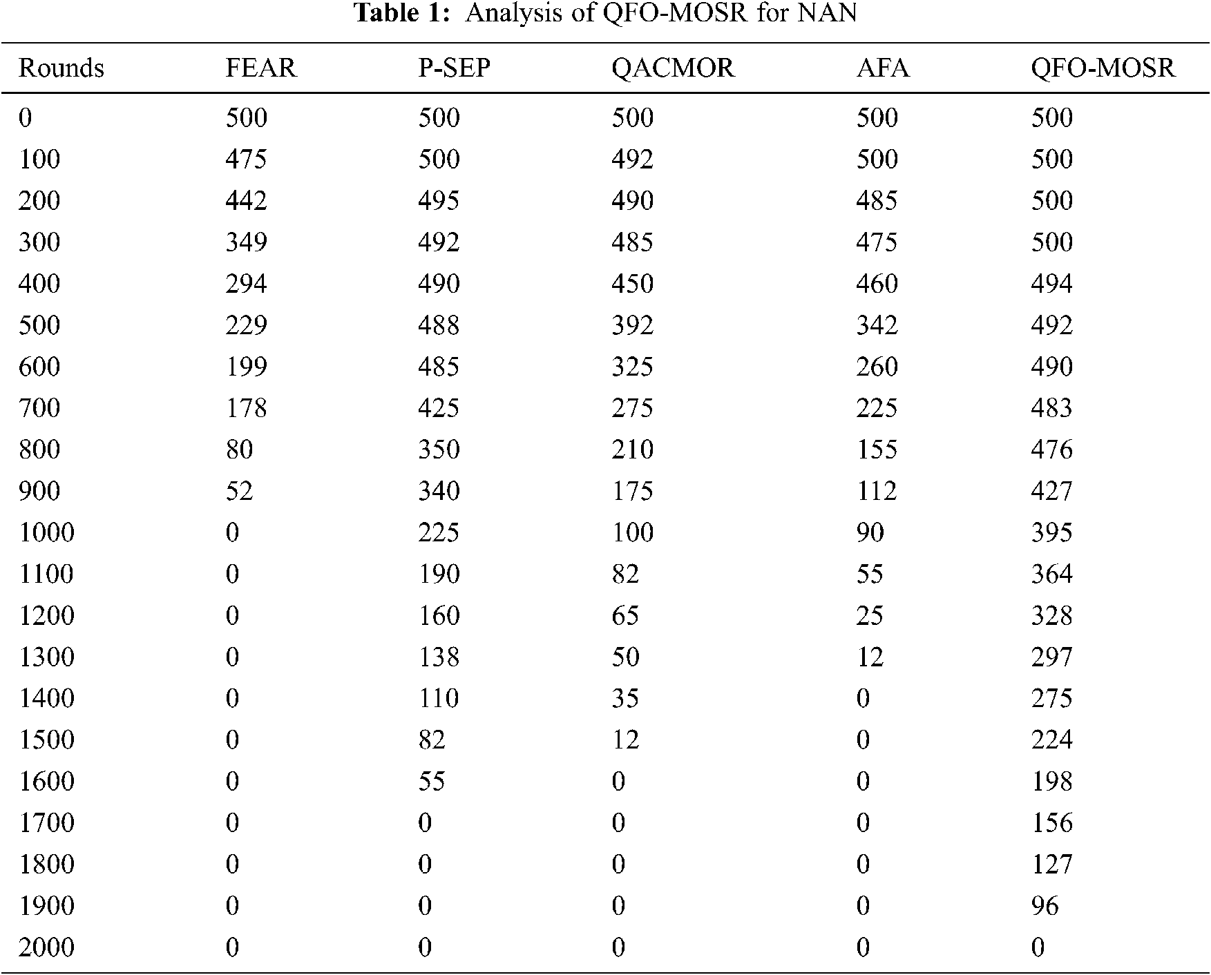
Figure 3: NAV analysis of QFO-MOSR

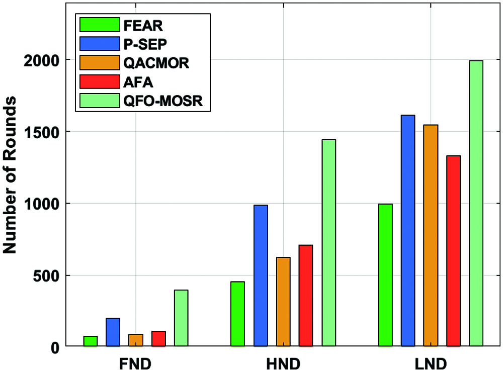
Figure 4: Analysis of QFO-MOSR

Likewise, under 1500 rounds, the QFO-MOSR technique has attained an increased NAN of 224 rounds, whereas the FEAR, P-SEP, QACMOR, and AFA techniques have accomplished decreased NAN of 0, 82, 12, and 0 rounds, respectively. Finally, under 1900 rounds, the QFO-MOSR technique has attained an increased NAN of 96 rounds, whereas the FEAR, P-SEP, QACMOR, and AFA models have accomplished decreased NAN of 0, 0, 0, and 0 rounds correspondingly. Comprehensive lifetime analysis of the QFO-MOSR technique takes place in Tab. 2 and Fig. 4. From the resultant values, it is apparent that the QFO-MOSR technique has depicted improved network lifetime. For instance, the QFO-MOSR technique has offered an FND of 397 rounds, whereas the FEAR, P-SEP, QACMOR, and AFA models have depicted a reduced FND of 75, 198, 88, and 111 rounds respectively.

Moreover, the QFO-MOSR model has offered an HND of 1442 rounds, whereas the FEAR, P-SEP, QACMOR, and AFA techniques have depicted a reduced HND of 445, 984, 625, and 711 rounds correspondingly. Furthermore, the QFO-MOSR technique has offered an LND of 1994 rounds, whereas the FEAR, P-SEP, QACMOR, and AFA methods have showcased a reduced LND of 995, 1612, 1544, and 1329 rounds correspondingly. A brief Average Residual Energy (ARE) analysis of the QFO-MOSR technique with existing methods is provided in Tab. 3 and Fig. 5. For instance, under 500 rounds, the QFO-MOSR approach has obtained a superior ARE of 0.494 J, whereas the FEAR, P-SEP, QACMOR, and AFA models have exhibited lower ARE 0.277, 0.4875, 0.3925, and 0.3425 J correspondingly. In addition, under 1000 rounds, the QFO-MOSR methodology has attained a maximum ARE of 0.406 J, whereas the FEAR, P-SEP, QACMOR, and AFA models have exhibited lower ARE of 0, 0.225, 0.1, and 0.09 J correspondingly. Also, under 1500 rounds, the QFO-MOSR technique has obtained a superior ARE of 0.218 J, whereas the FEAR, P-SEP, QACMOR, and AFA models have exhibited lower ARE of 0, 0.0825, 0.0125 and 0 J correspondingly. Additionally, under 1900 rounds, the QFO-MOSR algorithm has obtained a superior ARE of 0.054 J, whereas the FEAR, P-SEP, QACMOR, and AFA models have demonstrated minimum ARE of 0, 0, 0 and 0 J correspondingly.

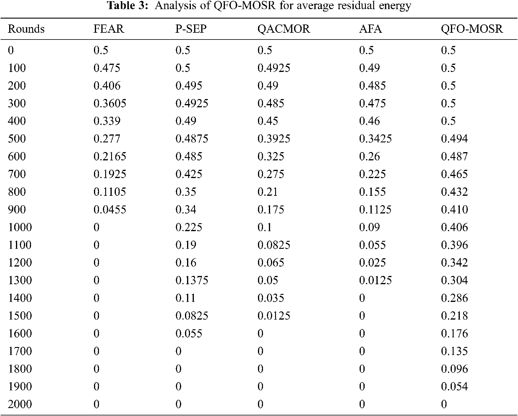
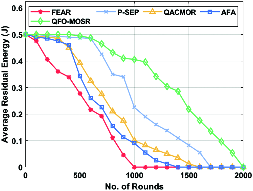
Figure 5: Average residual energy analysis of QFO-MOSR

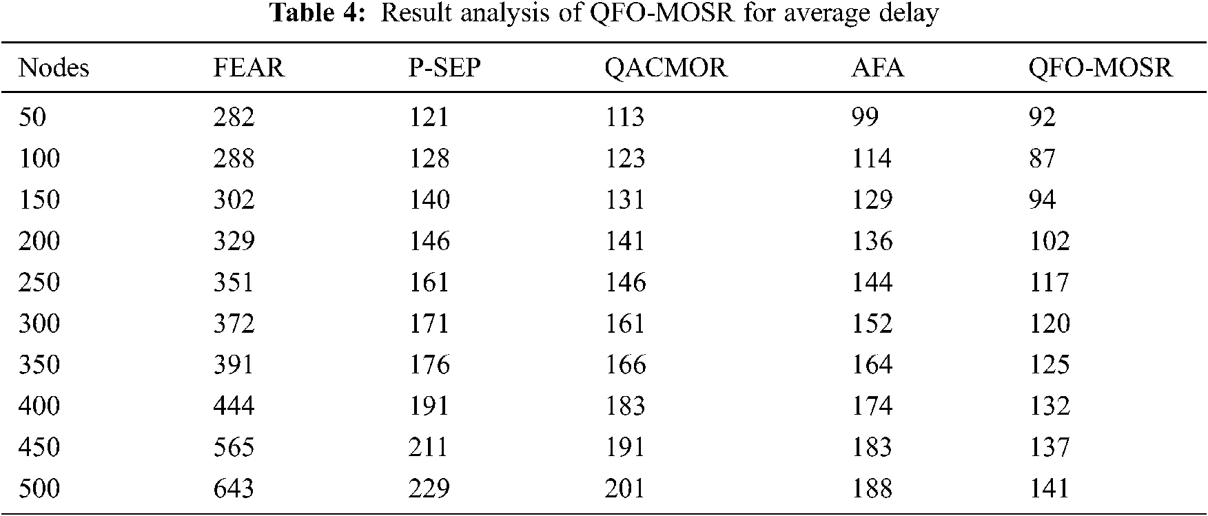
Brief average delay analysis of the QFO-MOSR method with existing techniques is provided in Tab. 4 and Fig. 6. For instance, under 50 nodes, the QFO-MOSR approach has attained a lesser average delay of 92 ms, whereas the FEAR, P-SEP, QACMOR, and AFA models have exhibited higher average delay 282, 121, 113 and 99 ms correspondingly. Besides, under 150 nodes, the QFO-MOSR approach has achieved a lesser average delay of 94 ms, whereas the FEAR, P-SEP, QACMOR, and AFA models have portrayed higher average delay of 302, 140, 131 and 129 ms, respectively. Moreover, under 300 nodes, the QFO-MOSR algorithm has attained a minimum average delay of 120 ms, whereas the FEAR, P-SEP, QACMOR, and AFA models have exhibited higher average delay of 372, 171, 161 and 152 ms, respectively. Furthermore, under 500 nodes, the QFO-MOSR model has achieved a minimum average delay of 141 ms, whereas the FEAR, P-SEP, QACMOR, and AFA models have exhibited maximal average delay 643, 229, 201 and 188 ms correspondingly.

A brief PDR analysis of the QFO-MOSR approach with existing techniques is provided in Tab. 5 and Fig. 7. For instance, under 50 nodes, the QFO-MOSR algorithm has achieved a superior PDR of 0.865%, whereas the FEAR, P-SEP, QACMOR, and AFA models have exhibited reduced PDR of 0.777%, 0.677%, 0.731%, and 0.747% correspondingly. In the meantime, under 200 nodes, the QFO-MOSR technique has reached a higher PDR of 0.841%, whereas the FEAR, P-SEP, QACMOR, and AFA models have exhibited minimal PDR of 0.727%, 0.607%, 0.677%, and 0.677% correspondingly. At the same time, under 350 nodes, the QFO-MOSR methodology has reached a higher PDR of 0.809%, whereas the FEAR, P-SEP, QACMOR, and AFA models have demonstrated lesser PDR of 0.697%, 0.537%, 0.607%, and 0.627% correspondingly. Meanwhile, under 500 nodes, the QFO-MOSR technique has reached a maximum PDR of 0.747%, whereas the FEAR, P-SEP, QACMOR, and AFA models have showcased minimal PDR 0.657%, 0.512%, 0.527%, and 0.567% correspondingly. A brief packet loss analysis of the QFO-MOSR approach with existing techniques is provided in Tab. 5 and Fig. 8. The figure has shown that the QFO-MOSR technique has showcased better results with minimal packet loss under the specific number of nodes. For instance, under 50 nodes, the QFO-MOSR approach has obtained a minimum packet loss of 0.0198, whereas the FEAR, P-SEP, QACMOR, and AFA methods have showcased higher packet loss of 0.2, 0.11, 0.07, and 0.04 correspondingly.

Figure 6: Average delay analysis of QFO-MOSR

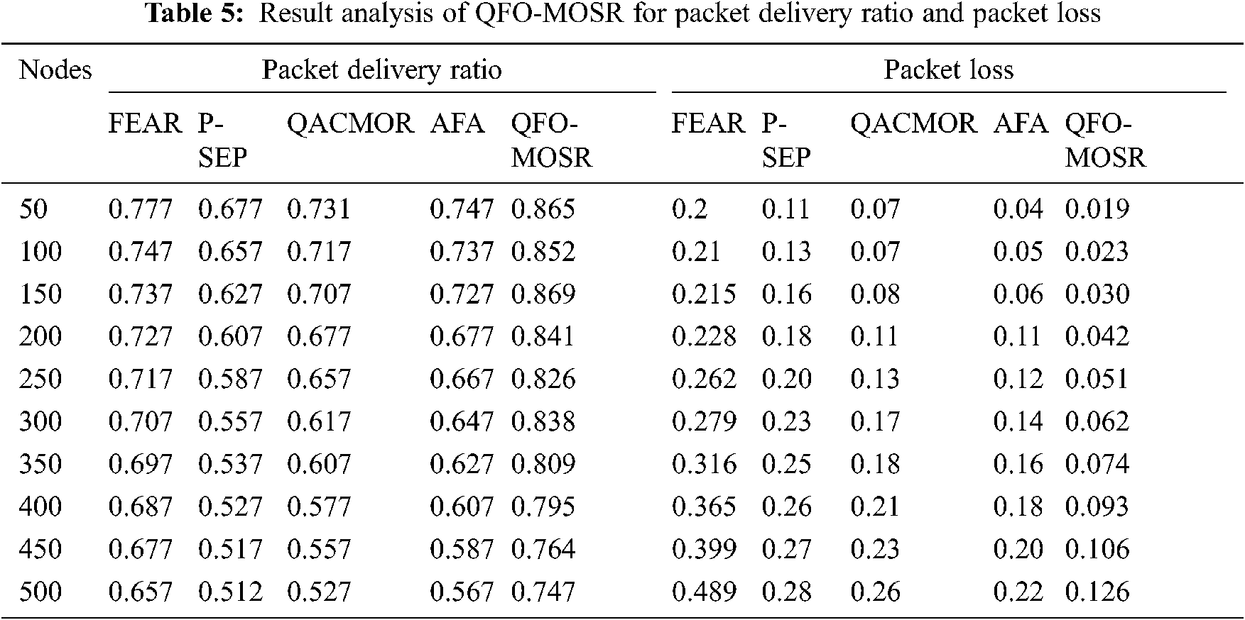
Simultaneously, under 150 nodes, the QFO-MOSR technique has reached a lower packet loss of 0.0308, whereas the FEAR, P-SEP, QACMOR, and AFA models have exhibited higher packet loss 0.215, 0.16, 0.08, and 0.06, respectively. Along with that, under 300 nodes, the QFO-MOSR technique has reached a lower packet loss of 0.0628, whereas the FEAR, P-SEP, QACMOR, and AFA models have exhibited higher packet loss of 0.279, 0.23, 0.17, and 0.14, respectively. Eventually, under 500 nodes, the QFO-MOSR methodology has reached a lower packet loss of 0.1267, whereas the FEAR, P-SEP, QACMOR, and AFA techniques have exhibited higher packet loss 0.489, 0.28, 0.26, and 0.22 correspondingly.

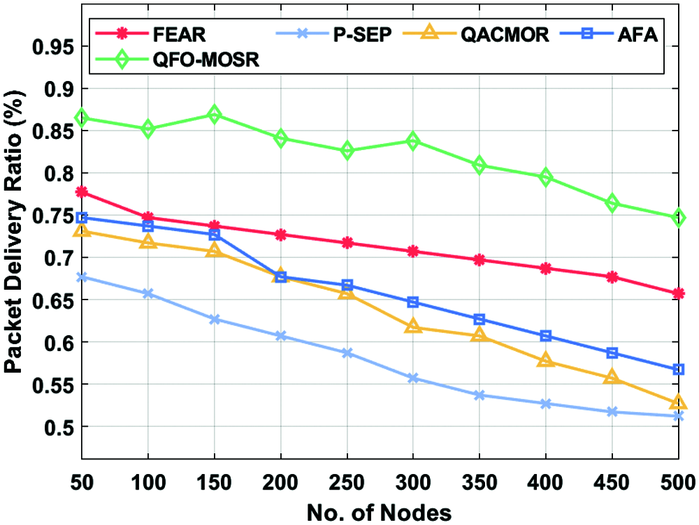
Figure 7: PDR analysis of QFO-MOSR

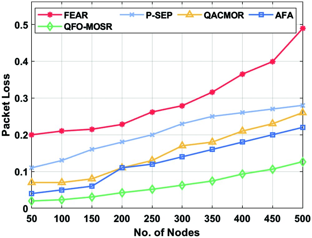
Figure 8: Packet loss analysis of QFO-MOSR

5  Conclusion

This paper has developed an effective QFO-MOSR protocol for Fog-based WSN. The proposed QFO-MOSR protocol derives an optimal set of routes to the destination using a fitness function involving seven parameters. The QFO-MOSR technique is derived from the concepts of quantum computing and the FF optimization algorithm. The proposed routing technique derives a fitness function including trust factor from ensuring security. To investigate the effectual outcome of the QFO-MOSR technique, simulations occur, and results are examined under diverse dimensions. The experimental analysis ensured that the QFO-MOSR technique is superior to other methods in terms of different measures. Therefore, it can be employed as an effective tool in several real-world applications. As a part of future work, the secrecy of the Fog-bases WSN can be guaranteed using the design of deep learning-based intrusion detection methodologies.

Funding Statement: The authors received no specific funding for this study.

Conflicts of Interest: The authors declare that they have no conflicts of interest to report regarding the present study.

This work is licensed under a Creative Commons Attribution 4.0 International License, which permits unrestricted use, distribution, and reproduction in any medium, provided the original work is properly cited.