DOI:10.32604/iasc.2022.020746
| Intelligent Automation & Soft Computing DOI:10.32604/iasc.2022.020746 | |
| Article |
Constructing a Deep Image Analysis System Based on Self-Driving and AIoT
1Department of Electrical Engineering, National Chin-Yi University of Technology, Taichung, 411030, Taiwan
2Department of Information Technology, Takming University of Science and Technology, Taipei City, 11451, Taiwan
*Corresponding Author: Sung-Jung Hsiao. Email: sungjung@gs.takming.edu.tw
Received: 06 June 2021; Accepted: 12 July 2021
Abstract: This research is based on the system architecture of Edge Computing in the AIoT (Artificial Intelligence & Internet of Things) field. In terms of receiving data, the authors proposed approach employed the camera module as the video source, the ultrasound module as the distance measurement source, and then compile C++ with Raspberry Pi 4B for image lane analysis, while Jetson Nano uses the YOLOv3 algorithm for image object detection. The analysis results of the two single-board computers are transmitted to Motoduino U1 in binary form via GPIO, which is used for data integration and load driving. The load drive has two parts: DC motor (rear wheel drive) and servo motor (front wheel steering). Then the final data of NodeMCU is wirelessly transmitted to the router, and then transmitted to the terminal smart device through the 4G network, thus completing the task of monitoring automatic driving. At present, artificial intelligence, the Internet of Things, and autonomous driving technologies are developing rapidly. The highlights of this research are three parts. The first part is the use of two image analysis methods to complete the automatic driving work, and the second part is the hardware architecture and circuit combination. The third part is that the system of this research is designed based on the Internet of Things architecture. The proposed system is to realize the data integration of various analysis platforms such as Raspberry Pi 4B, Jetson Nano, Motoduino U1, and mobile phone APP. The proposed method can not only realize the driving of an autonomous driving model car through image analysis but also monitor the autonomous driving process.
Keywords: AIoT; edge computing; single-board computer; image lane analysis; image object detection
In recent years, artificial intelligence, Internet of Things, and Self-Driving Car technology have flourished. It can solve many problems that humans are facing, such as traffic safety, wasted commuting time, traffic flow, insufficient parking spaces. If self-driving cars are sold to consumers when the technology is immature, the entire society will be harmed, not just the driver. Therefore, this research still has a long way to go to achieve fully automated driving [1].
According to the standards of the Society of Automotive Engineers (SAE), six levels of autonomous driving technology are stipulated. At present, the level that human development can touch falls on the second and third levels. In the second level, the driver mainly controls the vehicle, but the auxiliary system on the vehicle allows the driver to reduce the operational burden. In level three, the vehicle can already drive automatically in some situations, but during the self-driving period, the driver is still on standby to control the vehicle. This research wants to work towards the second level of autonomous driving [2].
Autonomous driving has two technical meanings, “Wisdom” and “Ability”. “Wisdom” corresponds to environmental sensing and decision-making plans, and the motor and mechanical control of the vehicle shows its “Ability” part. The current mainstream external sensors include cameras, lidars, ultrasonic radars, and positioning systems. These sensors can provide huge driving environment data. In this study, the system receives two data from the camera and ultrasonic radar as environmental parameters. If you want to effectively use the data returned by the sensor; you need to combine different data based on some criteria [3].
Currently in the IoT field, Google, Amazon, IBM, etc. are committed to development environment that can write neural networks on the cloud. Since the personal computer hardware used by many people cannot withstand the tasks of their own training, if the neural network is trained in the cloud, there will be no hardware problems, and it can help customers who need a lot of calculations. However, this research focuses on real-time image analysis. If you want to analyze each image in the cloud and return the result to the terminal device, it will cause severe attenuation and consume a lot of power on the radio. Computer vision analysis is a busy job, so using Edge Computing [4] as the system architecture, as shown in Fig. 1. It can not only instantly return the machine execution status, but also enable testers to provide a more secure monitoring environment.
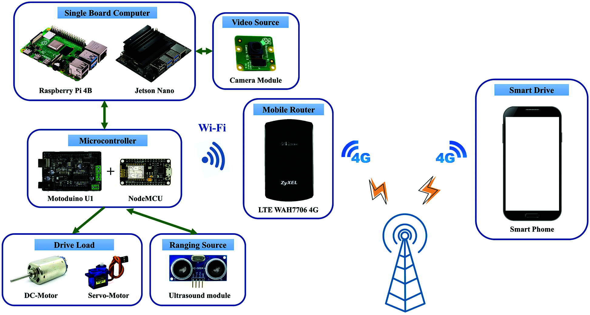
Figure 1: Architecture of system
Petrov et al. published the NB-IoT system in-vehicle driving [5], and Shafique et al. published IoT related to 5G architecture [6]. Minovski et al. studied the IoT application of Autonomous Vehicles [7]. Gao proposed using parallel interpolation to enhance the safety of autonomous driving [8]. Mourad et al. published on Ad Hoc vehicular fog enabling cooperative low-latency intrusion detection [9]. Mamdouh et al. proposed a deep learning framework based on YOLO (You Only Look Once) technology [10]. Tourani et al. showed a robust deep learning approach for automatic Iranian vehicle license plate detection and recognition [11]. Li et al. used YOLOv3 technology to detect ships from images [12]. Liu et al. published the use of edge computing in the Internet of Things and 5G networks [13]. Donno et al. compared IoT, cloud, fog, and edge computing in related research [14]. Goudarzi and others also published edge computing under the framework of the Internet of Things [15].
Fig. 2 shows Self-driving realization and monitoring flowchart. In the beginning, the flowchart is divided into two modules: “Camera module read image” and “ultrasonic module reads the measurement distance”. The hardware part is divided into “Raspberry Pi 4” and “Jetson Nano”. The Raspberry Pi 4 is used for video analysis, while Jetson Nano is used for object detection in deep learning.
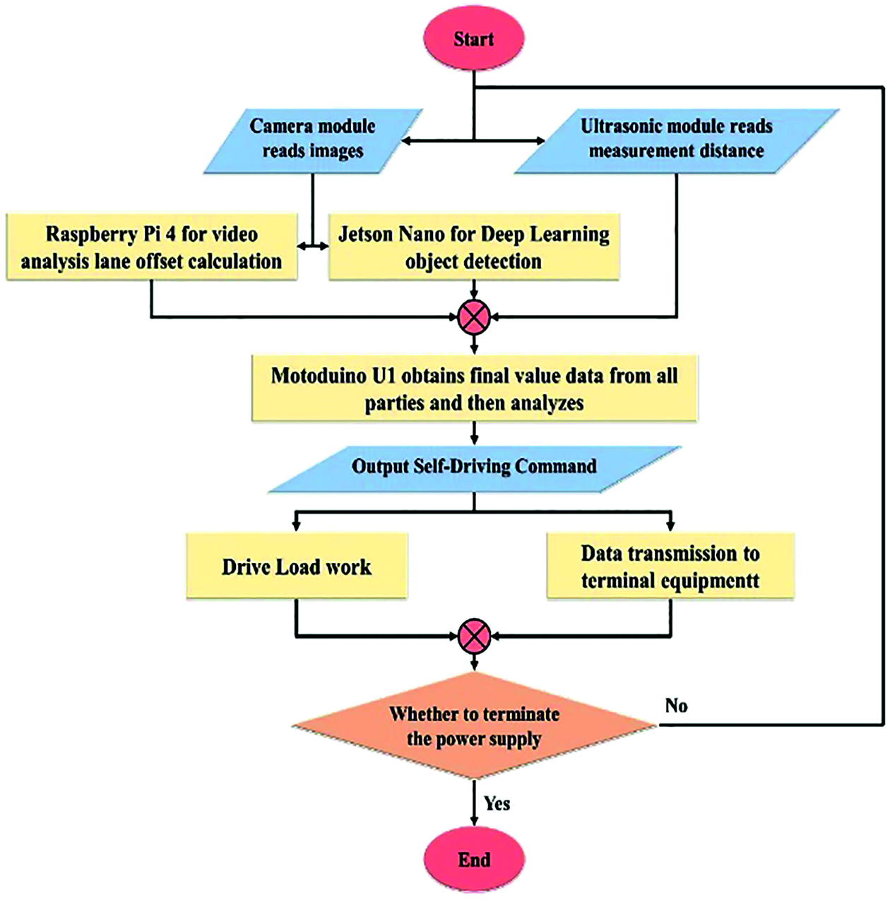
Figure 2: Self-driving realization and monitoring
Raspberry Pi is a single board computer developed by the Raspberry Pi Foundation in the United Kingdom. The main purpose of this plan is to provide low-cost hardware and integrate software resources for education and development. Raspberry pi 4 model b is the latest product in the raspberry pi single-board computer series, as shown in Fig. 3a. The operating system is Raspbian. Specifically, it includes Python, Scratch, Sonic Pi, Java and several other important software packages [16,17].

Figure 3: (a) Raspberry pi 4 model b; (b) Jetson Nano; (c) 8MP raspberry pi camera module (v2); (d) NodeMCU v2
Features of raspberry pi 4 model b:
• A 1.5 GHz quad-core 64-bit ARM Cortex-A72 CPU.
• 4GB of LPDDR4 SDRAM.
• Full-throughput Gigabit Ethernet.
• Dual-band 802.11ac wireless networking.
• Bluetooth 5.0.
• Two USB 3.0 and two USB 2.0 ports.
• Dual monitor support, at resolutions up to 4 K.
• VideoCore VI graphics, supporting OpenGL ES 3.x.
• 4Kp60 hardware decode of HEVC video.
NVIDIA Jetson is an artificial intelligence platform designed by NVIDIA for embedded systems. As shown in Fig. 3b, the Jetson Nano with a size of only 70 × 45 mm is the smallest single-board computer in the Jetson series. However, it has a computing power of 472 GFLOP, which enables it to simultaneously perform multiple neural networks, image classification, and Target detection, voice processing, and the work process only needs 5 to 10 watts of power. When AI technology is deployed on these edge devices, it has huge advantages for modular system production [18]. In this research, the proposed method uses it to build the YoLov3 algorithm to enable self-driving cars to recognize objects.
Features of Jetson Nano:
• GPU: 128-core NVIDIA Maxwell™ architecture-based GPU.
• CPU: Quad-core ARM A57 @ 1.43 GHz.
• Video: 4 K @ 30 fps (H.264/H.265)/4 K @ 60 fps (H.264/H.265) encode and decode.
• Camera: 2x MIPI CSI-2 DPHY lanes.
• Memory: 4 GB 64-bit LPDDR4 25.6 GB/s.
• Connectivity: Gigabit Ethernet.
• Size: 69 mm × 45 mm.
The official Raspberry Pi High Definition (HD) camera can be connected to any single-board computer. It uses Sony’s IMX219PQ image sensor to create high-definition images and still photos, as shown in Fig. 3c. This research uses it to receive video sources.
Features of camera module:
• Resolution: 8,000,000 pixels.
• Still picture resolution: 3280 × 2464.
• Max image transfer rate: 1080p30: 720p60; 640 × 480p90.
• Interface: 15 Pin MIPI Camera Serial Interface (CSI-2).
• Lens size: 1/4”.
• Dimensions: 23 × 25 × 9 mm.
Motoduino U1 is a combination development board that integrates Arduino UNO and L293D motor driver chip, as shown in Fig. 4. The chip can drive two DC motors and use the PWM function to control the motor speed. Compatible, most can use all expansion boards stacked on Arduino. This approach uses it to control and analyze the work between various hardware modules.

Figure 4: Motoduino U1
Features of Motoduino U1:
• Can drive two 7 V ~ 12 V motors.
• Working current per channel <= 600Ma.
• Pin 5 and Pin 6 control the speed, and Pin 10 and Pin 11 control the forward and reverse rotation, especially for driving the motor.
• Fully compatible with Atmega16U2 & Atmega328P.
• Provide independent or shared board power drive motor.
• Lead D2 and A0 pins, can be used with extended applications.
NodeMCU v2 is a development board manufactured by Ai-Thinker, as shown in Fig. 3d. It is paired with Espressif ESP8266 ESP12 Wi-Fi module and is compatible with Arduino peripheral pins, so it can support Arduino sensors. It is cheap, simple to operate and easy to obtain. It has become the most popular choice in IoT applications. This paper uses serial communication Tx (transmit) and Rx (receive) to complete the data transmission work with Motoduino U1, then receive all its data, and then select the value to be uploaded. The process uses HTML grammar to write the web page and finally transmits it to the router [19].
Features of NodeMCU v2:
• There are 13 GPIOs that support peripheral functions such as PWM, I2C, UART, SPI, and 10-bit ADC, but no DAC function.
• The CPU selects the 32-bit Tensilica Xtensa LX3, and the processing speed is 80 MHz.
• ROM/RAM provides 64 K Boot ROM, 64 K Instruction RAM and 64 K Data RAM.
• Support Wi-Fi 802.11b/g/n 2.4G Radio, can be set to various network application modes such as AP, Station or AP + Station.
• The USB to TTL chip of NodeMCU Lua v2 has been replaced by the more stable SiLab CP2102, which can be plug and play.
The authors employed the mobile router as shown in Fig. 5a. This system can receive the data sent by NodeMCU via Wi-Fi, and then transmit it to the terminal device via 4G. Because it will move with the vehicle, I chose a mobile router, which is equipped with a lithium battery, and the electric car will be charged at the same time when it starts.

Figure 5: (a) LTE WAH7706 4G; (b) DC motor; (c) SG-90 9G; (d) HC-SR04
DC motor is the simplest motor, as shown in Fig. 5b. In this type of motor, when current flows through a coil placed in a fixed magnetic field, a magnetic field is generated around the coil. Since each coil is pushed away by the same pole of the fixed magnetic field and attracted by the opposite pole, the coil assembly rotates. In order to maintain the rotation state, the current must be continuously reversed, the polarity of the coil should be continuously reversed, and the coil constantly “chased” the fixed magnetic pole of the opposite sex. By contacting the fixed conductive brush with the rotating commutator, the coil is powered, and the rotation of the commutator causes a reverse current through the coil. Commutators and brushes are the key components that distinguish brushed DC motors from other types of motors. This paper uses it to drive the rear wheels.
Servo motors are electrical devices that can push or rotate objects very accurately. If you want to rotate and at a specific angle, you can use a servo motor, as shown in Fig. 5c. The position of the servo motor is determined by electrical pulses, and its circuit is located next to the motor. Control the servo system by sending electrical pulses of variable width or pulse width modulation (PWM) through the control line. The research uses it to control the steering of the front wheels.
Ultrasonic sensors work by emitting sound waves at a frequency higher than the range of human hearing, and the transducer of the sensor acts as a microphone to receive and send ultrasonic waves. Like many other sensors, our ultrasonic sensors use a single sensor to send pulses and receive echoes. The sensor determines the distance to the target by measuring the time interval between the transmission and reception of ultrasonic pulses, as shown in Fig. 5d. This approach places it on the front of the car and sent the sensed distance back to Motoduino U1.
The proposed approach is that the authors employed a 1:10 remote control car as the car shell, and design and integrate all the hardware circuits, as shown in Fig. 6a. In addition, the venue was constructed with 57 black puzzle pieces and white tape, as in Fig. 6b.

Figure 6: (a) Mini self-driving car (1:10); (b) venues
4 Lane Analysis of the Raspberry Pi 4 Model B
The proposed method creates a C++ development environment in Raspberry Pi, receive images through the camera module, and then perform image lane analysis [20–22]. The analysis process is divided into six steps, as shown in Fig. 7.

Figure 7: Lane analysis image
In this step, this research captures the image of the front of the vehicle by receiving the Raspberry Pi camera module, as shown in Fig. 8a. Since this method only needs to analyze a part of the lane, the system eliminates the rest. The image is generated by creating a quadrilateral using red and orange lines, and then the area of the quadrilateral will be analyzed.

Figure 8: (a) Create region of lanes; (b) perspective transformation
4.2 Perspective Transformation
Perspective Transformation is to project the picture to a new Viewing Plane, also known as Projective Mapping, as shown in Fig. 8b. The transformation formula is:
The transformed coordinates x and y are:
The transformation matrix can be split into 4 parts; this means linear transformations, such as scaling, cutting and broaching:
This matrix is used for Panning:
This matrix is used to generate the perspective transformation:
The perspective-transform image is usually not a parallelogram unless the mapping view plane is parallel to the original plane. Rewriting the previous conversion formula can get:
Therefore, the transformation formula can be obtained by knowing several points corresponding to the transformation. Conversely, specific conversion formulas can also be used for new converted pictures. From the image captured in the previous step, this approach finds the range of the lane through the perspective conversion function. The converted image looks like a bird’s eye view of the quadrilateral area, the proposed approach can clearly see the rest of the image is deleted, only the lane area is concentrated, this conversion will help the calculation.
The conversion of color image to grayscale image is very widely used in image processing, and many algorithms are only effective for grayscale image, so grayscale conversion is a very important link, as shown in Fig. 9a. RGB (Red, Green and Blue) is a space defined by the colors recognized by the human eye and can represent most colors. But in scientific research, RGB color space is generally not used, because its details (hue, brightness, saturation) are difficult to digitally adjust. The X, Y and Z axes are established in the Cartesian coordinate system by the R, G and B axes. The color of each pixel can be represented by a point in three-dimensional space, and the color of each pixel of the Gray graph can be represented by a straight line R = G = B to indicate a point. Therefore, the essence of RGB to grayscale is to find the conversion between three-dimensional space and one-dimensional space. There is a very famous psychological formula:

Figure 9: (a) Gray; (b) threshold operation
According to this formula, the R, G, and B values of each pixel are sequentially read, the gray value is calculated, and the gray value is assigned to the corresponding position of the new image. Traverse all pixels once to complete the conversion.
After converting the image to grayscale, all pixels of each grid point are between 0–225, and this method defines a value to perform threshold calculation for each pixel, as shown in Fig. 9b. When the pixel is smaller than the threshold, it is 0, and when the pixel is larger than the threshold, it is 225. Through many experiments, this system sets the threshold to 200. The proposed approach uses edge detection in image processing later. For this reason, the following Canny calculus does use two thresholds.
After the threshold operation, Canny edge detection is performed in this step, as shown in Fig. 10a. Which are mainly performs the following four operations:

Figure 10: (a) Canny edge detection; (b) calibration using histogram and vector
The realization of image Gaussian filtering can be realized by weighting two one-dimensional Gaussian kernels twice, or by convolution of one two-dimensional Gaussian kernel. This formula is a discrete one-dimensional Gaussian function, and one-dimensional kernel vector can be obtained by determining the parameters:
This formula is a discrete two-dimensional Gaussian function, and the two-dimensional kernel vector can be obtained by determining the parameters:
Gaussian filtering of the image is actually based on the gray value of the predetermined point to be corrected and its neighboring points, and averaged according to certain parameter rules, which can effectively filter out high-frequency noise in the ideal image.
4.5.2 Magnitude and Direction of the Gradient
The first-order finite difference can be used to approximate the image gray value gradient, so that two matrices of partial derivatives of the image in the x and y directions can be obtained. The convolution operators used in the Canny algorithm are as follows:
The mathematical expression for calculating the gradient size and gradient direction is:
where f is the image gray value, P represents the gradient amplitude in the X direction, Q represents the gradient amplitude in the Y direction, M is the amplitude of the point, and θ is the gradient direction and angle.
4.5.3 Non-Maximum Suppression of Gradient Amplitude
The larger the element value in the image gradient amplitude matrix, the larger the gradient value of the point in the image, but this does not mean that the point is an edge; it is only a process of image enhancement. In the Canny algorithm, non-maximum suppression is an important step in edge detection. It means to find the local maximum value of the pixel and set the grayscale value corresponding to the non-maximum point to 0, so as to eliminate most of the non-edge points, but such a detection result still contains a lot of noise and other Causes of false edges, so further processing is needed.
4.5.4 Dual Threshold Algorithm
The method to reduce the number of false edges in the Canny algorithm is to use the double threshold method. The method for selecting dual thresholds is to select the highest grayscale value among the first 80% grayscale values in the order of grayscale values of each image from low to high, and the low threshold is half of the high threshold. The edge image is obtained according to a high threshold. Such an image has almost no false edges, but due to the high threshold, the resulting image edges may not be closed. So in order to solve this problem, another low threshold is used. In a high-threshold image, the edge is linked as a contour. When the end of the contour is reached, the algorithm will find a point that meets the low threshold among the 8 neighboring points of the breakpoint, and then collect a new edge according to the point until the image the entire edge is closed.
4.6 Calibration Using Histogram and Vector
In this operation, the system draws four lines in the previous image conversion results, as shown in Fig. 10b. Each line represents a different meaning:
• Purple line: left lane.
• Yellow line: right lane.
• Green line: calculate the centerline of the lane based on the purple line and the yellow line.
• Blue line: the centerline of the front camera.
Use the difference between the blue line and the green line to calculate the offset between the car and the lane. When the two lines are close to overlap, it means that the direction of the car is straight, and the output value is close to 0. When the green line moves to the right and left, the blue line calculates the offset value according to the offset from the green line. To the left, the output value is larger, and the green line is to the right, the output value is smaller. These values can provide the required steering angle information for the front wheels.
5 Object Recognition of the Jetson Nano
At present, deep learning has two mainstream schools in object detection, candidate frame method and regression method. The candidate frame genre mainly uses a certain algorithm to obtain the candidate image area where the object is located, and then classifies this area, represented by Faster RCNN, SPP, and R-FCN. The regression method is mainly to directly perform BBox (Bounding Box) regression and subject classification; it is represented by YOLO and SSD. The concept of IOU (Intersection Over Union) is often used in target detection to indicate the degree of overlap of two rectangular boxes, that is, the area of their intersecting part is divided by the area of their merged part. The larger the value, the more overlap. It’s more accurate the detection, as shown in Fig. 11 [23–24].

Figure 11: Intersection over union calculation
There are currently three mainstream object detection algorithms, such as Faster RCNN, SSD, and YOLO. Although our experiments show that Faster RCNN has the highest detection accuracy, its detection speed is also the slowest. Although the YOLO algorithm has the lowest detection accuracy, its detection speed is the fastest. We know that the car is a high-speed moving object, and automatic driving technology is very important for the detection speed requirements. In addition, our research is used for the realization of the object detection computer is Jetson Nano, it is a computer that can barely withstand a large number of graphics calculations the single-board computer is limited, so the object detection algorithm suitable for it is also limited. Finally, our research chose to use YOLO as the reason for the object detection algorithm.
YOLO literally means “You Only Look Once”, and the problem can be solved by just seeing it once. There are currently three versions of YOLO: YOLOv1, [25] YOLOv2, [26] YOLOv3 [27]. The core idea of YOLO is to directly output the entire picture to BBox location information and classification information through a neural network. The final output will be divided into S × S grids. If the center of a real subject falls in these grids, then these grids will be responsible for detecting this subject. This grid generally predicts B number of BBoxes. Each BBox contains position information and Confidence. Using Pr (Object) × IOU, it expresses the presence or absence of the subject and the accuracy of the BBox. Pr (Object) = 1 when there is a body, Pr (Object) = 0 when there is no body. IOU will predict the IOU value between the BBox and the real BBox. For categories, operations similar to Softmax will be done. If there are C main categories, then a grid will output (5 × B + C) pieces of information, and the output of all grids is S × S × (5 × B + C) Amount.
Each YOLO grid is only responsible for the detection and recognition of one subject. Because CNN has a sampling process, the resolution will gradually decrease. Therefore, when the two subjects are very close and the subjects are particularly small, the effect of YOLO is it can’t be so good. Of course, this is also a challenge that all object detection algorithms will encounter. In order to enhance the detection accuracy and recall rate, YOLOv2 appeared. It strengthens the resolution of training images, and at the same time quotes the idea of Anchor box in Faster RCNN, and designs the Darknet-19 classification network architecture. The Anchor box in YOLOv2 is different from the manual setting in Faster RCNN. It will perform K-Means clustering on the marked real BBox and automatically analyze the representative Anchor box. In addition, YOLOv2 uses a cross-layer transfer method similar to ResNet to increase fine-precision features. Multi-scale images are also used for training, from 320 to 608, which are multiples of 32. Because the sampling multiple is 32, this ensures that the output is shaped.
The Darknet-19 classification network architecture is shown in Fig. 12a. It mainly uses 3 × 3 pooling to double the number of channels, then uses 1 × 1 convolution to reduce the number of channels, and finally uses global average pooling to replace the full connection in the YOLOv1 version. Do predictive classification. The detection network is to remove the last 1 × 1 convolutional layer of the classification network, and then connect three 3 × 3 core 1024 output channels of the convolution layer, and then connect the number of categories of 1 × 1 convolution layer. Each Anchor box in YOLOv2 will be responsible for its own location information, confidence value and category probability, which are different from YOLOv1. YOLOv2 is faster than Faster RCNN and SSD, but the sacrifice is accuracy.

Figure 12: (a) Darknet-19 structure; (b) darknet-53 structure; (c) MS COCO dataset
YOLOv3 was published in 2018, mainly for the detection of small objects, and the results are also very robust, quickly solving the problem of small objects. YOLOv3 uses multiple independent Logistic classifiers to replace the Softmax classifier in YOLOv2. Anchor boxes are grouped into nine groups instead of five in the YOLOv2 version, and each scale predicts three BBoxes. The basic network uses Darknet- 53, as shown in Fig. 12b. Its advantages are high efficiency, low background false detection rate, and strong versatility, but its disadvantages are still low accuracy and recall.
5.2 YOLOv3 Model Configuration
The default training data set by YOLO is Microsoft COCO, and there are 80 object tags in the COCO data set, as shown in Fig. 12c. If you only need to detect common objects, such as people, chairs, backpacks, umbrellas, you can use this data set for training, which can also save a lot of time. In this study, the system only needs to detect three objects first, namely people, car, and stop signs. First, this system copies the yolov3.cfg file in the cfg, directory and rename it to self_driving_car_ yolov3.cfg, and then start to set the contents inside. This research modifies the parameters of the YOLO layer and changes the number of categories to 3. In addition, the Filters parameter in the Convolutional layer above the YOLO layer must be changed to 24, because the calculation formula for this parameter is:
So if there are 3 objects, the formula is calculated as:
If training with the COCO dataset, the calculation of this parameter is as follows:
In the application, please pay attention to modify according to the actual situation. Next, set the category name file, create a new file self_driving_car. names in the data/directory to save the category name, the contents of the file are: car, person, and stop sign. Then configure the file and create a new file self_driving_car.data in the cfg/directory. The content is as follows: classes = 3, train = /path/to/train.list, valid = /path/to/val.list, names = data/cat_and_dog.names, backup =backup/. Finally, after downloading the pre-trained weight file, you can start training. After the training is complete, you will get the weight file self_driving_car_yolov3_final. A weight is in the backup/directory. First, set both batch and subdivisions in the self_driving_car_yolov3.cfg file to 1, so that object detection can be performed.
The object detection results are shown in Figs. 13a and 13b. First, after the objects detected by the image are classified, a rectangle is drawn on the periphery of the object, and the label of the classified object and the confidence level are marked on the top of it.

Figure 13: (a) Identify person and cars; (b) identify stop signs; (c) App display
6 Smart Terminal Display Results
Finally, this system transfers the data to the APP. Since the content displayed by the APP is not much, this research uses MIT APP Inventor for production, as shown in Fig. 13c. The interface has five main contents. The remote image is captured to the web page through Raspberry Pi 4B and displayed through the hyper-connected module. Displays the lane offset data analyzed by Raspberry Pi 4B. The farther to the left, the more positive the value, the farther to the right, the more negatives the value, and the closer to straight the value is close to zero. Display the classified objects analyzed by Jetson Nano. Through Wi-Fi wireless transmission, it can be used to manually control the buttons of the vehicle. Autopilot switch mode button. In this way, the edge computing analysis method is completed, and our image analysis process is performed on the edge device. The terminal device will only receive the final value analyzed by the edge device without discussing the process.
This research has described the detailed analysis process in the lane analysis process. In this research, authors have described how to build a predictive model and basic principle structure in the process of object detection. The following list shows the recognition error rate encountered by autonomous vehicles. In the study, it will increase once when the autonomous vehicle runs a lap of the track. Tab. 1 shows recognition rate in various situations.
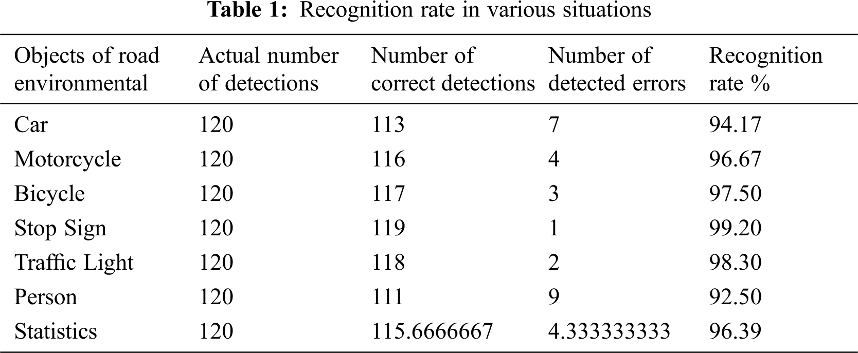
The image analysis process of the authors’ research is real-time detection. Since the analysis environment is a customized mini model, the source of accuracy will depend on the image data set collected by our research. The figure below shows the identification rate analysis of object detection. It will accumulate once every time it ran. The authors will test each object 120 times as the standard. You can see that the more the number of wrong identifications of the object, the more the identification rate is. The lower it is, although its recognition rate in humans is 92% on average, its performance in the overall autonomous driving research is as high as 96%, so it meets our expectations. Fig. 14 presents the recognition rate analysis of object detection.

Figure 14: Recognition rate analysis of object detection
The proposed system is composed of multiple microcontrollers, which results in a slight compatibility error when the system software analyzes the road condition identification. But these errors can be corrected by software, so that the simulated driving of the system is consistent with the real driving. Therefore, when automakers are developing new cars with autonomous driving, they can first adopt our simulated autonomous driving system. The advantage of artificial intelligence is that it can be repeatedly trained in the virtual world. When the virtual automatic driving error rate reaches a safe low value, the system can be applied to the real world of self-driving cars. Compared with the traditional way to develop an automatic driving system, the method proposed in this paper will be a way to save production cost.
Since cars are expensive items, it is impossible to really buy a car to test autonomous driving tasks. The authors reduced the ratio of 1:10 to simulate the car and the field for testing. During the authors’ research, apart from learning about the current development of autonomous driving, the authors also discovered that some problems need to be overcome in the future. First of all, because the technology the authors mainly use is image analysis and ultrasonic ranging, the site can only design one track instead of complicated. If the authors need to get from one point to another, the authors need to create a virtual map and positioning system, such as Google Map. Without these systems, the authors would not be able to complete navigation. From this point, the authors can see that the professional knowledge required in the field of autonomous driving is very extensive. If the number of people is small, the scope of research will be limited. It takes teamwork to gather talents from different professional fields to construct a complete autonomous driving system.
The second point is that when simulating lane recognition on the raspberry pi, it is also found that if the road is uneven and the lane line is unclear, it is easy to analyze errors. Only then did the authors realize that if mankind wants to continue to develop autonomous driving technology in the future, it must cooperate with the national road planning. Otherwise, it will be difficult to make correct judgments if the road planning is poor. The authors think because the current traffic rules are designed based on human driving as a starting point, if autonomous driving wants to enter human society in the future, the traffic rules may also be changed. The third point is that when doing object detection research on Jetson Nano, the authors was very happy when Stop Sign was detected, but when the authors calmed down and thought about it, the authors found a problem. Why do the authors need to recognize traffic signs? Now when this system is driving a car, this system is watching various traffic signs through our eyes and then reacting, but in the future, it should be unnecessary for autonomous driving machines with positioning systems and map information. Because no matter it is traffic light, stop sign, speed limit, the authors have already put it in the map data. This way, in addition to reducing the burden of image analysis, the authors can also learn more accurately the road conditions of the current location.
The future research direction the authors want to start towards the map positioning system. If the authors want to create my own analog map, the authors should start with indoor positioning, so that in addition to navigation, the road information displayed on the terminal will be richer and more complete.
Acknowledgement: This research was supported by the Department of Electrical Engineering at National Chin-Yi University of Technology. The authors would like to thank the National Chin-Yi University of Technology, Takming University of Science and Technology, Taiwan, for supporting this research.
Funding Statement: The authors received no specific funding for this study.
Conflicts of Interest: The authors declare that they have no conflicts of interest to report regarding the present study.
Availability of Data and Materials: Data sharing not applicable to this article as no datasets were generated or analyzed during the current study.
1. Q. Rao and J. Frtunikj, “Deep learning for self-driving cars: Chances and challenges,” in Proc. SEFAIAS, Gothenburg, Sweden, pp. 35–38, 2018. [Google Scholar]
2. A. Ndikumana, N. H. Tran, D. H. Kim, K. T. Kim and C. S. Hong, “Deep learning based caching for self-driving cars in multi-access edge computing,” IEEE Transactions on Intelligent Transportation Systems, vol. 22, no. 5, pp. 2862–2877, 2021. [Google Scholar]
3. R. Buyya and S. N. Srirama, Fog and Edge Computing: Principles and Paradigms, New York, NY, USA, John Wiley & Sons, 2019. [Google Scholar]
4. W. Vanderbauwhede and J. Singer, Operating Systems Foundations with Linux on the Raspberry Pi: Textbook, UK, Arm Education Media, 2019. [Google Scholar]
5. V. Petrov, A. Samuylov, V. Begishev, D. Moltchanov, S. Andreev et al., “Vehicle-based relay assistance for opportunistic crowdsensing over narrowband IoT (NB-IoT),” IEEE Internet of Things Journal, vol. 5, no. 5, pp. 3710–3723, 2018. [Google Scholar]
6. K. Shafique, B. A. Khawaja, F. Sabir, S. Qazi and M. Mustaqim, “Internet of things (IoT) for next-generation smart systems: A review of current challenges, future trends and prospects for emerging 5G-IoT scenarios,” IEEE Access, vol. 8, pp. 23022–23040, 2020. [Google Scholar]
7. D. Minovski, C. Åhlund and K. Mitra, “Modeling quality of IoT experience in autonomous vehicles,” IEEE Internet of Things Journal, vol. 7, no. 5, pp. 3833–3849, 2020. [Google Scholar]
8. K. Gao, B. Wang, L. Xiao and G. Mei, “Incomplete road information imputation using parallel interpolation to enhance the safety of autonomous driving,” IEEE Access, vol. 8, pp. 25420–25430, 2020. [Google Scholar]
9. A. Mourad, H. Tout, O. A. Wahab, H. Otrok and T. Dbouk, “Ad hoc vehicular fog enabling cooperative low-latency intrusion detection,” IEEE Internet of Things Journal, vol. 8, no. 2, pp. 829–843, 2021. [Google Scholar]
10. N. Mamdouh and A. Khattab, “YOLO-Based deep learning framework for olive fruit fly detection and counting,” IEEE Access, vol. 9, pp. 84252–84262, 2021. [Google Scholar]
11. A. Tourani, A. Shahbahrami, S. Soroori, S. Khazaee and C. Y. Suen, “A robust deep learning approach for automatic Iranian vehicle license plate detection and recognition for surveillance systems,” IEEE Access, vol. 8, pp. 201317–201330, 2020. [Google Scholar]
12. H. Li, L. Deng, C. Yang, J. Liu and Z. Gu, “Enhanced YOLO v3 tiny network for real-time ship detection from visual image,” IEEE Access, vol. 9, pp. 16692–16706, 2021. [Google Scholar]
13. Y. Liu, M. Peng, G. Shou, Y. Chen and S. Chen, “Toward edge intelligence: Multiaccess edge computing for 5G and internet of things,” IEEE Internet of Things Journal, vol. 7, no. 8, pp. 6722–6747, 2020. [Google Scholar]
14. M. D. Donno, K. Tange and N. Dragoni, “Foundations and evolution of modern computing paradigms: Cloud, IoT, edge, and fog,” IEEE Access, vol. 7, pp. 150936–150948, 2019. [Google Scholar]
15. M. Goudarzi, H. Wu, M. Palaniswami and R. Buyya, “An application placement technique for concurrent IoT applications in edge and fog computing environments,” IEEE Transactions on Mobile Computing, vol. 20, no. 4, pp. 1298–1311, 2020. [Google Scholar]
16. J. Cabral and G. Halfacree, The NEW Official Raspberry Pi Beginner’s Guide: Updated for Raspberry Pi 4, Cambridge, UK, Raspberry Pi Trading Ltd., 2019. [Google Scholar]
17. A. Kurniawan, Getting Started with NVIDIA Jetson Nano Kindle Edition, Santa Clara. CA, USA, Nvidia Corporation, 2019. [Google Scholar]
18. S. S. Prayogo, Y. Mukhlis and B. K. Yakti, “The use and performance of MQTT and CoAP as internet of things application protocol using NodeMCU ESP8266,” in Proc. ICIC, Semarang, Indonesia, pp. 1–5, 2019. [Google Scholar]
19. D. M. Escriva, P. Joshi, V. G. Mendonca and R. Shilkrot, Learning Path Building Computer Vision Projects with OpenCV 4 and C++, Birmingham, UK, Packt Publishing, 2019. [Google Scholar]
20. R. Shilkrot and D. M. Escriva, Mastering OpenCV 4: A Comprehensive Guide to Building Computer Vision and Image Processing Applications with C++, Birmingham, UK, Packt Publishing, 2018. [Google Scholar]
21. A. Kaehler and G. Bradski, Learning OpenCV 3: Computer Vision in C++ with the OpenCV Library, New York, NY, USA, O’Reilly Media, 2016. [Google Scholar]
22. F. Chollet, Deep Learning with Python, Shelter Island, NY, USA Manning Publications Co, 2018. [Google Scholar]
23. D. Paul and C. Puvvala, Video Analytics Using Deep Learning: Building Applications with TensorFlow, Keras, and YOLO, New York, NY, USA, Apress, 2020. [Google Scholar]
24. J. Redmon, S. Divvala, R. Girshick and A. Farhadi, “You only look once: Unified, real-time object detection,” in Proc. CVPR, Las Vegas, NV, USA, pp. 779–788, 2016. [Google Scholar]
25. J. Redmon and A. Farhadi, “YOLO9000: Better, faster, stronger,” in Proc. CVPR, Honolulu, HI, USA, pp. 6517–6525, 2017. [Google Scholar]
26. J. Redmon and A. Farhadi, “YOLOv3: An incremental improvement,” in Proc. Computer Vision and Pattern Recognition, Washington, USA, pp. 1–6, 2018. [Google Scholar]
27. M. Jayakumar, Arduino and Android Using MIT App Inventor, Scotts Valley, CA, USA Createspace Independent Publishing Platform, 2016. [Google Scholar]
 | This work is licensed under a Creative Commons Attribution 4.0 International License, which permits unrestricted use, distribution, and reproduction in any medium, provided the original work is properly cited. |