Intelligent Automation & Soft Computing DOI:10.32604/iasc.2022.020461
Article

Multivariate Outlier Detection for Forest Fire Data Aggregation Accuracy

Ahmad A. A. Alkhatib* and Qusai Abed-Al

Alzaytoonah University of Jordan, Amman, 11733, Jordan
*Corresponding Author: Ahmad A. A. Alkhatib. Email: Ahmad.alkhatib@zuj.edu.jo
Received: 25 May 2021; Accepted: 03 July 2021

Abstract: Wireless sensor networks have been a very important means in forest monitoring applications. A clustered sensor network comprises a set of cluster members and one cluster head. The cluster members are normally located close to each other, with overlaps among their sensing coverage within the cluster. The cluster members concurrently detect the same event to send to the Cluster Head node. This is where data aggregation is deployed to remove redundant data at the cost of data accuracy, where some data generated by the sensing process might be an outlier. Thus, it is important to conserve the aggregated data’s accuracy by performing an outlier data detection process before data aggregation is implemented. This paper concerns evaluating multivariate outlier detection (MOD) analysis on aggregated accuracy of data generated by a forest fire environment using OMNeT++ and performing the analysis in MATLAB R2018b. The findings of the study showed that the MOD algorithm conserved approximately 59.5% of aggregated data accuracy, compared with an equivalent algorithm, such as the FTDA algorithm, which conserved 54.25% of aggregated data accuracy for the same event.

Keywords: Wireless sensor network; data aggregation; forest fire; multivariate outlier detection; aggregated data accuracy; MOD

1  Introduction

Wireless sensor networks (WSNs) have been deployed in various fields, including monitoring applications such as forest monitoring, target monitoring, security monitoring and fence monitoring [1]. WSN is grouped into clusters with a cluster head (CH) and number of cluster members (CMs). CMs often generate redundant data, where part of the event data might be outliers caused by data redundancy, errors, noise and missing data [2–4]. To overcome this problem, data aggregation algorithms have been deployed in WSN to remove redundant data and decrease the number of transmissions in the clustered network, but aggregation is performed at the cost of the accuracy of the final aggregated data [1,5]. Accuracy degradation of aggregated data is mainly caused when the CH node receives outlier data. This is important especially in decision-making activity [6] about emergencies such as forest fires.

2  Related Work

Aggregated data accuracy can be conserved when outlier data detection is accomplished before the data aggregation process is implemented. In this regard, there are several outlier data detection algorithms in wireless sensor networks in the literature.

The Fault-Tolerant Data Aggregation (FTDA) algorithm [6] operates within a clustered network. FTDA involves three phases: data collection and locality sensitive hashing (LSH) code generation, outlier detection, redundant data removal and data aggregation. In the data collection phase, the CH node notifies CMs at the beginning of data collection. Each CM detects the event numerous times, stores the transmitted data, and produces an LSH code for the latest transmitted data by random hyperplane-based hash function. The size of the LSH code is smaller than that of the transmitted data. Each CM send its LSH code with a unique ID to the CH node at the end of the data collection session. In the outlier detection phase, the CH node uses the hamming distance between pairs of LSH codes to find the similarity among them. If the similarity of two LSH codes is greater than the similarity threshold, then the MinSupLocal counters at the two related LSH codes are enlarged by 1. If the LSH MinSupLocal counter for a certain LSH is less than the predetermined MinSupLocal threshold, the node that owns this LSH code is an outlier [7].

The CH nodes send the informed messages to the normal nodes to transmit their sensed data. To remove the redundant data, the CH node chooses one CM to transmit its sensed data in case two LSH codes are similar and their MinSupLocal is greater than the MinSupLocal threshold. In the final phase, the CH node aggregates the received sensed data and transmits the aggregation results to the base station [8].

Temporal Data-Driven Sleep Scheduling and Spatial Data-Driven Anomaly Detection for Clustered WSN was proposed by Li et al. [9]. Temporal Data-Driven Sleep Scheduling (TDSS) diminishes the sensor data redundancy for the same node in time sequences, whereas Spatial Data-Driven Anomaly Detection (SDAD) detects outlier or anomalous data and preserves the accuracy of the sensor data for the specific node. The algorithms were applied in a tunnel monitoring system environment to monitor the health of tunnel structure and the duty cycle safety of underground train systems. The clustering topology structure is implemented on the network, in which the CMs transmit the data of an atomic event from diverse types of sensor nodes to the CH node.

The authors proposed SDAD, a cluster network based on anomaly (outlier) detection and employed in the CH node. The authors claimed that SDAD can determine whether the node is operating correctly and is a prerequisite for preserving the accuracy of all sensor data. Anomalies include sensor nodes, “abnormal data” and “discrete nodes”. These anomalies have different data features, such as a small deviation in the “sensor error”, a large deviation in the “abnormal data” and a lack of data in the “node is not connected”. To calculate the data deviation; the difference between the sensor data event and the real data event, the kriging method is employed to estimate the actual data event of the selected node.

Kriging is an admirable spatial interpolation method that can fetch the value of the sensor to an uncontrolled location from near-site monitoring. Kriging makes two main contributions to detect spatial-based anomalies in a tunnel control system. First, kriging takes into consideration the full spatial correlation of the sensor data to achieve high accuracy in spatial completion. Second, kriging applies to a region where sampling data have arbitrary characteristics and structural property. In addition, anomalous detection of spatial data in the tunnel control system is used accurately in this type of area. Whatever is causing “abnormal data”, it can upsurge the anomaly indicator ξ to attract attention. Each sensor node has an anomaly indicator ξ, which is updated once ∆iv1 (subtracting sensory value and real value) is updated, ξ = (ξ + ∆iv1)/2. The anomaly indicator ξ is separated into three levels: green, yellow and red. These levels of anomaly indicators are used to decide the priority level of the node maintenance.

Fault-tolerant multiple event detection in a wireless sensor network was achieved by [8]. The author proposed a polynomial-based scheme that addresses the problems of event region detection (PERD) by having an aggregation tree of sensor nodes. A data aggregation scheme and tree aggregation (TREG) are employed in this study to perform functional approximation of the event using a multivariate polynomial regression. Only the coefficients of the polynomial (P) are passed instead of aggregated data. PERD includes two components: event recognition and event report with boundary detection. This can be performed for multiple simultaneously occurring events. We also identify faulty sensor(s) using the aggregation tree. Performing further mathematical operations on the calculated P can identify the maximum (max) and minimum (min) values of the sensed attribute and their locations. Therefore, if any sensor reports a data value outside the [min, max] range, it can be identified as a faulty sensor. Since PERD is implemented over a polynomial tree on a WSN in a distributed manner, it is easily scalable, and the computation overhead is marginal.

3  System Model

3.1 Wireless Sensor Network Model

The K-means algorithm is the easiest one for generating a clustered WSN due to its ease of implementation, low memory required and computational efficiency [10,11]. In this study, the centralized K-means algorithm was employed to form a clustered WSN. The main purpose is to reduce the workload on the sensor nodes. Also, the BS runs the K-means clustering algorithm, and it decides which nodes are CH and CM. The WSN in this study was divided into clusters. Each CM transmits sensed data to CH, which aggregates them and sends a single data packet to the base station, as shown in Fig. 1.

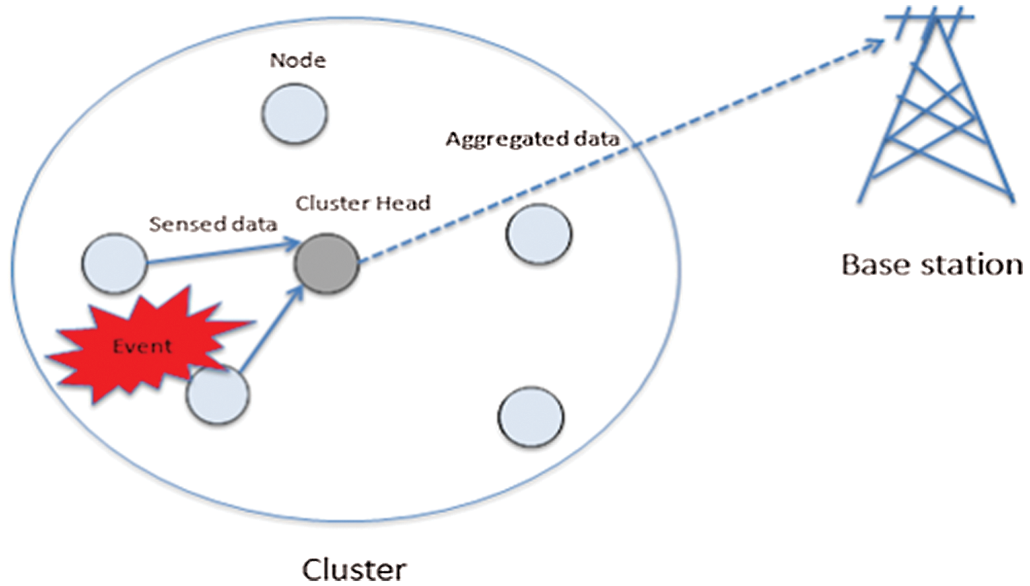
Figure 1: Cluster and aggregated data

However, many steps are considered in the clustered network:

•   The sensor nodes are homogenous and arbitrarily deployed in the area field.

•   Static clustering is employed. Each cluster has a set of limited sensor nodes.

•   Each sensor node has a fixed position.

•   The base station or sink lies outside the boundary of the field area.

•   The sensor node can communicate with the CH by a single-hop communication.

•   CH can communicate with the BS by a single-hop communication.

•   We assume that two composite events occur at the same time in different locations within the cluster.

•   When the event takes place, the CM continuously senses the event until the event becomes hidden or inexistent.

•   The CM node can detect more than one event.

•   We assumed that event 1 involves three attributes–temperature (Temp), light (Light) and smoke (Smoke)–whereas event 2 involves three attributes–accelerate (Accelerate), pressure (Pressure) and carbon dioxide (CO2).

3.2 Data Model

Multivariate normal distribution and standard distribution models were employed in this study. The data values for the event attributes (multivariate) were produced randomly based on a multivariate normal distribution model. In addition, each multivariate normal value was transformed to the standard value.

In the multivariate normal distribution model, a random vector is composed of elements that are normally distributed [12]. Also, a k-dimensional random vector such X = (X1, X2, …, Xk)T is defined as X~N (μ, Σ) [13], where μ is the mean of the normal random vector and Σ is the covariance matrix. The k-dimensional random vector is considered a composite event in WSN. For instance, if there is a 3-dimensional random vector as follows,

V=(XYZ) (1)

The probability density function is of the form,

f(V)=12π|Σ|1/2e−(V−μ)T⁡Σ−1⁡(V−μ) (2)

The expected value E defined as the mean of the normal random vector V is given by

μ=(E(X)E(Y)E(Z))=(μXμYμZ) (3)

where μx is the mean of variable X, whereas μy and μz are the means of the variables Y and Z, respectively. However, the covariance represents an idea of how two random distributed variables are related to each other if they have different units of measurement [14]. The covariance matrix for the normal random vector is given by

Σ=(σX2σXYσXZσYXσY2σYZσZXσZYσZ2) (4)

where σX2 is the variance of the variable X, and σY2 and σZ2 are variance of the variables Y and Z, respectively. The covariance of X and Y variables is represented by σYX . The joint probability distribution (multivariate normal distribution) describes how the entire set of elements of the random vector V takes values together, where μ and Σ are the features of this distribution characterizing the “centre” and “spreading and association” [12,13]. The correlation is a measurement of the linear relationship between the random variables [15]. It is measurement of the association that takes into account the fact that different elements of V may vary differently on their scale [12]. The correlation coefficient between two random variables such as X and Y is given by

Γ=[1ρxyρyx1] (5)

It may be shown that the correlations must satisfy −1 ≤ ρXY ≤ 1. Thus, If ρXY = 1, then σXY = σX σY, whereas if ρXY = 0, then σXY = 0. The correlation matrix for the 3-dimensional random distributed vector V is given by

Γ=(1ρXYρXZρYX1ρYZρZXρZY1) (6)

A) If ρXY = 1, then there is strong correlation between two random variables.

B) If 0 < ρXY < 1, then there is less correlation between two random variables.

C) If ρXY = 0, then the two random variables are independent.

D) If ρXY = −1, then there is strong inverse correlation between two random variables.

E) If −1 < ρXY < 0, then there is less inverse correlation between two random variables.

4  Multivariate Outlier Detection (MOD)

The MOD algorithm will detect outlier data for forest fire events in which a data value is considered an outlier if one or more of its attribute values is an outlier. A multivariate normal distribution model was employed to produce the event attribute values, whereby a bit error rate occurs in the transmission channel. Also, when the attribute values are transformed to the new values, they are called principal components (PCs). The MOD algorithm consists of five steps:

Step 1: The CH node receives actual forest fire event data, which consist of a set of attributes. It is assumed that the forest fire event is a composite event and consists of three attributes (variables), X, Y, Z. Assuming that V is a multivariate normal distribution vector, it includes:

V=(XYZ) (7)

X, Y and Z are random variables that represent the forest fire event attributes, X~N (μx, σx), Y~N (μy, σy) and Z~N (μz, σz), respectively:

Z={z1,z2,z3,...,zn} (8)

The mean of each variable is given by:

μz=∑i=1nzin (9)

where n is the number of variable data values. The standard deviation of each variable is given by:

σz=∑i=1n(zi⁡−μz)2n (10)

Step 2: Transforming each variable X, Y and Z into the standard variables which are given by the following formulas:

SZ=(Z−μz)σz (11)

where SX is the standard of the variable X, whereas SY and SZ are the standard of the variable Y and Z, respectively. (P( SX ) * 100% is the percentage of normal data for the variable SX when its values fall within the interval (−StdCoff, StdCoff), whereas (1 − P( SX ) * 100% is the percentage of false data for the variable SX when its values do not fall within the interval (−StdCoff, StdCoff). These rules are applied to the standard variables SY and SZ too. P( SX ) is the probability of the standard variable SX where Stdcoff is the coefficient times of the standard deviation.

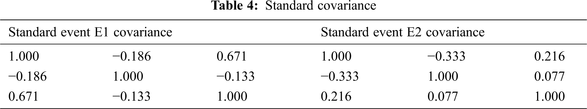
Step 3: Calculating the standard covariance and correlation matrices, in which the mean and the standard deviation for each standard variable are 0 and 1, respectively:

Σ=(σSX2σSX⁡SYσSX⁡SZσSY⁡SXσSY2σSY⁡SZσSZ⁡SXσSZ⁡SYσSZ2) (12)

Γ=(1ρSX⁡SYρSX⁡SZρSY⁡SX1ρSY⁡SZρSZ⁡SXρSZ⁡SY1) (13)

where σSY⁡SZ is the standard covariance between SY and SZ standard variables, and Σ is the standard covariance matrix. ρSY⁡SZ is the standard coefficient correlation between SY and SZ standard variables, whereas Γ is the standard coefficient correlation matrix.

Step 4: Calculating Eigenvalues (λ) and Eigenvectors (U) for the standard correlation matrix. Let us assume that Γm * n is the standard correlation matrix, where each standard variable mean equals 0 and the standard deviation equals 1. Assuming that [λ1, λ2 … λn,] are the Eigenvalues of the standard correlation matrix Γ, the Eigenvalues are none negative and can be ordered such as λ1 ≥ λ2… ≥ λn. Assuming that U = [U1, U2 … Un] are the Eigenvectors of the standard correlation matrix Γ, these Eigenvectors correspond to the ith-largest Eigenvalue. Consequently, the transformed data matrix is given by:

Γ′=ΓU (14)

where Γ′ is the transformed data matrix that contains all new PCs. Each PC value is related to the composite value of SX , SY and SZ together.

Step 5: Find the column of PCs which has the maximum variance of Γ′ and examine each PCi value based on the following function:

f(Pci)={1−Stdcoff≤Pci≤Stdcoff0other} (15)

In the study, the coefficient times of the standard deviation (Stdcoff) determine the number of normal data values that should be aggregated. However, the result of f(Pci) is either 1, which means the composite value (xi, yi, zi) is normal, or 0, which means the composite value (xi, yi, zi) is an outlier.

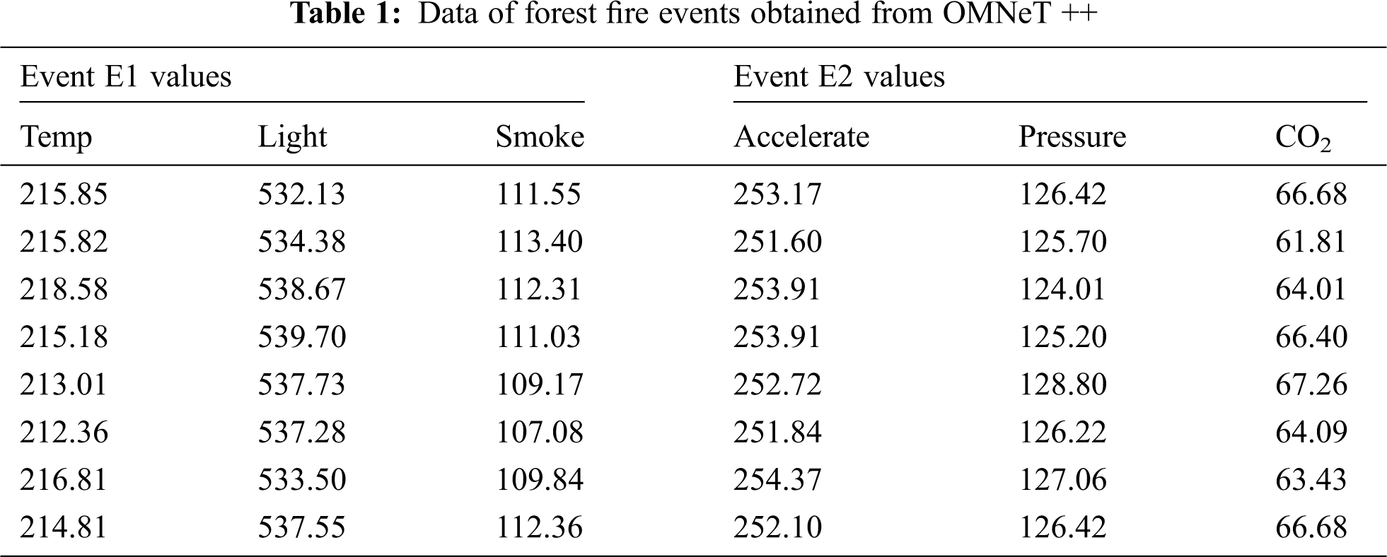
Each event attribute (variable) obtains the data values randomly from the multivariate normal distribution model that runs in the OMNeT++ simulator, as shown in Tab. 1, which contains 8 data packets for the forest fire events E1 and E2.

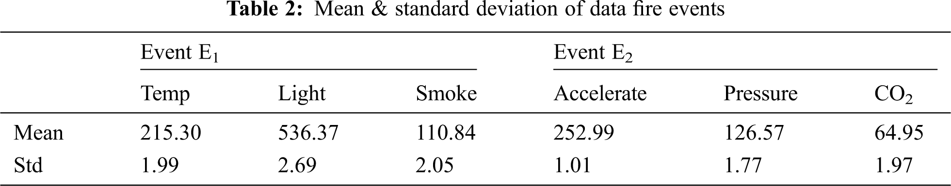
The mean and standard deviation for each variable are computed by MATLAB R2018b simulator.

•   Mean and Standard Deviation of Data Forest Fire Events Tab. 2

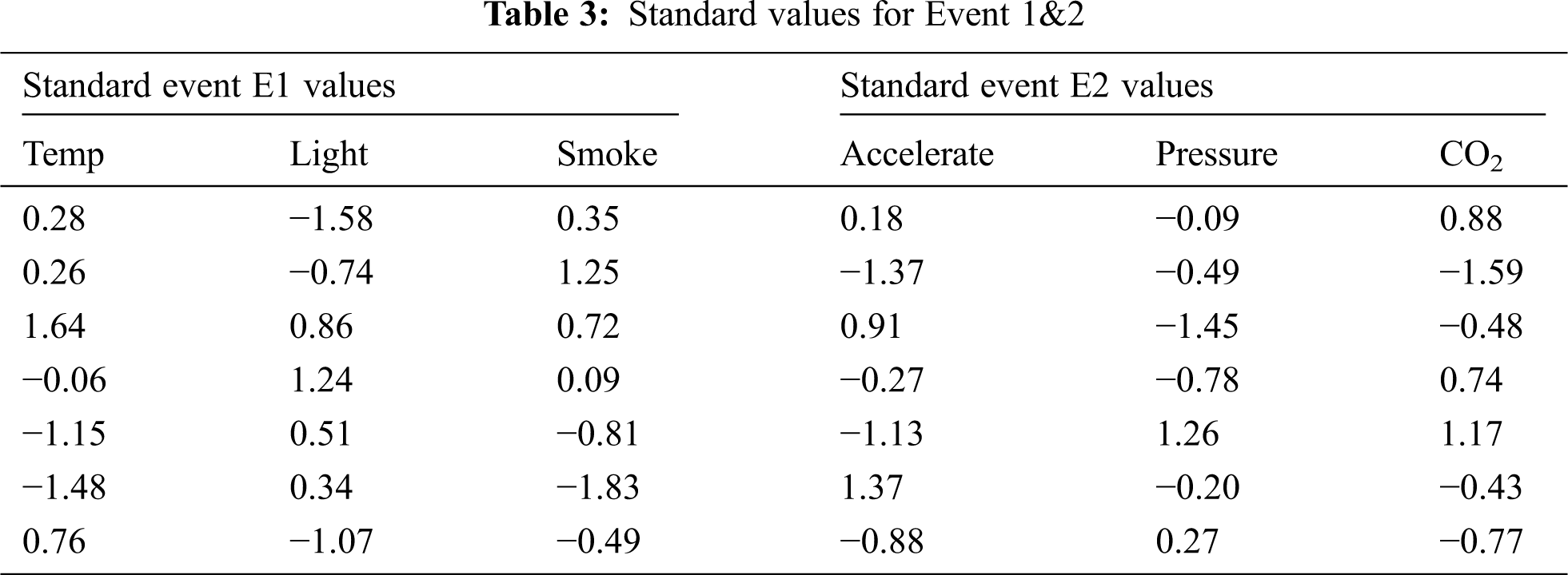
•   The standard values for each variable as in Tab. 3

•   The standard covariance for forest fire events as in Tab. 4

•   The standard correlation for forest fire events as in Tab. 5

•   The Eigenvalues for forest fire events as in Tab. 6

•   The Eigenvectors for forest fire events as in Tab. 7

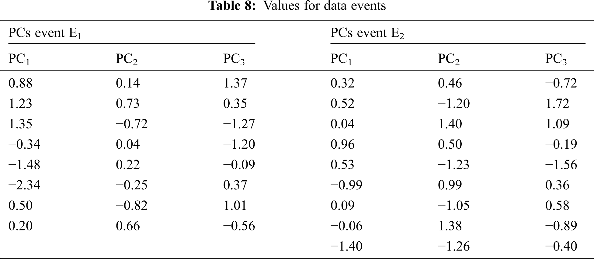
•   The PC values for both forest fire events as in Tab. 8

•   The variance for each PC value as in Tab. 9

It can be seen that PC1 is the first principal component for the forest fire event E1 due to the max variance, whereas PC2 is the first principal component for the forest fire event E2 due to the max variance. Thus, the PC1 data values represent the data variables’ values for E1, whereas the PC2 data values represent the data variables’ values for E2. It can be seen that the variance of PC values for each event equals the Eigenvalues for each event. Consequently, the examination results for PC1 data values for E1 and PC2 data values for E2 are given in Tab. 10.

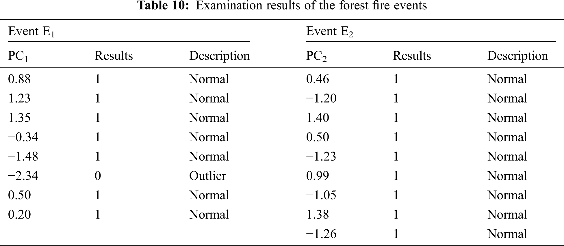
Tab. 10 shows that the sixth PC1 data value for the forest fire event E1 is −2.34, which does not fall within the required interval (−2, 2). Therefore, the sixth data value (212.36, 537.28, 107.08) for E1 is considered an outlier or anomalous value. On the other hand, there are no outlier values for event E2 because all PC data values that represent E2 attribute values fall within the required interval (−2, 2).

5  Simulation

OMNet++ is used to simulate the MOD scheme. In it, WSN is divided into clusters. Each cluster has CH and CMs. When an event is taken place, each node that senses event, sends data packet to the CH node. In the study, the coefficient times of the standard deviation (Stdcoff) determines the number of normal data values that should be aggregated. Also, bit error occurs in the transmission channel, changes the normal data values and affects the PC values so that they do not fall within the interval (StdCoff, StdCoff). Also, it is probable that the bit error changes the normal data values and does not affect the PC values. In the simulation, the transmission range, data packet size, metadata packet size and Ack packet size are 10 m, 128 bytes, 8 bytes and 4 bytes, respectively. The initial node energy is 5 * 103 Joules, whereby the node consumes 50 * 10−3 Joules to transmit or receive one bit. The data rate is 100 Mbps, propagation speed is 50 m/s, and the bit error rate is 0.00001 error/bit. However, some parameters are determined in each experiment, as shown in Tab. 11.

6  Results and Discussion

•   Simulation Results for MOD

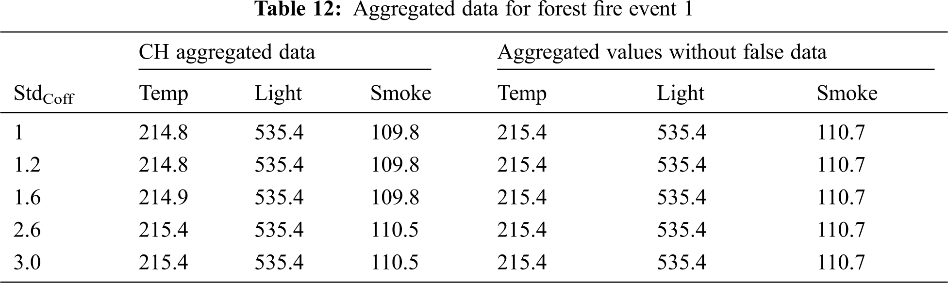
Tabs. 12 and 13 contain the aggregated data computed by the CH node and the aggregated values of the data sent by the CM nodes without any false data for both events. The tables show that there is a difference in the CH aggregated data when StdCoff is changed due to the increased number of normal data packets that are aggregated by the CH node. There is a bit error rate that occurs in the transmission channel, which changes the data events’ values. For instance, the number of normal data packets that can be aggregated by the CH node for event E1 when StdCoff equals 1, 1.6 and 2.6 are 4, 7 and 8. Therefore, the CH aggregated data packets for event E1 when StdCoff equals 1, 1.6 and 2.6 are (214.8, 535.4, 109.8), (214.9, 535.4, 109.8) and (215.4, 535.4, 110.5), respectively, as shown in Tab. 12.

On the other hand, the number of data packets transmitted by the CM nodes for event E1 when StdCoff equals 1, 1.6 and 2.6 is constant at 8 data packets, as shown in Tab. 13. Therefore, the aggregated data packet without any false data before transmission when StdCoff equals 1, 1.6 and 2.6 is (215.4, 535.4, 110.7). However, error in aggregation results is achieved, which is given by

Errorinaggregationresults=CHAggregatedData−NodesAggregatedDatawithoutfalse (16)

In this study, the event consists of a set of attributes. To compute each attribute’s accuracy, the following equation has been applied:

Attributei_Accuracy=1−Errorintheaggregationresults (17)

To compute the aggregated data accuracy, the average of the attributes’ accuracy has been found as given by

AggregatedDataAccuracy=∑i=1kAttributei_Accuracyk (18)

where k is the number of events that occur at same time within the cluster.

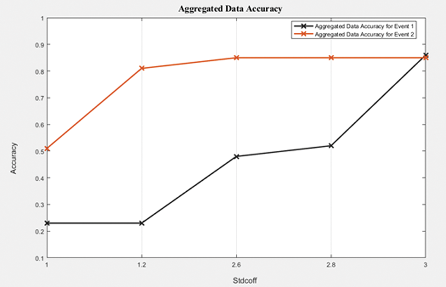
Figure 2: Aggregated data accuracy for forest fire events 1 and 2

Based on Fig. 2, it can be seen that when StdCoff value increased, the aggregated data accuracy for both events increased due to the increased number of PC1 and PC2 data values that fall within the required interval (−StdCoff, StdCoff), which represents the number of normal data packets that can be aggregated for both events. Also, the aggregated data accuracy for both events increased when StdCoff value increased due to the reduced error in the aggregation results.

•   Evaluation of MOD Algorithm

This section presents the evaluation of the MOD algorithm and compares it with the FTDA algorithm. Hence, it deals with the composite events by measuring the aggregated data accuracy for both using the same simulation parameters.

The measurement of the aggregated data accuracy for event E1 is achieved by computing the average of attributes’ accuracy when StdCoff changed. The evaluation of the MOD algorithm results in comparison with the FTDA algorithm is achieved by comparing the aggregated data accuracy for event E1 of the MOD algorithm with that of the FTDA algorithm.

•   FTDA-Aggregated Data for Event 1 by CH

•   FTDA-Aggregated Data for Event 1 without False Data

In Tab. 14, the CH aggregated data for each attribute are different when the percentage of false data is changed due to the increased number of normal data packets that were aggregated by the CH node and the impact of the bit error that occurred in the transmission channel, which changed the data values during transmission. In Tab. 15, the aggregated values for the data transmitted by CM nodes are the same when the percentage of false data is changed; this is because all CM nodes in the cluster obtained the same number of data packets which were generated by multivariate normal distribution in each experiment, and the bit error did not impact the sensed data before transmission occurred.

•   FTDA-Aggregated Data Accuracy

Tab. 16 contains the data accuracy for each attribute. The average of attributes’ accuracy has been calculated for when the percentage of false data changed. For instance, the average of the following attributes’ accuracy (0.11, 0.48, 42) is 0.34 when the percentage of false data equals 32%.

In the FTDA algorithm, when the percentage of false data was reduced, the aggregated data accuracy for the event increased. On the other hand, when StdCoff increased, the aggregated data accuracy for the event increased due to the reduced percentage of false data.

In another aspect, the aggregated data accuracy was evaluated when the StdCoff parameter was changed for the MOD algorithm in each experiment. The aggregated data computed by the CH node and the aggregated data sent by the active source nodes without false data for event 1 are shown in Tab. 17.

•   MOD Aggregated Data for Forest Fire Event 1 at Two Operation Cycles

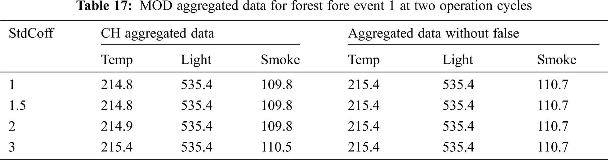
Tab. 17 illustrates the CH aggregated data for each event E1 attribute when StdCoff increased. The CH aggregated data for each attribute are different when StdCoff is changed due to the increased number of normal data packets that were aggregated by the CH node.

•   MOD Aggregated Data Accuracy for Forest Fire Event 1

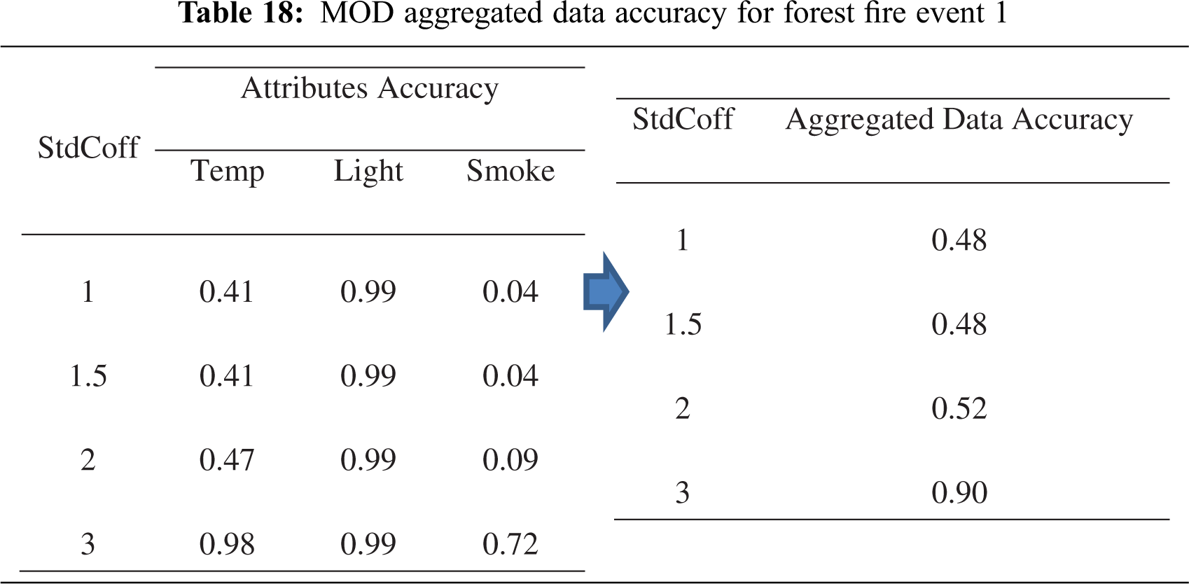
The measurement of the aggregated data accuracy for event E1 was achieved by computing the average of attributes’ accuracy when StdCoff changed. Tab. 18 shows the attribute accuracy and the aggregated data accuracy, which increased when StdCoff increased due to the increased number of PC1 data values and reduced error in the aggregation results.

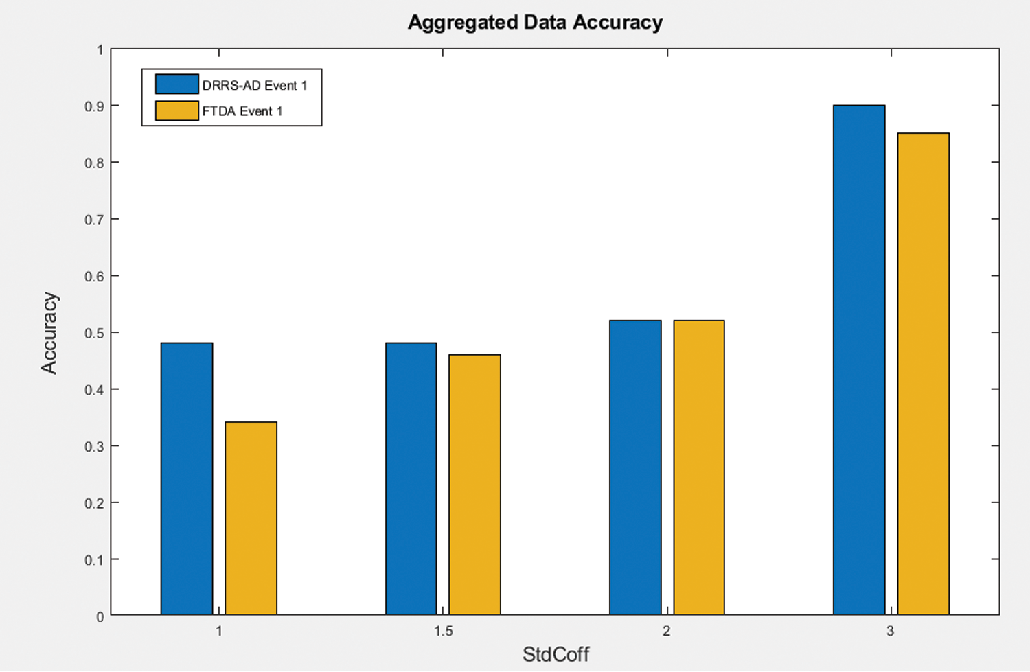
Figure 3: Aggregated data accuracy for MOD & FTDA algorithms

Fig. 3 displays the aggregated data accuracy for the MOD and FTDA algorithms. This figure illustrates that one event occurs within the cluster for both algorithms. It can be seen that the aggregated data accuracy increased when StdCoff increased for both algorithms due to the increased number of PC1 data values which fall within the required interval (−StdCoff, StdCoff) for the MOD algorithm and the decreased number of outlier data packets that were received by the CH node for the FTDA algorithm, respectively. Also, the aggregated data accuracy in the MOD algorithm was higher than in the FTDA algorithm when StdCoff increased from 1 to 3 for event E1. This is because the number of PC1 data values that do not fall within the required interval (−StdCoff, StdCoff), which represents the number of outlier data values of the MOD algorithm, is less than the number of outlier data packets that were received by the CH node under the FTDA algorithm. Consequently, the MOD algorithm conserved approximately 59.5% of aggregated data accuracy for event E1, compared with the FTDA algorithm’s 54.25%.

7  Conclusions

All CM nodes that have the event in their sensing range will detect the same event and produce redundant data. Part of these data may be incorrect due to redundancy. Thus, the CH node implements data aggregation to remove redundant data, but at the cost of the aggregated data accuracy, which is crucial in decision-making applications regarding forest fire occurrence. This research aimed to evaluate a multivariate outlier detection algorithm to conserve aggregated data accuracy. It was found that the aggregated data accuracy was conserved more by the MOD algorithm than by the FTDA algorithm, as the MOD algorithm conserved approximately 59.5% of aggregated data accuracy for event E1, compared to 54.25% for the FTDA algorithm.

Acknowledgement: The authors thank Alzaytoonah University of Jordan for their support.

Funding Statement: The authors received no specific funding for this study.

Conflicts of Interest: The authors declare that they have no conflicts of interest to report regarding the present study.

References

 1.  S. Khriji, G. Vinas Raventos, I. Kammoun and O. Kanoun, “Redundancy elimination for data aggregation in wireless sensor networks,” in 2018 15th Int. Multi-Conf. on Systems, Signals & Devices, Yasmine Hammamet, Tunisia, pp. 28–33, 2018. [Google Scholar]

 2.  D. E. Boubiche, S. Boubiche and Bilami, “Toward adaptive data aggregation protocols in wireless sensor networks,” in Proc. of Int. Conf. of Internet Things Cloud Computing, Cambridge United Kingdom, pp. 1–6, 2016. [Google Scholar]

 3.  S. Zhang, H. Chen, Q. Zhu and J. Jia, “A fuzzy-decision based approach for composite event detection in wireless sensor networks,” Scientific World Journal, vol. 2014, no. 5, pp. 1–20, 2014. [Google Scholar]

 4.  Y. Zhang, N. Meratnia and P. Havinga, “Outlier detection techniques for wireless sensor networks: A survey,” IEEE Communication, Surveys & Tutorials, vol. 12, no. 2, pp. 159–170, 2010. [Google Scholar]

 5.  A. A. A. Alkhatib, M. W. Elbes and E. M. Abu Maria, “Improving accuracy of wireless sensor networks localisation based on communication ranging,” IET Communications, vol. 14, no. 18, pp. 3184–3193, 2020. [Google Scholar]

 6.  S. Ozdemir and Y. Xiao, “FTDA: Outlier detection-based fault-tolerant data aggregation for wireless sensor networks,” Security and Communication Networks, vol. 6, no. 6, pp. 702–710, 2013. [Google Scholar]

 7.  K. Khedo, R. Doomun and S. Aucharuz, “READA: Redundancy elimination for accurate data aggregation in wireless sensor networks,” Wireless Sensor Network, vol. 2, no. 4, pp. 300–308, 2010. [Google Scholar]

 8.  T. Banerjee, B. Xie and D. P. Agrawal, “Fault tolerant multiple event detection in wireless sensor network,” Journal of Parallel Distributed Computing, vol. 68, no. 9, pp. 1222–1234, 2008. [Google Scholar]

 9.  G. Li, B. He, H. Huang and L. Tang, “Temporal data-driven sleep scheduling and spatial data-driven anomaly detection for clustered wireless sensor networks,” Sensors (Switzerland), vol. 16, no. 10, pp. 1–18, 2016. [Google Scholar]

10. L. Morissette and S. Chartier, “The k-means clustering technique: General considerations and implementation in mathematica,” Tutorials in Quantitative Methods for Psychology, vol. 9, no. 1, pp. 15–24, 2013. [Google Scholar]

11. J. Zhuang, Y. Pan and L. Chai, “Minimizing energy consumption with probabilistic distance models in wireless sensor networks,” in Proc. of IEEE INFOCOM, San Diego, CA, USA, 2010. [Google Scholar]

12. A. C. Rencher, “Random vectors and multivariate normal distribution,” in Multivariate Statistical Inference and Applications. New York: Wiley, pp. 32–67, 1997. [Google Scholar]

13. Y. L. Tong, “Multivariate normal distribution,” in The Multivariate Normal Distribution. Berlin, Germany: Springer Science & Business Media, pp. 1–19, 2012. [Google Scholar]

14. Ben Foley, “An introduction to variance, covariance & correlation,” Surveygizmo. (accessed Oct. 09, 20202018. [Online]. Available: https://www.surveygizmo.com/resources/blog/variance-covariance-correlation/. [Google Scholar]

15. P.-N. Tan and M. Steinbach, Introduction to Data Mining. Boston: Person Int, PEARSON Addison Wesley, 2006. [Google Scholar]

This work is licensed under a Creative Commons Attribution 4.0 International License, which permits unrestricted use, distribution, and reproduction in any medium, provided the original work is properly cited.