DOI:10.32604/iasc.2022.020362
| Intelligent Automation & Soft Computing DOI:10.32604/iasc.2022.020362 | |
| Article |
Machine Learning Empowered Software Defect Prediction System
1College of Engineering, Al Ain University, Abu Dhabi, 112612, UAE
2School of Computer Science, National College of Business Administration & Economics, Lahore, 54000, Pakistan
3Department of Computer Science, Virtual University of Pakistan, Lahore, 54000, Pakistan
4Riphah School of Computing & Innovation, Faculty of Computing, Riphah International University, Lahore Campus, Lahore, 54000, Pakistan
5Pattern Recognition and Machine Learning Lab, Department of Software, Gachon University, Seongnam, 13557, Korea
6School of Computer Science, Kean University, Union, NJ 07083, USA
7Department of Computer Science, College of Science and Technology, Wenzhou Kean University, 325060, China
*Corresponding Author: Muhammad Adnan Khan. Email: adnan@gachon.ac.kr
Received: 20 May 2021; Accepted: 21 June 2021
Abstract: Production of high-quality software at lower cost has always been the main concern of developers. However, due to exponential increases in size and complexity, the development of qualitative software with lower costs is almost impossible. This issue can be resolved by identifying defects at the early stages of the development lifecycle. As a significant amount of resources are consumed in testing activities, if only those software modules are shortlisted for testing that is identified as defective, then the overall cost of development can be reduced with the assurance of high quality. An artificial neural network is considered as one of the extensively used machine-learning techniques for predicting defect-prone software modules. In this paper, a cloud-based framework for real-time software-defect prediction is presented. In the proposed framework, empirical analysis is performed to compare the performance of four training algorithms of the back-propagation technique on software-defect prediction: Bayesian regularization (BR), Scaled Conjugate Gradient, Broyden–Fletcher–Goldfarb–Shanno Quasi-Newton, and Levenberg-Marquardt algorithms. The proposed framework also includes a fuzzy layer to identify the best training function based on performance. Publicly available cleaned versions of NASA datasets are used in this study. Various measures are used for performance evaluation including specificity, precision, recall, F-measure, an area under the receiver operating characteristic curve, accuracy, R2, and mean-square error. Two graphical user interface tools are developed in MatLab software to implement the proposed framework. The first tool is developed for comparing training functions as well as for extracting the results; the second tool is developed for the selection of the best training function using fuzzy logic. A BR training algorithm is selected by the fuzzy layer as it outperformed the others in most of the performance measures. The accuracy of the BR training function is also compared with other widely used machine-learning techniques, from which it was found that the BR performed better among all training functions.
Keywords: Software defect prediction; machine learning; artificial neural network
The development of high-quality software has always been the main concern of developers. In the modern era, it is almost impossible to provide qualitative software within a limited time and at a lower cost. This is due to the exponential increase in the size and complexity of required software [1–3]. To achieve bug-free software, a thorough and well-managed quality-assurance process is needed. To ensure the high quality of software, each module should be properly tested before integration. Thus, if the development team could know which software modules were defective in advance, then a significant amount of time would be saved by focusing on those modules in which defects were most likely to occur [4,5]. With this approach, the development of high-quality software within a limited time and at a lower cost can be possible [6]. The task of identifying the defective modules before testing is known as a software-defect prediction. The detection of defective modules by using machine-learning techniques has been the object of wide focus by researchers in the past two decades [7]. Artificial neural networks (ANNs) are among the most widely used supervised machine-learning techniques to detect defective modules at the early stages of software development [8]. The techniques that are among supervised machine-learning approaches use pre-labeled data (also known as training data) to train the classification model. During the training process, the particular model makes the classification rules that are further used to classify the test data (unseen data) during the classification process [9–15]. In this paper, a cloud-based framework is proposed to predict defect-prone software modules in real-time environments. The proposed framework contributes by analyzing and comparing the performance of four variants of back-propagation training techniques during the detection of defective modules. The training techniques include Bayesian regularization (BR), scaled conjugate gradient (SCG), BFGS quasi-Newton (QN), and Levenberg-Marquardt (LM) techniques. A fuzzy layer is also included in the framework for the selection of the best training function by analyzing the results of all four training algorithms based on fuzzy rules. Cleaned versions of NASA datasets were used in the experiments, including KC1, KC3, JM1, CM1, MW1, PC1, PC2, PC3, PC4, PC5, MC1, and MC2. Various measures were used for performance evaluation, including specificity, recall, precision, F-measure, accuracy, an area under the curve (AUC), R2, and mean-square error (MSE). The fuzzy logic is implemented to select the best training function. The BR training function is selected by fuzzy layer as it performed well in most of the performance measures compared to other training algorithms. The accuracy of the BR training function in each dataset was also compared with other widely used machine-learning algorithms, and it was observed that BR outperformed all other techniques.
Various studies have contributed to achieving high accuracy in software-defect prediction as well as in other classification problems by using machine-learning techniques, several of which are discussed here. In [16], the researchers developed a GUI tool in MatLab and used a BR training algorithm to predict software defects. The software cost is reduced by limiting the error rate. The accuracy of BR was analyzed compared to the LM technique. The results reflected that BR outperformed the LM technique. Researchers in [17] performed an empirical comparison of a support vector machine (SVM) and an ANN on software-defect predictive capability. Seven datasets were selected from the NASA PROMISE repository for the experiments. The performance was measured and analyzed by using specificity, accuracy, and recall. Results showed that the SVM outperformed the ANN in recall score. Researchers in [18] presented a Matlab-based GUI tool that used the object-oriented metrics from Chidamber and Kemerer (CK) for software-defect prediction. The aforementioned datasets from the NASA PROMISE repository were used for the experiments. The accuracy of the LM training technique was compared with the ANN-based on a polynomial function, and the results indicated that the proposed model showed higher accuracy. In [19], researchers presented a framework by using a modified and new artificial bee colony technique and an ANN to extract the best weights. Five datasets from the publicly available library were used for the experiments, and the results of the proposed framework reflected higher performance compared with other techniques. In [20], researchers presented a Matlab-based GUI tool for the classification of diabetic patients. The proposed tool can detect the disease without the presence of a doctor and also can help doctors obtain records of diabetic patients within seconds so that the disease can be diagnosed in real-time. Researchers in [21] introduced a hybrid genetic algorithm- (HGA-) based approach to reduce the number of features. For the classification of software defects, they used a deep neural network and the PROMISE dataset repository for experiments. Results showed that the proposed approach delivered good results when compared with other software-defect-prediction techniques. In [22], researchers proposed a hybrid ANN (HANN) with a quantum particle swarm optimization (QPSO) technique for software-defect prediction. An ANN was used for predicting the defective and non-defective modules, whereas QPSO was used for dimensionality reduction. The experimental results reflected that the proposed approach outperformed many conventional and modern techniques. The researchers in [23] used three cost-sensitive boosting techniques to improve the performance of ANNs on software-defect prediction. The first technique is based on a threshold moving strategy, and the other two techniques work by updating the weights. The performance of the techniques used was evaluated on four NASA datasets. Results reflected that the technique that used a threshold moving average is better among the three techniques used. In [24], researchers proposed a defect-prediction framework by using a convolutional neural network (CNN). The proposed framework leveraged deep learning to extract features based on program abstract syntax trees (ASTs). The extracted token vectors are encoded into numeric vectors and then given as input to the CNN for learning, and finally, the learned features and traditional hand-crafted features are combined. The proposed technique was evaluated on seven open-source projects by using F-measure as the accuracy measure. Results showed that the proposed technique outperformed other modern methods. The researchers in [25] proposed a conventional radial basis function-based technique integrated with a novel adaptive dimensional biogeography-based optimization model for software-defect predication. Five NASA datasets from the PROMISE repository were used for experimental analysis, the results of which showed that the proposed technique is effective compared to earlier proposed models.
In this paper, an intelligent real-time, cloud-based software-defect-prediction system is proposed. The performance of four variants of a back-propagation training algorithm on the prediction of defect-prone software modules, followed by the selection of a highly effective training algorithm by using a fuzzy layer, is analyzed and compared using the proposed framework.
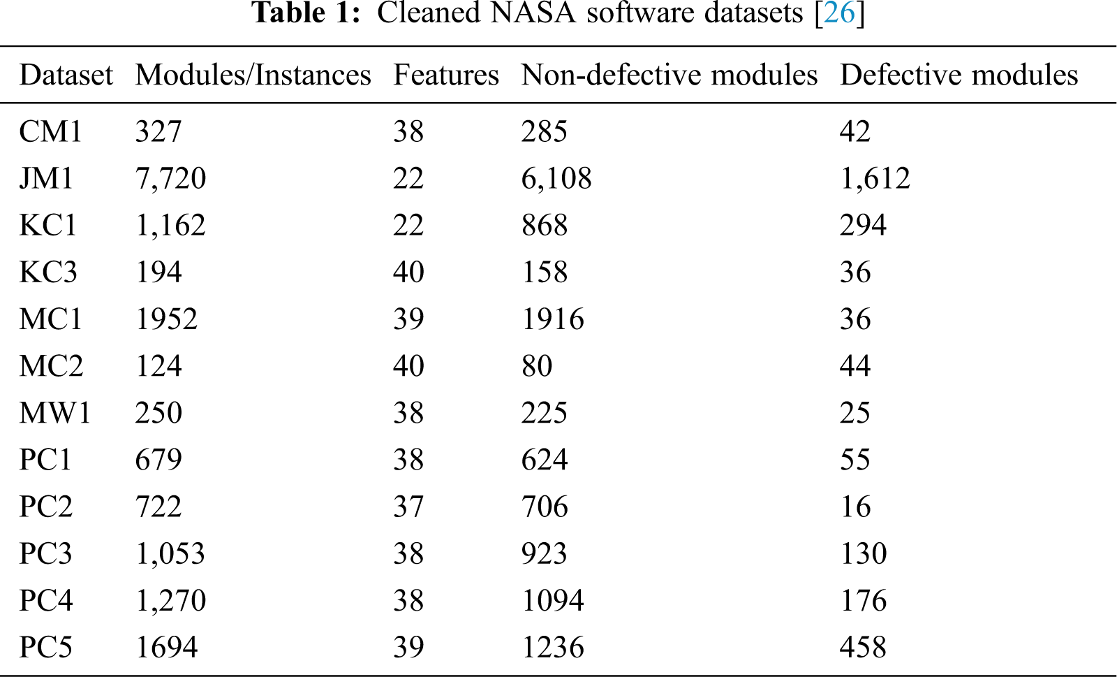
The proposed framework consists of two phases: training and testing as shown in Fig. 1. The training phase is initiated with the selection of datasets. Twelve cleaned NASA datasets were used for the comparison: KC1, KC3, JM1, CM1, MW1, PC1, PC2, PC3, PC4, PC5, MC1, and MC2 (see Tab. 1). Two versions of NASA's clean datasets, i.e., DS′ and DS″, were provided by [26]. DS′ includes inconsistent and duplicate values, whereas DS″ does not include any such instances. These datasets were initially available from the site referenced in [27] but were removed. In the present work, DS″ datasets that are currently available from the site referenced in [28] were used. DS″ datasets were already discussed and used in [29–31]. Each dataset contains many independent features and only one dependent feature, which is also called the target class. The dependent feature is predicted based on independent features. The attribute “target class” contains a nominal value of Boolean type, either “Y” or “N.” The Boolean value of Y reflects that the particular module is defective, whereas the value of N means that the module is non-defective. The used datasets include various independent features, such as cyclomatic density, cyclomatic complexity, effort, line of code, decision density, decision count, and design density, etc. All these measures collectively help to predict the target class. During the experiments, the values of the target class are included in the datasets so that the output results of the ANN models can be compared with the values of the target class for performance analysis. After the selection of an appropriate dataset, the first layer of the training phase deals with pre-processing activities. First, the missing values are removed, followed by the normalization process, in which outliers are removed by keeping the values of all the attributes within a certain limit (0–1). The third activity in this layer deals with the process of splitting the dataset into training and test data. In this research, 70% of the data were used for training and 30% for testing. The second layer deals with the classification process by using four variants of a back-propagation technique: BR, SCG, BFGS-QN, and LM techniques. Performance was analyzed in testing using various measures, including precision, specificity, F-measure, recall, AUC, MSE, accuracy, and R2. For simulation and performance comparison, a GUI tool was developed in MatLab (version r2018) [32]. A fuzzy layer was also included in the proposed framework to select the best training algorithm based on performance in all of the accuracy measures used. The fuzzy layer receives the results of four training algorithms and stores the classification model in a cloud with the one training algorithm that outperformed the others. A development team can use the model from the cloud to classify the datasets as a real-time project and thereby reduce the testing cost.
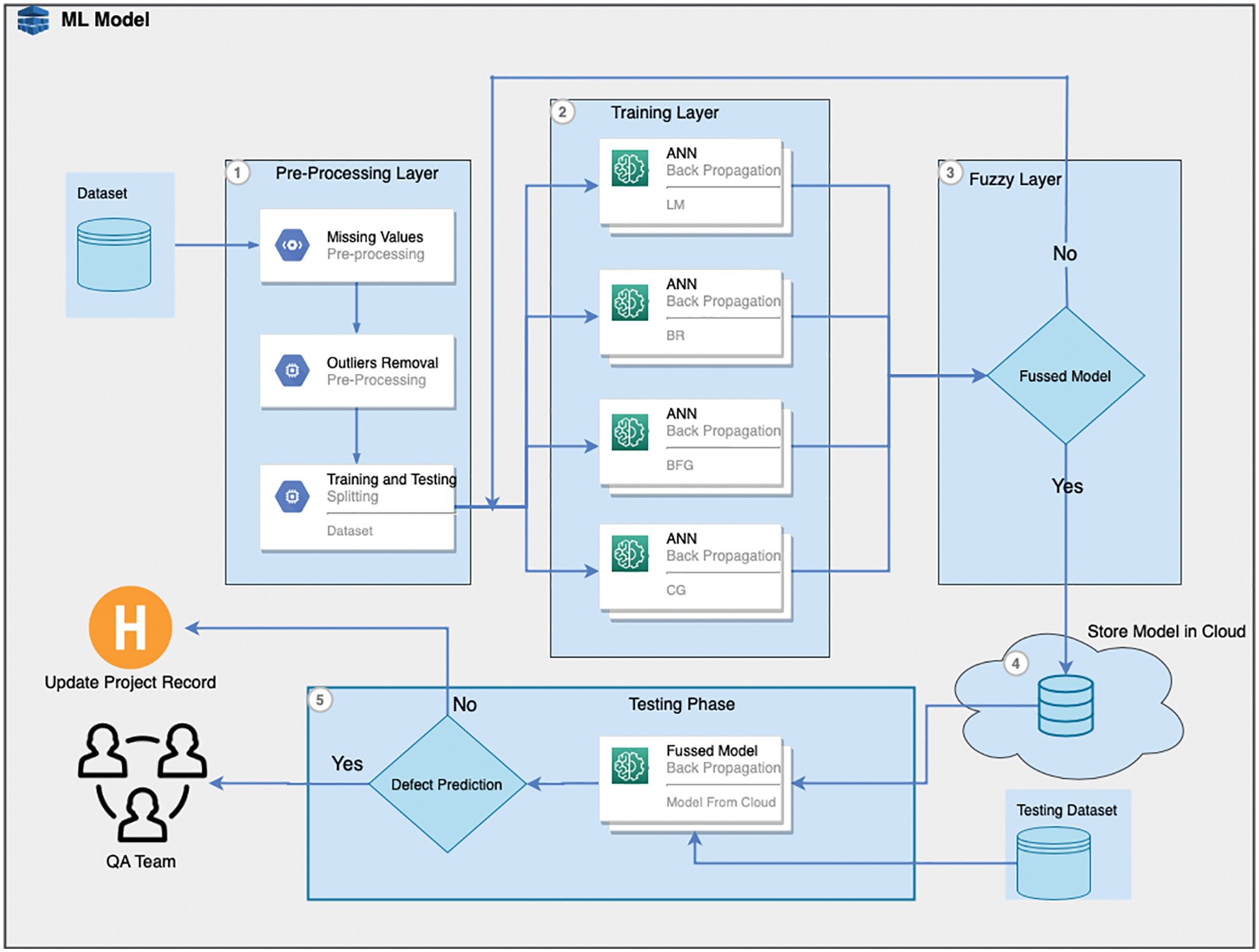
Figure 1: Cloud based software defect prediction framework
An ANN is an interconnected set of units called neurons. It processes the information by following a computational model. The structure of a basic ANN is shown in Fig. 2.
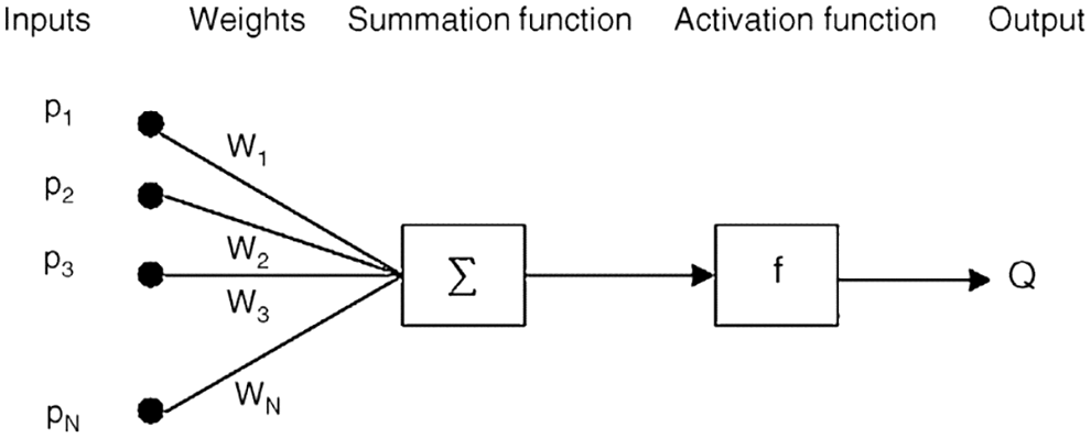
Figure 2: Neural network architecture
The first layer of an ANN is called the input layer, in which the number of neurons is equal to the number of input values, followed by the computation methodology, and finally, the output layer, in which the number of neurons is reflected by the number of output classes. An ANN can learn rapidly from the experiences of complex nonlinear problems [33]. An ANN model has been reported to be an effective classifier for detecting software defects at the early stages of the software development life cycle. During the feed-forward process in an ANN, the layers receive the inputs only from the previous layer. Each unit in one layer relates to all the units in the next layer. All these connections contain different weights and strengths. The weights of the connections reflect the potential knowledge of the network. When a feed-forward neural network (FFNN) acts as a classifier, then usually there is no feedback between the layers. The information processing of the network includes data entry from the input units, passing through the hidden layers until reaching the output layer towards one direction (forward); this is why it is called an FFNN [34]. A BP algorithm is one of the highly adopted learning methods for an ANN and belongs to the supervised class of training algorithms that attempt to gradually reduce the error of a NN [35]. The training data are estimated iteratively through the input layer to predict the correct output.
A multi-layer perceptron uses at least one hidden layer in addition to input and output layers. Various steps are involved in a BP algorithm, including initialization of weight, a FF process, and a back-propagation process based on errors and updating weights and biases.
Each of the neurons in the hidden layer has an activation function like f(a)=Sigmoid(a). The sigmoid function for input and the hidden layer of the ANN used can be written as
The input derived from the output layer is
The activation function of the output layer is expressed as
The BP error is represented by Eq. (5), where τt and φt represent the desired output and estimated output, respectively. In the following equation, the rate of change in weight for the output and that in the layer are written as
respectively. After applying the chain rule method, Eq. (6) can be re-stated as
By substituting for the values in Eq. (7), the value of the weight change can be obtained as follows:
where
Applying the chain rule for updating the weights between input and hidden layers gives
where ε represents a constant,
After simplification, the above equations can be re-stated as
where
Eq. (10) is used for updating the weights between hidden layers and output:
The weights between the hidden and input layers are updated using Eq. (11).
The BP process consists of two stages: forward and backward [35]. In this study, the performance of four learning functions of the BP technique is compared, namely the BR, SCG, BFGS QN, and LM techniques. The LM technique works based on a Hessian-based technique. The Hessian-based techniques are mostly used with NNs to make them learn with more appropriate features during complicated mapping. The LM method is also known as curve fitting because it combines gradient descent and Gauss-Newton (GN) techniques. It works as follows: If the parameter is far from its optimal value, this technique then acts as a gradient descent algorithm; if the parameter is close to its best value, then this technique acts like a GN algorithm [36]. BR is also known as one of the widely used learning techniques in BP processes. The optimization process in a BR learning technique is similar to the learning technique of the LM method as it tunes the weights, minimizes errors, and finally extracts the best combination so that the ANN can perform better [37,38]. The SCG technique uses a mechanism called step-size scaling that decreases the time used inline searching in each learning iteration [39]. The BFGS QN method uses the QN technique to decrease the sequence of error functions associated with a growing network [40]. A GUI was developed using MatLab r2018a for comparison and simulation. This tool facilitates the development and optimization of the ANN. Parameters available in the GUI tool include the selection of a dataset from a dropdown list as well as the selection of percentages of training, testing, and validation data, along with epoch size and the number of neurons. Moreover, the option to select the training function is also available for quick simulation instead of writing code. After extracting the results using four variants of the BP technique, fuzzy logic is used to select the best training function. Results from four training functions comprise the input of the fuzzy layer, and the output is the single best training function. The trained classification model using the particular training function is stored in the cloud and is extracted further to focus on the real-time software-defect dataset for bug prediction.
The results of empirical comparisons are presented here. Results of all datasets are extracted by each of the following training functions: LM, BR, BFG, and CG. An FFNN with a single hidden layer is used in the experiments. The hidden layer consisted of 10 neurons. To avoid random results, the model was executed 20 times, and the highest results were recorded. The performance of NN models is generally evaluated using statistical measures like R2 and MSE as well as measures computed from a confusion matrix, e.g., specificity, precision, recall, F-measure, accuracy, and AUC [39–41].
Performance measures extracted from the confusion matrix are listed below.
Results on different datasets are presented in Tabs. 2–13.
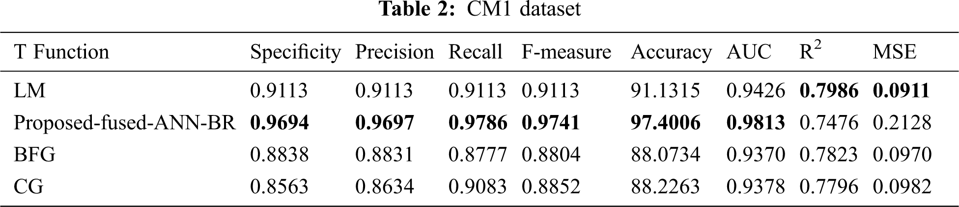
Tab. 2 shows the results of the CM1 dataset. It can be seen that the proposed fused-ANN-BR outperformed other training algorithms in Accuracy with a score of 97.4006.
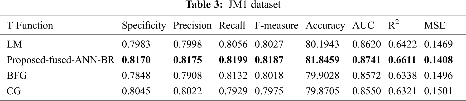
Tab. 3 shows the results for the JM1 dataset. The proposed fused-ANN-BR technique outperformed all other techniques in Accuracy with a score of 81.8459.
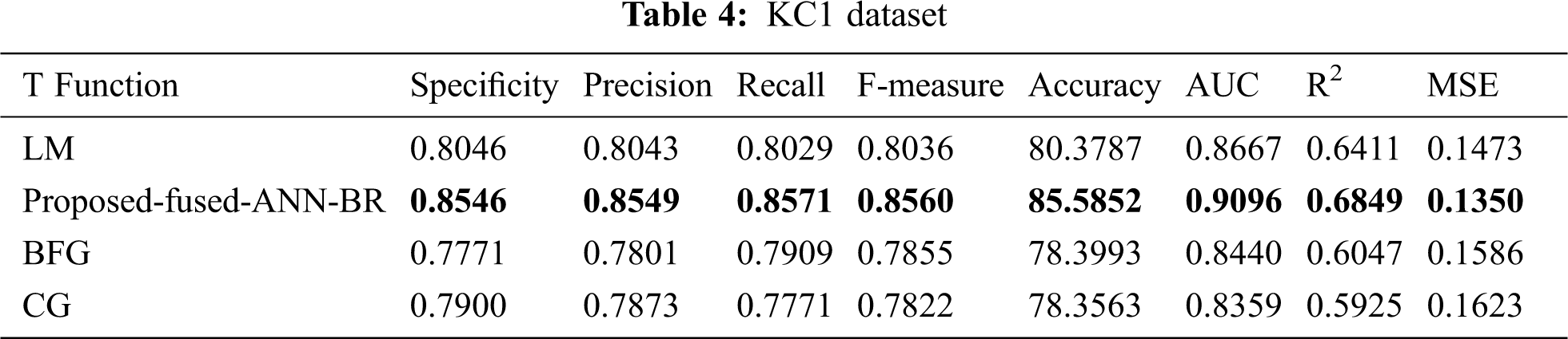
Tab. 4 shows the results for the KC1 dataset. The proposed Fused-ANN-BR technique outperformed all other techniques in Accuracy with a score of 85.5852.
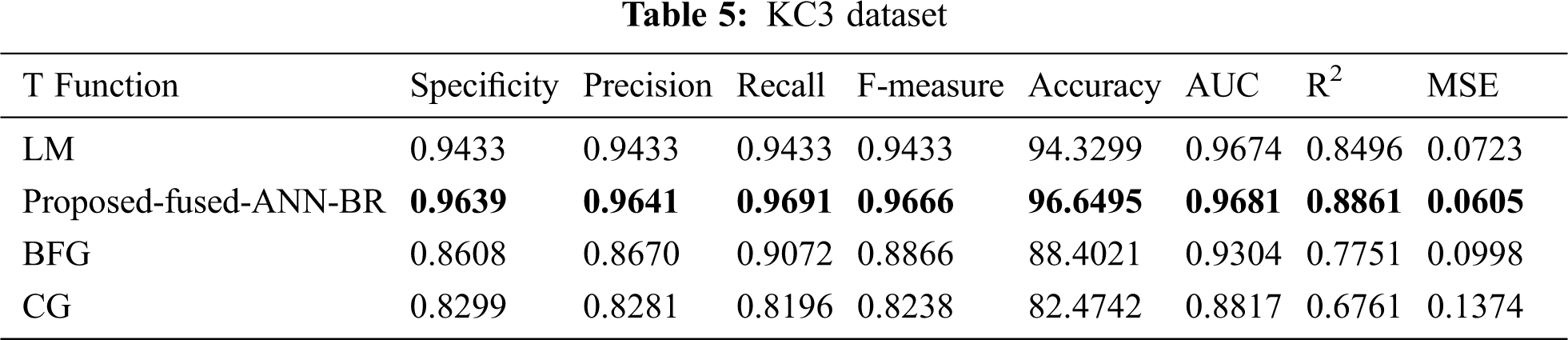
Tab. 5 shows the results for the KC3 dataset. It can be seen that the proposed fused-ANN-BR technique performed better in Accuracy with a score of 96.6495.
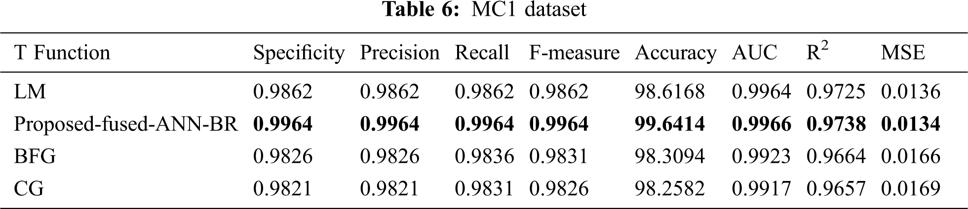
Tab. 6 shows the results for the MC1 dataset. The proposed fused-ANN-BR technique outperformed all other techniques in Accuracy with a score of 99.6414.
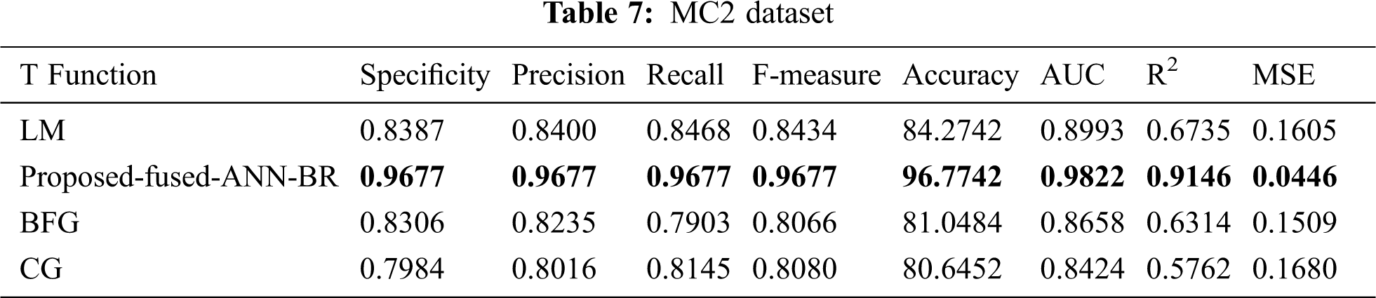
Tab. 7 shows the results for the MC2 dataset. The proposed fused-ANN-BR technique performed better than all other techniques in Accuracy and achieved a score of 96.7742.
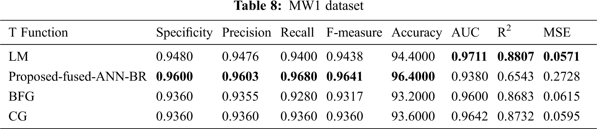
Tab. 8 shows the results for the MW1 dataset. The proposed fused-ANN-BR technique performed better than all other techniques in Accuracy with a score of 96.4000.
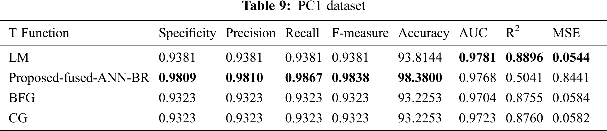
Tab. 9 shows the results for the PC1 dataset. The proposed fused-ANN-BR technique performed better than all other techniques in Accuracy with a score of 98.3800.
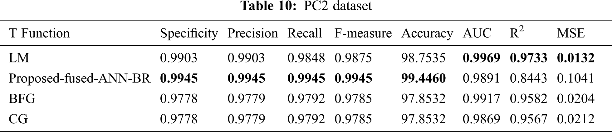
Tab. 10 shows the results for the PC2 dataset. The proposed fused-ANN-BR technique performed better than all other techniques in Accuracy with a score of 99.4460.
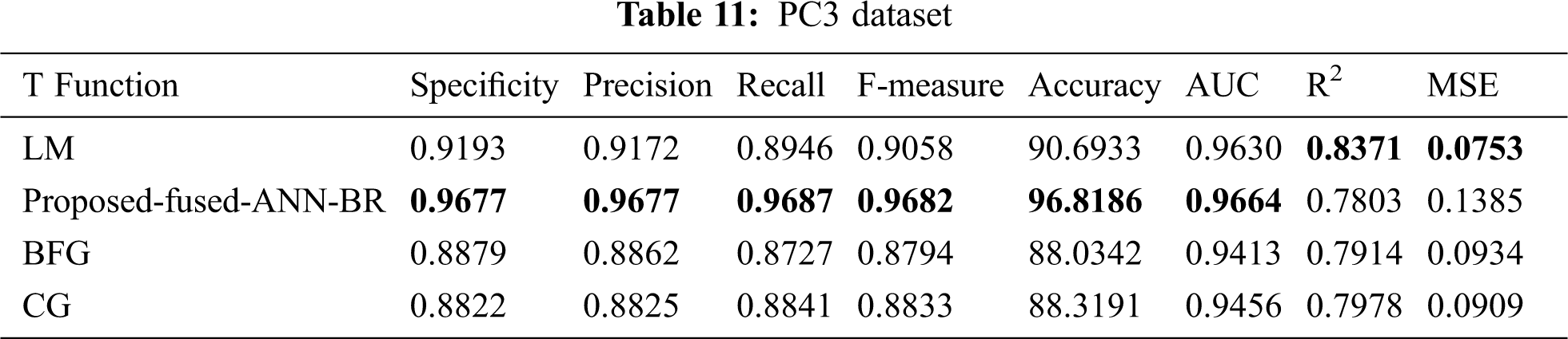
Tab. 11 shows the results for the PC3 dataset. The proposed fused-ANN-BR technique performed better than all other techniques in Accuracy with a score of 96.8186.
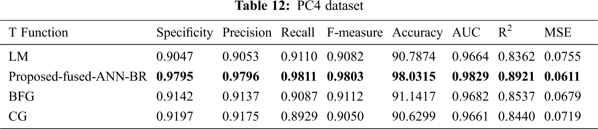
Tab. 12 shows the results for the PC4 dataset. The proposed fused-ANN-BR technique performed better than all other techniques in Accuracy with a score of 98.0315.
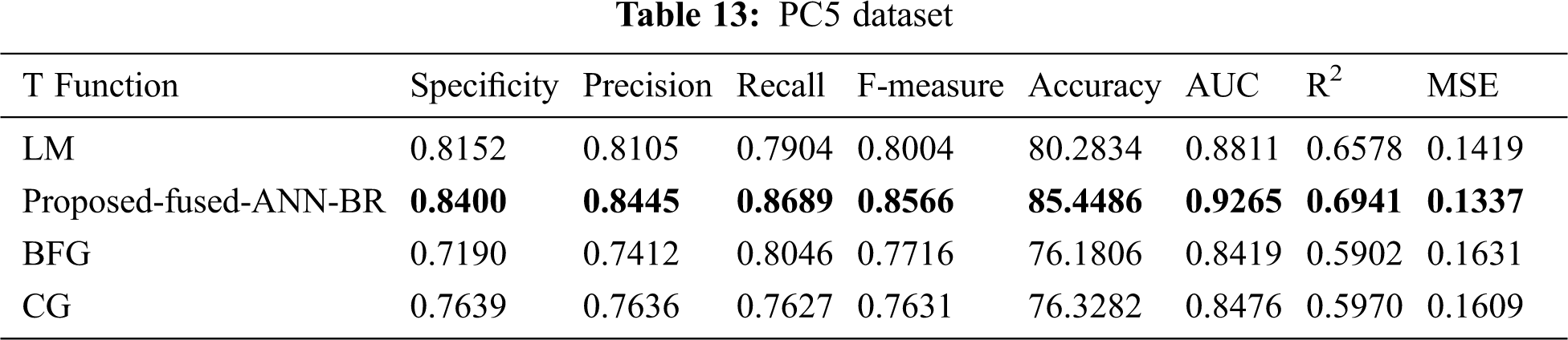
Tab. 13 shows the results for the PC5 dataset. The proposed fused-ANN-BR technique performed better than all other techniques in Accuracy with a score of 85.4486.
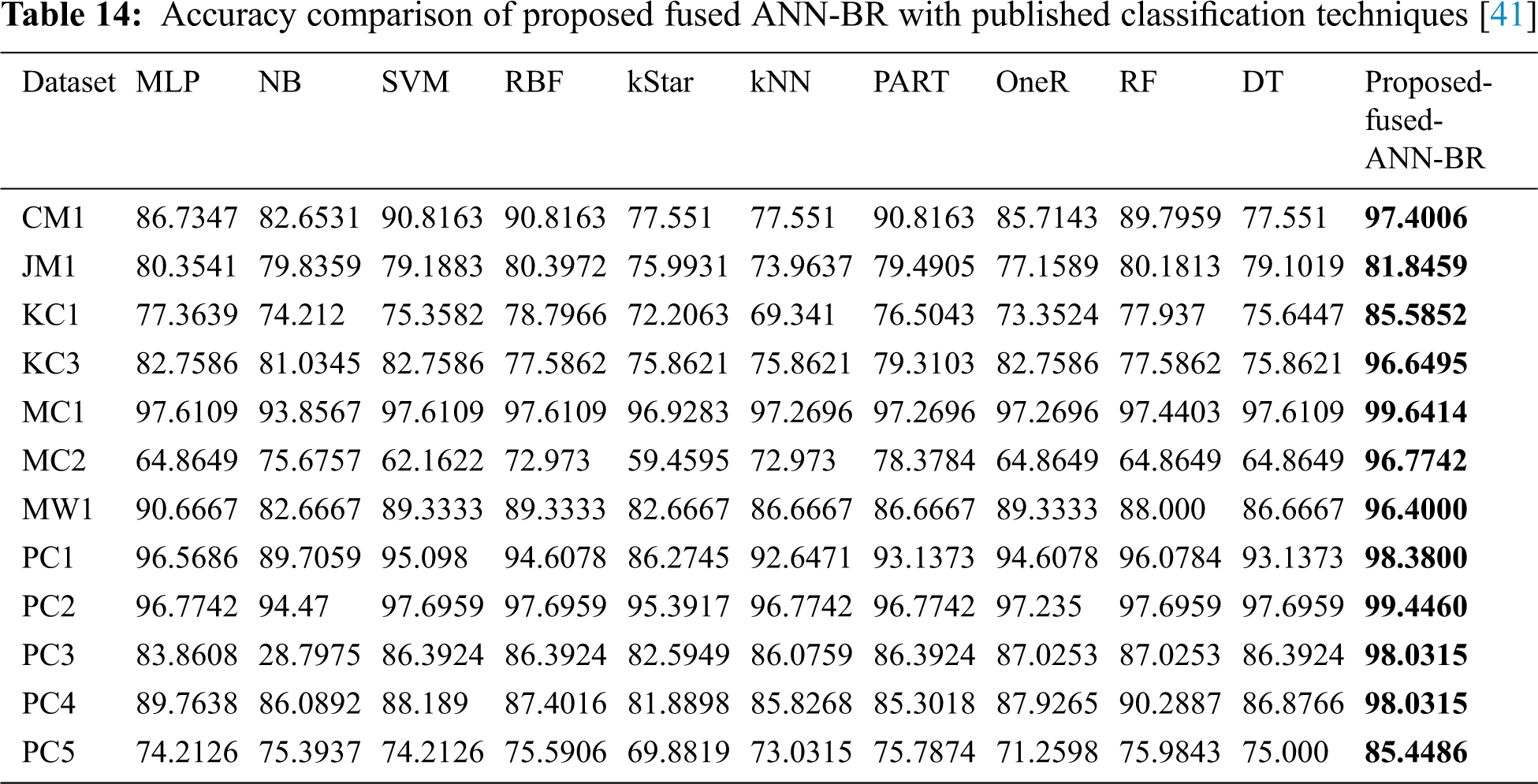
It can be seen from Tab. 14 the overall results that the fused-ANN-BR performed better with FFNN, but a lower MSE was achieved in several of the datasets used with the LM algorithm. The proposed fused-ANN-BR performed better on the CM1 and PC3 datasets in specificity, precision, recall, F-measure, accuracy, and AUC, but the LM technique performed better in R2 and MSE. Results on the JM1, KC1, KC3, MC1, MC2, PC4 and PC5 datasets reflect the higher performance of the proposed fused-ANN-BR algorithm in all measures. On the MW1, PC1, and PC2 datasets, BR outperformed the others in specificity, precision, recall, F-measure, and accuracy, but the LM technique outperformed the others in AUC, R2, and MSE. It has also been noted that BFG and CG could not perform better in any of the performance measures used. The fuzzy layer used in the model after comparison selected BR due to its high performance in most of the performance measures. A comparative analysis of the results obtained from the proposed fused-ANN-BR was also performed with those obtained by other widely used classification techniques from [41] that also used the same cleaned versions of the aforementioned datasets.
Four variants of back-propagation training algorithms used in software-defect prediction were compared on five publicly available cleaned NASA datasets, followed by a selection of the best algorithm by use of a fuzzy layer. The training algorithms compared were LM, BR, SCG, and BFGS-QN. To facilitate experiments, a GUI tool was developed in the MatLab environment to construct and tune the ANN models. Performance was evaluated by using the following measures: specificity, precision, recall, F-measure, accuracy, AUC, R2, and MSE. The fuzzy layer selected the BR algorithm as best performing as it performed better in most of the accuracy measures. However, a lower MSE value was achieved in some datasets using the LM technique. It is also noted that the BFG and SCG techniques did not show any significantly high performance in any of the accuracy measures used. Finally, the accuracy of the proposed fused-ANN-BR technique on each dataset was compared with other well-known machine-learning techniques, and it was found that BR performed better than all other techniques.
Acknowledgement: We thank our families and colleagues who provided us with moral support.
Funding Statement: No funding was received for this research.
Conflicts of Interest: The authors declare that they have no conflicts of interest to report regarding the present study.
1. S. Huda, S. Alyahya, M. Mohsin Ali, S. Ahmad, J. Abawajy et al., “A framework for software defect prediction and metric selection,” IEEE Access, vol. 6, pp. 2844–2858, 2017. [Google Scholar]
2. E. Erturk and E. A. Sezer, “A comparison of some soft computing methods for software fault prediction,” Expert Systems with Applications, vol. 42, no. 4, pp. 1872–1879, 2015. [Google Scholar]
3. R. Malhotra, “Comparative analysis of statistical and machine learning methods for predicting faulty modules,” Applied Soft Computing Journal, vol. 21, pp. 286–297, 2014. [Google Scholar]
4. I. H. Laradji, M. Alshayeb and L. Ghouti, “Software defect prediction using ensemble learning on selected features,” Information and Software Technology, vol. 58, pp. 388–402, 2015. [Google Scholar]
5. D. Tomar and S. Agarwal, “Prediction of defective software modules using class imbalance learning,” Applied Computational Intelligence and Soft Computing, vol. 2016, pp. 1–12, 2016. [Google Scholar]
6. D. Rodríguez, R. Ruiz, J. C. Riquelme and J. S. A. Ruiz, “Searching for rules to detect defective modules: A subgroup discovery approach,” Information Sciences, vol. 191, pp. 14–30, 2012. [Google Scholar]
7. H. A. Al-Jamimi and L. Ghouti, “Efficient prediction of software fault proneness modules using support vector machines and probabilistic neural networks,” in Malaysian Conference in Software Engineering, Johor Bahru, Malaysia, pp. 251–256, 2011. [Google Scholar]
8. O. I. Abiodun, A. Jantan, A. E. Omolara, K. V. Dada, N. A. E. Mohamed et al., “State-of-the-art in artificial neural network applications: A survey,” Heliyon, vol. 4, no. 11, pp. 938–945, 2018. [Google Scholar]
9. M. Ahmad, S. Aftab, M. S. Bashir, N. Hameed, I. Ali et al., “Svm optimization for sentiment analysis,” International Journal of Advanced Computer Science and Applications, vol. 9, no. 4, pp. 393–398, 2018. [Google Scholar]
10. M. Ahmad, S. Aftab, M. S. Bashir and N. Hameed, “Sentiment analysis using svm: A systematic literature review,” International Journal of Advanced Computer Science and Applications, vol. 9, no. 2, pp. 182–188, 2018. [Google Scholar]
11. S. Aftab, M. Ahmad, N. Hameed, M. S. Bashir, I. Ali et al., “Rainfall prediction using data mining techniques: A systematic literature review,” International Journal of Advanced Computer Science and Applications, vol. 9, no. 5, pp. 143–150, 2018. [Google Scholar]
12. M. Ahmad, S. Aftab, S. Muhammad and S. Ahmad, “Machine learning techniques for sentiment analysis: A review,” International Journal of Multidisciplinary Sciences and Engineering, vol. 8, no. 3, pp. 27–32, 2017. [Google Scholar]
13. S. Aftab, M. Ahmad, N. Hameed, M. S. Bashir, I. Ali et al., “Rainfall prediction in lahore city using data mining techniques,” International Journal of Advanced Computer Science and Applications, vol. 9, no. 4, pp. 254–260, 2018. [Google Scholar]
14. M. Ahmad and S. Aftab, “Analyzing the performance of svm for polarity detection with different datasets,” International Journal of Modern Education and Computer Science, vol. 9, no. 10, pp. 29–36, 2017. [Google Scholar]
15. M. Ahmad, S. Aftab and I. Ali, “Sentiment analysis of tweets using svm,” International Journal of Computer Applications, vol. 177, no. 5, pp. 25–29, 2017. [Google Scholar]
16. R. Mahajan, S. K. Gupta and R. K. Bedi, “Design of software fault prediction model using br technique,” Procedia Computer Science, vol. 46, no. Icict 2014, pp. 849–858, 2015. [Google Scholar]
17. I. Arora and A. Saha, “Software defect prediction: A comparison between artificial neural network and support vector machine,” Advances in Intelligent Systems and Computing, vol. 562, pp. 51–61, 2018. [Google Scholar]
18. M. Singh and D. Singh Salaria, “Software defect prediction tool based on neural network,” International Journal of Computer Applications, vol. 70, no. 22, pp. 22–28, 2013. [Google Scholar]
19. Ö. F. Arar and K. Ayan, “Software defect prediction using cost-sensitive neural network,” Applied Soft Computing, vol. 33, pp. 263–277, 2015. [Google Scholar]
20. S. Joshi and M. Borse, “Detection and prediction of diabetes mellitus using back-propagation neural network,” in Proc. Int. Conf. on Micro-Electronics and Telecommunication Engineering, Ghaziabad, India, pp. 110–113, 2016. [Google Scholar]
21. C. Manjula and L. Florence, “Deep neural network based hybrid approach for software defect prediction using software metrics,” Cluster Computing, vol. 22, pp. 9847–9863, 2019. [Google Scholar]
22. C. Jin and S. W. Jin, “Prediction approach of software fault-proneness based on hybrid artificial neural network and quantum particle swarm optimization,” Applied Soft Computing, vol. 35, pp. 717–725, 2015. [Google Scholar]
23. J. Zheng, “Cost-sensitive boosting neural networks for software defect prediction,” Expert Systems with Applications, vol. 37, no. 6, pp. 4537–4543, 2010. [Google Scholar]
24. J. Li, P. He, J. Zhu and M. R. Lyu, “Software defect prediction via convolutional neural network,” in IEEE Int. Conf. on Software Quality, Reliability and Security, Prague, Czech Republic, pp. 318–328, 2017. [Google Scholar]
25. P. Kumudha and R. Venkatesan, “Cost-sensitive radial basis function neural network classifier for software defect prediction,” Scientific World Journal, vol. 2016, pp. 1–20. 2016. [Google Scholar]
26. M. Shepperd, Q. Song, Z. Sun and C. Mair, “Data quality: Some comments on the nasa software defect datasets,” IEEE Transactions on Software Engineering, vol. 39, no. 9, pp. 1208–1215, 2013. [Google Scholar]
27. “NASA – software defect datasets” Online. Available: https://nasasoftwaredefectdatasets.wikispaces.com. Accessed: 01-April- 2019. [Google Scholar]
28. “NASA defect dataset.” Online. Available: https://github.com/klainfo/NASADefectDataset. Accessed: 01-April- 2019. [Google Scholar]
29. B. Ghotra, S. McIntosh and A. E. Hassan, “Revisiting the impact of classification techniques on the performance of defect prediction models,” in 37th IEEE Int. Conf. on Software Engineering, Florence, Italy, pp. 789–800, 2015. [Google Scholar]
30. G. Czibula, Z. Marian and I. G. Czibula, “Software defect prediction using relational association rule mining,” Information Sciences, vol. 264, pp. 260–278, 2014. [Google Scholar]
31. D. Rodriguez, I. Herraiz, R. Harrison, J. Dolado and J. C. Riquelme, “Preliminary comparison of techniques for dealing with imbalance in software defect prediction,” Information Sciences, vol. 264, pp. 220–231, 2014. [Google Scholar]
32. “MATLAB - mathWorks.” Online. Available: https://uk.mathworks.com/products/matlab.html. Accessed: 18-Feb- 2019.” https://uk.mathworks.com/products/matlab.html (accessed Feb. 18, 2019). [Google Scholar]
33. A. M. Rajbhandari, N. Anwar and F. Najam, “The use of artificial neural networks (ann) for preliminary design of high-rise buildings,” in Proc. 6th Int. Conf. on Computational Methods in Structural Dynamics and Earthquake Engineering, Rhodes Island, Greece pp. 3949–3962, 2017. [Google Scholar]
34. O. I. Abiodun, A. Jantan, A. E. Omolara, K. V. Dada, N. A. Mohamed et al., “State-of-the-art in artificial neural network applications: A survey,” Heliyon, vol. 4, no. 11, pp. 938–945, 2018. [Google Scholar]
35. A. A. Hameed, B. Karlik and M. S. Salman, “Back-propagation algorithm with variable adaptive momentum,” Knowledge-Based Systems, vol. 114, pp. 79–87, 2016. [Google Scholar]
36. H. P. Gavin, “The Levenberg-Marquardt Algorithm for Nonlinear Least Squares Curve-Fitting Problems,” Department of Civil and Environmental Engineering, Durham, North Carolina: Duke University, pp. 1–19, 2019. [Google Scholar]
37. F. Khan, M. A. Khan, S. Abbas, A. Athar, S. Y. Siddiqui et al., “Cloud-based breast cancer prediction empowered with soft computing approaches,” Journal of Healthcare Engineering, vol. 2020, pp. 1–11, 2020. [Google Scholar]
38. I. Arora and A. Saha, “Comparison of back propagation training algorithms for software defect prediction,” in 2nd Int. Conf. on Contemporary Computing and Informatics, Noida, India, pp. 51–58,. 2016. [Google Scholar]
39. M. A. Khan, S. Abbas, A. Atta, A. Ditta, H. Alquhayz et al., “Intelligent cloud-based heart disease prediction system empowered with supervised machine learning,” Computers, Materials & Continua, vol. 65, no. 1, pp. 139–151, 2020. [Google Scholar]
40. A. Rehman, A. Athar, M. A. Khan, S. Abbas, A. Saeed et al., “Modelling, simulation, and optimization of diabetes type ii prediction using deep extreme learning machine,” Journal of Ambient Intelligence and Smart Environments, vol. 12, no. 2, pp. 125–138, 2020. [Google Scholar]
41. A. Iqbal, S. Aftab, U. Ali, Z. Nawaz, L. Sana et al., “Performance analysis of machine learning techniques on software defect prediction using nasa datasets,” International Journal of Advanced Computer Science and Applications, vol. 10, no. 5, pp. 300–308, 2019. [Google Scholar]
 | This work is licensed under a Creative Commons Attribution 4.0 International License, which permits unrestricted use, distribution, and reproduction in any medium, provided the original work is properly cited. |