Intelligent Automation & Soft Computing DOI:10.32604/iasc.2022.017801
Article

Optimal Control and Spectral Collocation Method for Solving Smoking Models

Amr M. S. Mahdy1,*, Mohamed S. Mohamed1, Ahoud Y. Al Amiri2 and Khaled A. Gepreel1

1Department of Mathematics, College of Science, Taif University, Taif, 21944, Saudi Arabia
2Department of Mathematics, College of Science, Bisha University, Bisha, P.O. Box 61922, Saudi Arabia
*Corresponding Author: Amr M. S. Mahdy. Email: amattaya@tu.edu.sa
Received: 11 February 2021; Accepted: 10 June 2021

Abstract: In this manuscript, we solve the ordinary model of nonlinear smoking mathematically by using the second kind of shifted Chebyshev polynomials. The stability of the equilibrium point is calculated. The schematic of the model illustrates our proposition. We discuss the optimal control of this model, and formularize the optimal control smoking work through the necessary optimality cases. A numerical technique for the simulation of the control problem is adopted. Moreover, a numerical method is presented, and its stability analysis discussed. Numerical simulation then demonstrates our idea. Optimal control for the model is further discussed by clarifying the optimal control through drawing before and after control. Fractional request differential equations (FDEs) are usually used to display frameworks that have memory and exist in a few thermoelasticity models and organic standards. FDEs show the realistic biphasic decline of infection of diseases but at a slower rate. FDEs are more suitable than integer order ones in modeling complex systems, such as biological systems.

Keywords: Shifted second kind chebyshev; smoking model; stability; hamiltonian; lagrange multipliers; optimal control

1  Introduction

Infectious diseases have a tremendous influence on human life. Every year billions of people suffer from or die due to various infectious diseases. Mathematical modeling is of considerable importance in epidemiology because it may provide understanding of the underlying mechanisms that influence the spread of a disease and thus may be used to offer control strategies. Many scientists explored the detection of illnesses and pests [1–72], wherein the idea that mathematical modeling helps in discovering diseases’ spread [17]. In 1766, Islamic scholars presented for the first time what was considered the beginning of modern epidemiology discovery to be since followed. Model smoking is one of the most famous and important model commonly used by researchers [8–14], [18–21], [22–36]. According to the World Health Organization [14], the global tobacco pandemic killed several million people. The cost of health care is increasing and its budgets are decreasing as developing economies are shrinking [17]. Smoking negatively affects overall health as well [1–4]. According to [1–3], more than five million individuals are killed every year from smoking tobacco, as such it is the main cause of preventable deaths. Serious illnesses caused by it include asthma, lung cancer, heart disease, and mouth ulcers. In [8–9], we discussed the smoking dynamics of the integer {of the integer what}. Moreover, [13] analyzed the above using the Homotopy analysis method. Four kinds of polynomials, Chebyshev [35], [57–59]: Chebyshev's model includes four kinds of polynomials. The outcomes of each and their applications can be found in several books. Moreover, many researchers use several of these polynomials in a single model [33,35]. However, the shifted Chebyshev polynomial of the second kind Zn∗(y) still needs further study [35]. The model in [56] has proven the equilibrium points.

In the present manuscript, we discuss the analytical solutions for alpha = 1, for the following order of smoking models [4,5,56]:

DP=a(1−P)−bPS,DL=−aL+bPL−cLS,DS=−(a+d)S+cLS+fQ,DQ=−(a+f)Q+d(1−e)S,DR=−aR+edS. (1)

The initial conditions are as follows:

P0=0.55,L0=0.2,S0=0.17272,R0=0.01028,f=0.25,e=0.4,d=0.2,c=0.3,a=0.04,b=0.23,D=ddt. (2)

In Fig. 1, a schematic proposition graph is a tool that is applied to display the interrelation between model states and enables the application of graph-theoretic tools to discover novel features of the model.

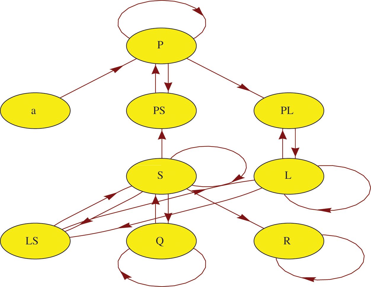
Figure 1: Schematic of the proposed model

Tab. 1 describes the parameters of the model.

The organization of the remainder of this paper is as follows. The stability of equilibrium points is studied in Section 2. Optimal control for the smoking model is discussed in Section 3. In Section 4, the second kind of Chebyshev polynomials and their properties are given. In Section 5, the numerical implementation is given. Finally, a conclusion is presented in Section 6.

2  Stability of Equilibrium Points

For the stability behavior of this model at E0=(1, 0, 0, 0, 0), we use transformations [36]:

U = 1-P, P = 1-U, L=L, S=S, Q=Q, R=R,

U*= −P*, L*=L*, S*=S*, Q*=Q*, R*=R*.

It follows that

dUdt=−aU+bS−bSU,dLdt=−aL+bL−bLU−cLS,dSdt=−aS−dS+cLS+fQ,dQdt=−aQ−fQ+ds−deS,dRdt=−aR+edS. (2.1)

The system (2.1) has

P1=(0, 0, 0, 0, 0), P2=(U*, L*, S*, Q*, R*), P3=(U**, L**, S**, Q**, R**),

P4=(U***, L***, S***, Q***, R***) and P5=(U****, L****, S****, Q****, R****),

where, U*=1-P*, U**=1-P**, U***=1-P*** and U****=1-P****.

Through Taylor approximation, the linearized form of the model is

[ X′Y′Z′V′W′ ]=B[ XYZVW ], (2.2)

where X=U-0, Y=L-0, Z=S-0, V=Q-0, W=R-0, and

B=[ -a          0             b            0              00        -a+b           0             0              00        -a-d            f               0               0 0          0           d-de         -a-f              00          0            ed            0             -a]. (2.3)

The stability of (2.1) is the same as the linearized stability (2.3). The stability of (2.3) depends on eigenvalues B. The point P1 is asymptotically locally stable if eigenvalues are real negative parts; conversely, P1 is unstable if at least one eigenvalue of B is a nonnegative real part. For details on stability see [56,63].

3  Optimal Control for Smoking Model

Consider the state presented (1.2), in R5, with control functions admissible [28–32]:

where Tf is the final time, and uV(.)  and  uR(.) are functions controls.

The objective function is defined as

J(uV(.),uR(.))=∫0Tf[AL(t)+BuV2(t)+CuR2(t)]dt, (3.1)

where A, B, and C represent the number of occasional smokers, the rate of contact between smokers and quitters, and temporarily who regain support to smoking, and rate of smoking quitting.

We minimize the objective function as follows [28–32]:

J(uV,uR)=∫0Tfηdt, (3.2)

which is subjected to the constraint

DP=ξ1,DL=ξ2,DS=ξ3,DQ=ξ4,DR=ξ5,ξk=ξ,k=1,2,3,4,5. (3.3)

The following initial conditions are satisfied:

P=P0,L=L0,S=S0,Q=Q0,R=R0. (3.4)

OCP is defined, and we consider the following modified objective (cost) function:

J¯=∫0Tf[H−∑k=15λkξk]dt, (3.5)

where the Hamiltonian and control smoking objective functions are defined as

H=η+∑k=15λkξk, (3.6)

H=AL+BuE2+CuM2+λ1∗(a(1−P)−bPS)+λ2∗(−aL+bPL−cLS)+λ3∗(−(a+d)S+cLS+fQ)+λ4∗(−(a+f)Q+d(1−e)S)+λ5∗(−aR+edS). (3.7)

From (3.5) and (3.7), the conditions, necessary and sufficient for OPC are

Dλ1∗=∂H∂P,Dλ2∗=∂H∂L,Dλ3∗=∂H∂S,Dλ4∗=∂H∂Q,Dλ5∗=∂H∂R, (3.8)

0=∂H∂uk⇒0=∂H∂uE,0=∂H∂uM. (3.9)

DP=∂H∂λ1∗,DL=∂H∂λ2∗,DS=∂H∂λ3∗,DQ=∂H∂λ4∗,DR=∂H∂λ5∗. (3.10)

λk,(Tf) = 0. (3.11)

where λk, k = 1, 2, 3, 4, 5 are Lagrange multipliers. Eqs. (3.9)–(3.10) clarify the conditions of the Hamiltonian for the OPC.

We construct a theorem similar to that presented in [28–32], [44–47].

Theorem 1.

If uV and uR are optimal controls with states corresponding to P∗,L∗,S∗,Q∗andR∗, there work out adjoint variables λk∗,k = 1,2,3,4,5, accepts:

Co-state equation

Dλ1∗=λ1∗(−a−bS∗)+λ2∗(bL∗), (3.12)

Dλ2∗=A+λ2∗(−a+bP∗)+λ3∗(cS∗), (3.13)

Dλ3∗=λ1∗(−bP∗)+λ2∗(−cL∗)+λ3∗(−a−d+cL∗)+λ4∗(d−ed)+λ5∗(ed), (3.14)

Dλ4∗=λ3∗(f)+λ4∗(−a−f), (3.15)

Dλ5*=λ5*(−a). (3.16)

With condition transversality:

λk∗(Tf) = 0. (3.17)

Optimality conditions

H=min0≤uV∗,uR∗≤1⁡H, (3.18)

Therefore, the function controls uV∗,uR∗ are given by

uV∗= Q∗[λ4∗−λ3∗]2B, (3.19)

uR∗= S∗[λ3∗−λ4∗−eλ5∗]2C, (3.20)

uV∗= min{1,max{0,Q∗[λ4∗−λ3∗]2B}}, (3.21)

uR∗= min{1,max{0,S∗[λ3∗−λ4∗−eλ5∗]2C}}. (3.22)

For more on optimal controls for solving models, see [29–32,44,47].

4  Properties of the Second Kind of Chebyshev Polynomials

4.1 Second Kind of Chebyshev Polynomials

Chebyshev polynomials Zn(y) of the second kind are rectangular polynomials of stage n in x presented on the interval [−1, 1] [34,35,57–59]:

Zn(y) = sin(n + 1)θsinθ, where y = cosθ and θ ∈ [0, π].

Polynomials have rectangular with rating to the products indoor

〈 Zn(y),Zm(y) 〉=∫−111−y2Zn(y)Zm(y)dy={ 0, n≠m,π2, n=m, (4.1)

where 1−y2 is a weight function.

Zn(y) can be generated by recurring relations

Zn(y) = 2y Zn−1(y) − Zn−2(y), n = 2, 3, …, n, with Z0(y) = 1. Z1(y) = 2y.

The analytical form Zn(y) of stage n is given by [34]:

Zn(y)=∑i=0⌈n2⌉(−1)i(in−i)(2y)n−2i=∑i=0⌈π2⌉(−1)i2n−2iΓ(n−i+1)yn−2iΓ(i+1)Γ(n−2i+1),n>0. (4.2)

Here, ⌈n2⌉ is part integral n/2.

4.2 Second Kind of Shifted Chebyshev Polynomials

On the interval y ∈ [0, 1], Zn∗(y) is defined via substituting a change variable z = 2y − 1. Hence, Zn∗(y) is defined as [33–35] Zn∗(y) = Zn(2y−1), and satisfies the following relation: 2yZn−1∗(y2) = Z2n−1(y).

The following inner product is orthogonal on the interval [0, 1]:

〈 Zn∗(y),Zm∗(y) 〉=∫01y−y2Zn∗(y)Zm∗(y)dy={ 0, n≠m,π8, n=m, (4.3)

with weight function y−y2.Zn∗(y) can be produced via recurring relations

Zn∗(y) = 2(2y−1)Zn−1∗(y)−Zn−2∗(y),n = 2,3,…,n, with Z0∗(y) = 1,Z0∗(y) = 4y−2.

The following formula represents the analytical

Zr∗(y)=∑j=0r(−1)j22r−2jΓ(2r−j+2)yr−jΓ(j+1)Γ(2r−2j+2),r>0, (4.4)

The solution of this model can be written as Z∗(y) .

Let g(y) be a square integral in [0, 1], and then the second kind of shifted Chebyshev polynomials can be represented as follows:

g(y)=∑i=0∞aiZi∗(y), (4.5)

The coefficients aj, j = 0, 1, …, are expressed as

ai=2π∫−11g(y+12)1−y2Zi(y)dy, (4.6)

or

ai=8π∫01g(y)y−y2Zi∗(y)dy, (4.6a)

We use only the (r + 1) terms. Then,

gr(y)=∑i=0raiZi∗(y). (4.7)

Using the practice to construct an integral collocation style then z(y) as follows [33]:

dkz(y)dxk≅∑n=0ranZn∗(y)=∑n=0ranwnk(y). (4.8)

By integrating (4.8), we can obtain the following:

dk−1z(y)dyn−1≅∑n=0ranwnk−1(y)+c1 (4.9)

dk−2z(y)dyn−2≅∑n=0ranwn(k−2)(y)+c1y+c2,… (4.10)

dz(y)dx≅∑n=0ranwn(1)(y)+c1yk−2(k−2)!+c2yk−3(k−3)!+…+ck−2y+ck−1, (4.11)

z(y)=∑n=0ranwn(0)(y)+c1yk−1(k−1)!+c2yk−2(k−2)!+…+ck−1y+ck, (4.12)

From (4.8) and (4.12), we then have

wn(k)(y)=∑i=0n(−1)i22n−2iΓ(2n−i+2)yn−iΓ(i+1)Γ(2n−2i+2),wn(k−1)(y) = ∫wn(k)(y)dy = ∑i=0n(−1)i22n−2iΓ(2n−i + 2)yn−i+1Γ(i + 1)Γ(2n−2i + 2)(n−i + 1),wn(k−2)(y) = ∫wn(k−1)(y)dx = ∑i=0n(−1)i22n−2iΓ(2n−i + 2)yn−i+2Γ(i + 1)Γ(2n−2i + 2)(n−i + 1)(n−i + 2),wn(0)(y) = ∫wn(1)(y)dx = ∑i=0n(−1)i22n−2iΓ(2n−i + 2)yi+kΓ(i + 1)Γ(2n−2i + 2)…(i + k−1)(i + k). (4.13)

We presently register Eqs. (4.9)–(4.13) at  (r + 1) points  yp,  p = 0, 1, …, r  as follows:

dkz(yp)dyk= Ω(k)E^,dk−1z(yp)dyk−1= Ω(k−1)E^,…,dz(yp)dy= Ω(1)E^,z(yp) = Ω(0)E^, (4.14)

where E^ = [a0,a1,...,am,c1,c2,...cn]T , and  Ω(r), Ω(r−1), …, Ω(0)  are combined matrices.

5  Style Integral Collocation for Resolving the Nonlinear Smoking Model

In this section, we present the model's implementation through the following steps:

We first approximate the function using Eqs. (4.8)–(4.14) with  m = 5 , as follows:

dPdt≅∑n=05Anwn(1)(t),dLdt≅∑n=05Bnwn(1)(t),dSdt≅∑n=05Cnwn(1)(t),dQdt≅∑n=05Dnwn(1)(t),dRdt≅∑n=05Enwn(1)(t),P(t)≅∑n=05Anwn(0)(t)+c1,L(t)≅∑n=05Bnwn(0)(t)+c2,S(t)≅∑n=05Cnwn(0)(t)+c3,Q(t)≅∑n=05Qnwn(0)(t)+c4,R(t)≅∑n=05Enwn(0)(t)+c5, (5.1)

where wn(0)(t) and wn(1)(t) are expressed as

Then, the nonlinear smoking model (1.1) is transformed to

∑n=05Anwn(1)(t)=a(1−∑n=05Anwn(0)(t)+c1)−b(∑n=05Anwn(0)(t)+c1)(∑n=05Bnwn(0)(t)+c2),∑n=05Bnwn(1)(t)=−a(∑n=05Bnwn(0)(t)+c2)+b(∑n=05Anwn(0)(t)+c1)(∑n=05Bnwn(0)(t)+c2)−c(∑n=05Bnwn(0)(t)+c2)(∑n=05Cnwn(0)(t)+c3),∑n=05Cnwn(1)(t)=−(a+d)(∑n=05Cnwn(0)(t)+c3)+c(∑n=05Bnwn(0)(t)+c2)(∑n=05Cnwn(0)(t)+c3)+f(∑n=05Dnwn(0)(t)+c4),∑n=05Dnwn(1)(t)=−(a+f)(∑n=05Dnwn(0)(t)+c4)+(d−de)(∑n=05Cnwn(0)(t)+c3),∑n=05Enwn(1)(t)=−a(∑n=05Enwn(0)(t)+c5)+ed(∑n=05Cnwn(0)(t)+c3). (5.2)

Now, we collocate Eq. (5.2) at (r + 1 = 6)  points ty, y = 0 − 5;  as follows:

∑n=05Anwn(1)(ty)=a(1−∑n=05Anwn(0)(ty)+c1)−b(∑n=05Anwn(0)(ty)+c1)(∑n=05Bnwn(0)(ty)+c2),∑n=05Bnwn(1)(ty)=−a(∑n=05Bnwn(0)(ty)+c2)+b(∑n=05Anwn(0)(ty)+c1)(∑n=05Bnwn(0)(ty)+c2)−c(∑n=05Bnwn(0)(ty)+c2)(∑n=05Cnwn(0)(ty)+c3),∑n=05Cnwn(1)(tp)=−(a+d)(∑n=05Cnwn(0)(tp)+c3)+c(∑n=05Bnwn(0)(tp)+c2)(∑n=05Cnwn(0)(tp)+c3)+f(∑n=05Dnwn(0)(tp)+c4),∑n=05Dnwn(1)(tp)=−(a+f)(∑n=05Dnwn(0)(tp)+c4)+(d−de)(∑n=05Cnwn(0)(tp)+c3),∑n=05Enwn(1)(tp)=−a(∑n=05Enwn(0)(tp)+c5)+ed(∑n=05Cnwn(0)(tp)+c3). (5.3)

The roots of shifted Chebyshev polynomial Z6∗(t).

(ii) By putting the initial Eqs. (1.2) into (5.1), we can obtain five equations.

Eqs. (5.1) and (5.3) obtained in step (ii) represent nonlinear algebraic system equations.

(iii) We use Newton's iteration to resolve the system and solve for the unknowns.

Figs. 2–4 show the nonlinear smoking model's behavior before control.

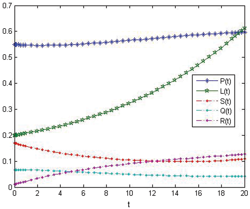
Figure 2: The approximate solution of variables about (ICSM) at r = 5 before control

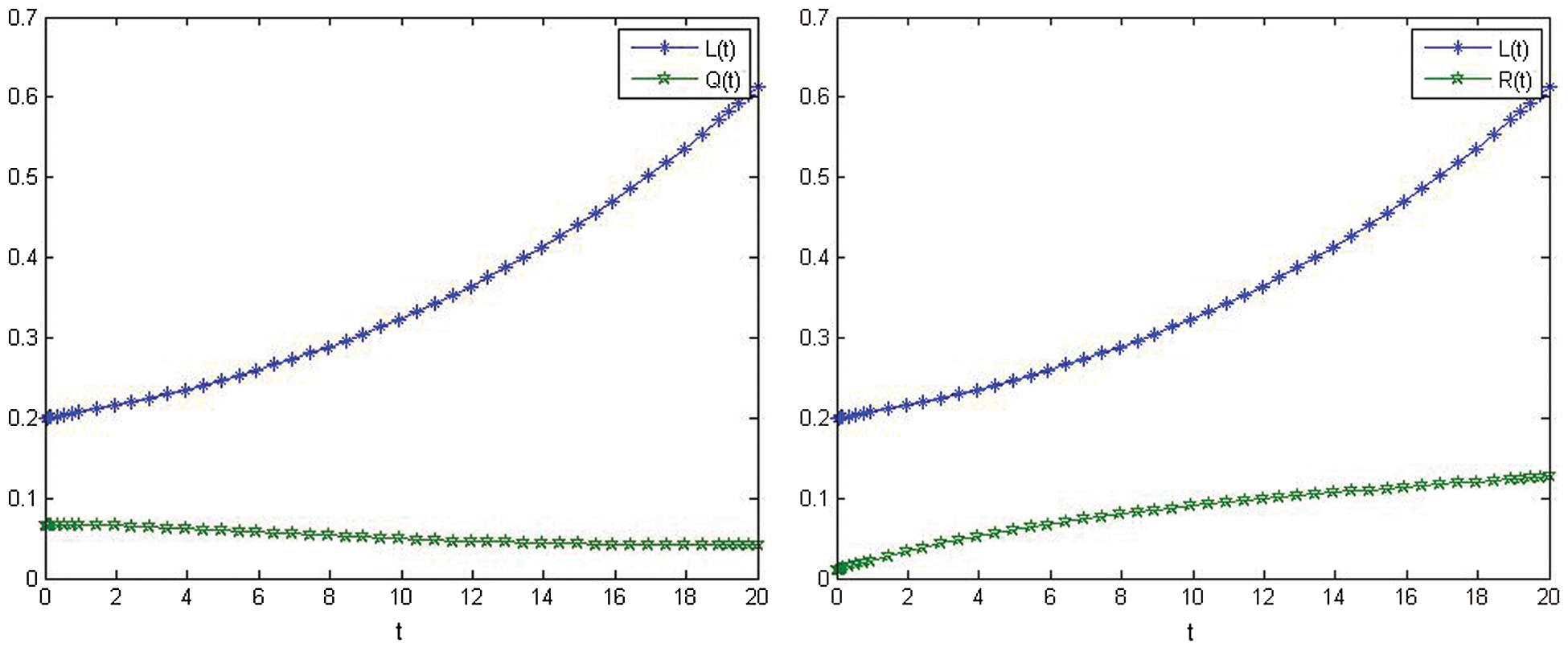
Figure 3: The relationship between L(t) and Q(t) before control. The relationship between L(t) and R(t) before control

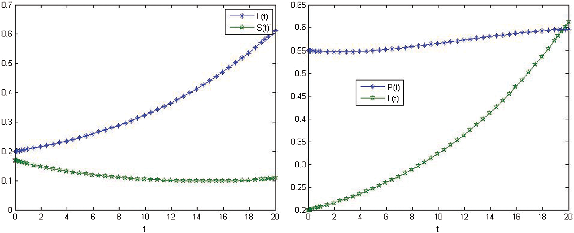
Figure 4: Relationship between L(t) and S(t) before control. Relationship between P(t) and L(t) before control

Figs. 5–8, show the show the nonlinear smoking model's behavior after control.

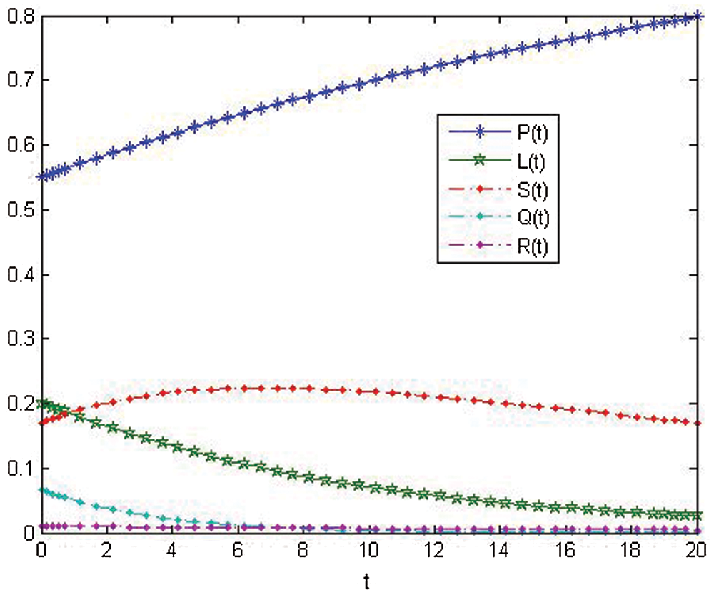
Figure 5: Approximate solution of variables about (ICSM) at r = 5 after control

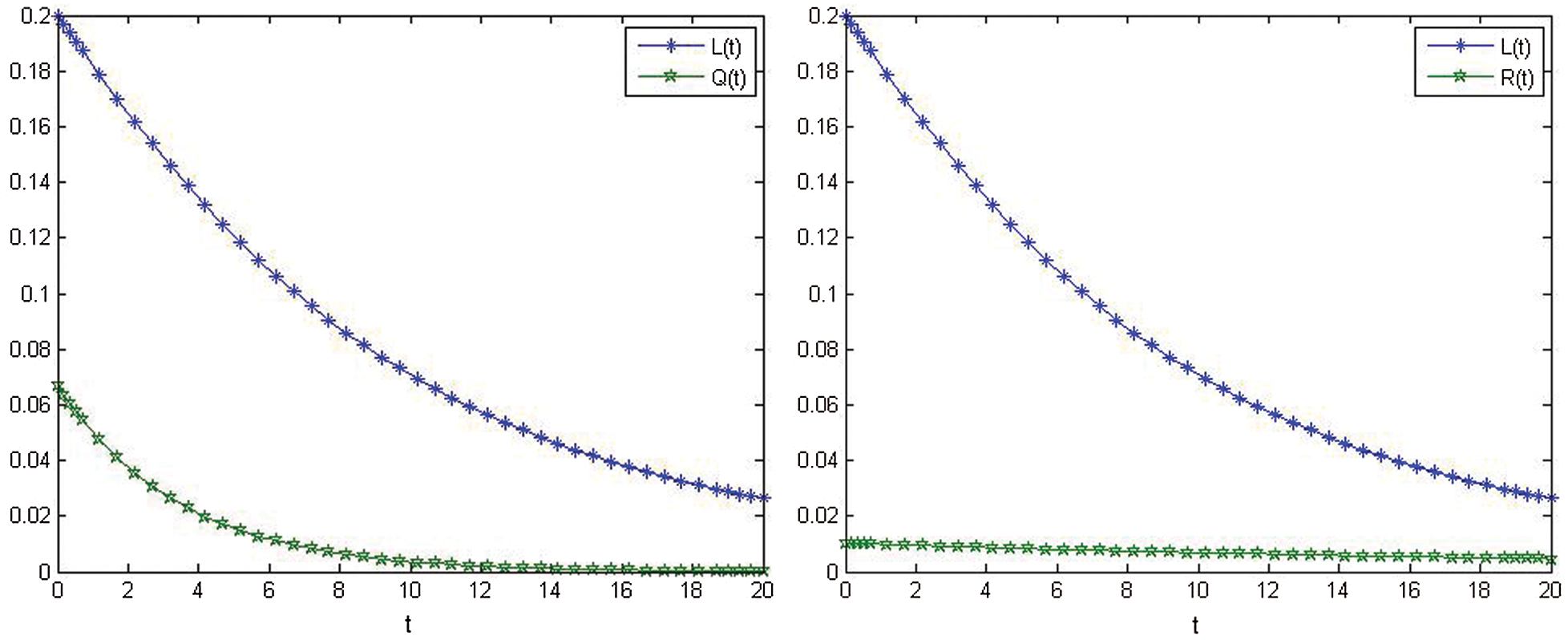
Figure 6: Relationship between L(t) and Q(t) after control. Relationship between L(t) and R(t) after control

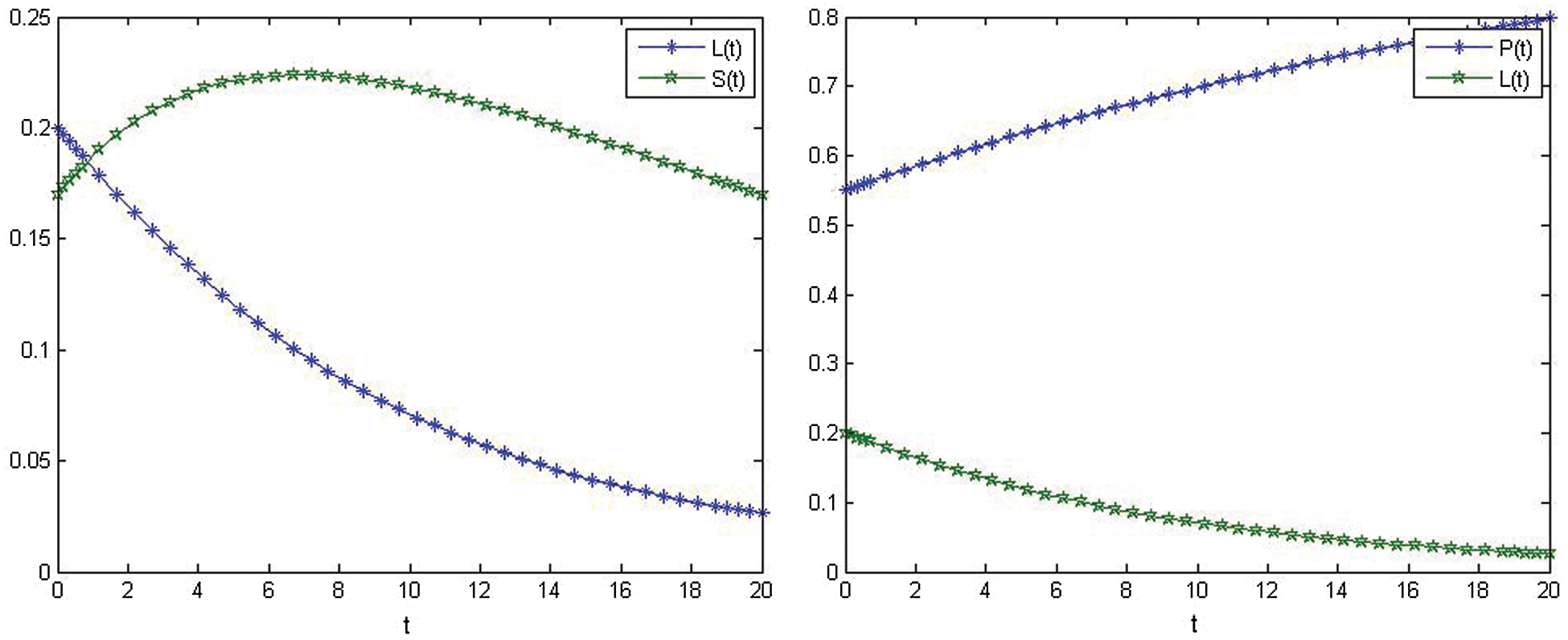
Figure 7: Relationship on L(t) and S(t) after control. Relationship on P(t) and L(t) after control

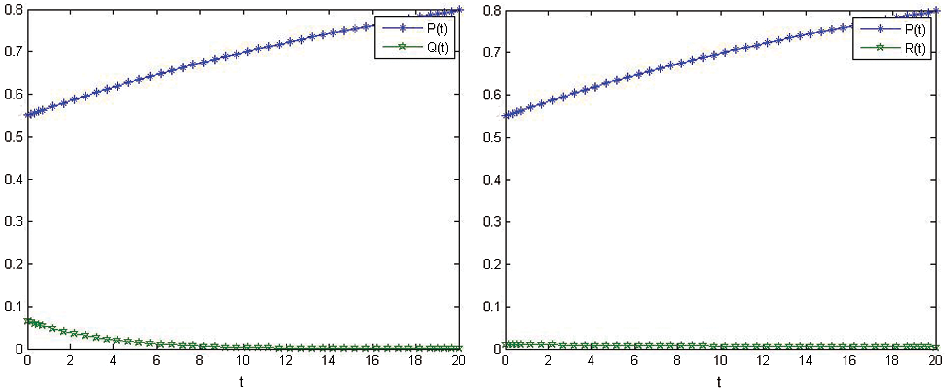
Figure 8: Relationship between P(t) and Q(t) after control. Relationship between P(t) and R(t) after control

6  Conclusions

In this manuscript, a mathematical nonlinear smoking model is studied. The optimal control of this smoking model is discussed. The stability of the equilibrium point is calculated, and a schematic of the proposed model is presented. Moreover, the integral collocation style is used to obtain the approximate solutions of the model. ICM using the shifted Chebyshev polynomials of the second kind is a new technique for solving these problems. Under the application with the necessary optimality conditions, we have studied the problem control with numerical techniques for the simulation. Moreover, a numerical method and its stability is discussed.

Acknowledgement: The authors are grateful for Taif University. Taif University researchers support project number (TURSP-2020/160), Taif University, Taif, Saudi Arabia.

Funding Statement: This manuscript has been funded through “Taif University's Researchers Supporting Project Number (TURSP-2020/160), Taif University, Taif, Saudi Arabia”.

Conflicts of Interest: The authors declare that there are no conflicts of interest.

References

 1.  A. H. Mokdad, J. S. Marks, D. F. Stroup and J. L. Gerberding, “Actual causes of death in the United States,” JAMA, vol. 291, pp. 1238–1245, 2004. [Google Scholar]

 2.  O. K. Ham, “Stages and processes of smoking cessation among adolescents,” Western Journal of Nursing Research, vol. 29, pp. 301–315, 2007. [Google Scholar]

 3.  V. S. Erturk. G. Zaman and S. Momani, “A numericl analytic method for approximating a giving up smoking model containing fractional derivatives,” Computer and Mathematics with Applications, vol. 64, no. 2, pp. 3068–3074, 2012. [Google Scholar]

 4.  J. Singh, D. Kumar, M. Al-Qurashi and D. Baleanu, “A new fractional model for giving up smoking dynamics,” Advances in Difference Equations, vol. 2017, pp. 1–16, 2017. [Google Scholar]

 5.  F. Haq, K. Shah. G. Rahman and M. Shahzad, “Numerical solution of fractional order smoking model via laplace adomian decomposition method,” Alexandria Engineering Journal, vol. 57, no. 2, pp. 1061–1069, 2018. [Google Scholar]

 6.  A. M. A. El-Sayed and S. M. Salman, “On a discretization process of fractional order riccati's differential equation,” Journal of Fractional Calculus and Applied Analysis, vol. 4, pp. 251–259, 2013. [Google Scholar]

 7.  A. A. Elsadany and A. E. Matouk, “Dynamical behaviors of fractional-order lotka-voltera predator-prey model and its discretization,” Applied Mathematics and Computation, vol. 49, pp. 49, pp. 269–283, 2015. [Google Scholar]

 8.  M. Khalid, F. S. Khan and A. Iqbal, “Perturbation iteration algorithm to solve fractional giving up smoking mathematical model,” International Journal of Computer Applications, vol. 142, no. 9, pp. 1–6, 2016. [Google Scholar]

 9.  G. Zaman, “Optimal campaign in the smoking dynamics,” Computational and Math. Methods in Medicine, vol. 2011, pp. 1–9, 2011. [Google Scholar]

10. G. Zaman, “Qualitative behavior of giving up smoking models,” Bulletin of the Malaysian Mathematical Sciences Socitey, vol. 34, no. 2, pp. 403–415, 2011. [Google Scholar]

11. J. L. Lubin and N. E. Cporaso, “Cigarette smoking and lung cancer: Modeling total exposure and intensity cancer epidemiology, “Biomarkers and Prevention, vol. 15, no. 3, pp. 517–523, 2006. [Google Scholar]

12. Y. A. Amer, A. M. S. Mahdy and E. S. M. Youssef, “Solving systems of fractional differential equations using sumudu transform method,” Asian Research Journal of Mathematics, vol. 7, no. 2, pp. 1–15, 2017. [Google Scholar]

13. A. Zeb., I. Chohan and G. Zaman, “The homotopy analysis method for approximating of giving up smoking model in fractional order,” Applied Mathematics, vol. 3, pp. 914–919, 2012. [Google Scholar]

14. Z. Alkhudhari, S. Al-Sheikh and S. Al-Tuwairqi, “Global dynamics of mathematical model on smoking,” Applied Mathematics, vol. 2014, pp. 914–919, 2014. [Google Scholar]

15. A. A. M. Arafa, S. Z. Rida and H. M. Ali, “Generalized mittag-leffler function method for solving lorenz system,” International Journal of Innovation and Applied Studies, vol. 3, pp. 105–111, 2013. [Google Scholar]

16. A. M. S. Mahdy, M. S. Mohamed, K. Lotfy, M. Kadry and A. El-Bary, “Plasma-elastic-thermal propagation of a rotator semiconductor magneto-electric medium during microtemperature and photothermal excitation processes subjected to mechanical ramp type,” Waves in Random and Complex Media, pp. 1–21, 2020. [Google Scholar]

17. S. Z. Rida and A. A. M. Arafa, “New method for solving linear fractional differential equations,” International Journal of Differential Equations, vol. 2011, pp. 1–8, 2011. [Google Scholar]

18. I. Podlubny, “Fractional Differential Equations,” San Diego, CA: Academic Press, 1999. [Google Scholar]

19. A. M. S. Mahdy, K. A. Gepreel, Kh. Lotfy and A. A. El-Bary, “A numerical method for solving the rubella ailment disease model,” International Journal of Modern Physics C, vol. 32, no. 7, pp. 1–15, 2021. [Google Scholar]

20. F. Haq, K. Shah, G. Rahman and M. Shahzad, “Numerical solution of fractional order smoking model via laplace adomian decomposition method,” Alexandria Engineering Journal, vol. 57, no. 2, pp. 1061–1069, 2018. [Google Scholar]

21. S. Momani and Z. Odibat, “Numerical approach to differential equations of fractional order,” Journal of Computational and Applied Mathematics, vol. 207, pp. 96–110, 2007. [Google Scholar]

22. S. Deniz and N. Bildik, “Comparison of adomian decomposition method and taylor matrix method in solving different kinds of partial differential equations,” International Journal of Modeling and Optimization, vol. 4, no. 4, pp. 292–298, 2014. [Google Scholar]

23. H. Bulut, H. M. Baskonus and F. B. M. Belgacem, “The analytical solutions of some fractional ordinary differential equations by sumudu transform method,” Abstract Applied Analysis, vol. 2013, pp. 1–6, 2013. [Google Scholar]

24. S. Rathore, D. Kumar, J. Singh and S. Gupta, “Homotopy analysis sumudu transform method for nonlinear equations,” International Journal of Industrial Mathematics, vol. 4, no. 4, pp. 1–13, 2012. [Google Scholar]

25. J. Singh and D. Kumar, “Homotopy perturbation sumudu transform method for nonlinear equations,” Advances in Theoretical and Applied Mechanics, vol. 4, no. 4, pp. 165–175, 2011. [Google Scholar]

26. A. M. S. Mahdy, Y. A. Amer, M. S. Mohamed and E. Sobhy, “General fractional financial models of awareness with caputo–Fabrizio derivative,” Advances in Mechanical Engineering, vol. 12, no. 11, pp. 1–9, 2020. [Google Scholar]

27. H. Schmid and A. Huber, “Analysis of switched-capacitor circuits using driving-point signal-flowgraphs,” AnalogIntegr Circ Sig Process, vol. 96, pp. 495–507, 2018. [Google Scholar]

28. A. M. S. Mahdy and M. Higazy, “Numerical different methods for solving the nonlinear biochemical reaction model,” International Journal of Applied and Computational Mathematics, vol. 5, no. 6, pp. 1–17, 2019. [Google Scholar]

29. N. H. Sweilam and S. M. Al-Mekhlafi, “Optimal control for a nonlinear mathematical model of tumor under immune suppression a numerical approach,” Optimal Control Applications and Methods, vol. 39, pp. 1581–1596, 2018. [Google Scholar]

30. N. H. Sweilam, S. M. Al-Mekhlafi and D. Baleanu, “Optimal control for a fractional tuberculosis infection model including the impact of diabetes and resistant strains,” Journal of Advanced Research, vol. 17, pp. 125–137, 2019. [Google Scholar]

31. N. H. Sweilam, O. M. Saad and D. G. Mohamed, “Fractional optimal control in transmission dynamics of west Nile model with state and control time delay a numerical approach,” Advances in Difference Equations, vol. 2019, no. 210, pp. 1–25, 2019. [Google Scholar]

32. N. H. Sweilam, O. M. Saad and D. G. Mohamed, “Numerical treatments of the tranmission dynamics of west Nile virus and it's optimal control,” Electronic Journal of Mathematical Analysis and Applications, vol. 7, no. 2, pp. 9–38, 2019. [Google Scholar]

33. A. M. S. Mahdy and N. A. H. Mukhtar, “Second kind shifted chebyshev polynomials for solving the model nonlinear ODEs,” American Journal of Computational Mathematics, vol. 7, no. 4, pp. 391–401, 2017. [Google Scholar]

34. N. H. Sweilam, A. M. Nagy and A. A. Sayed, “Second kind shifted chebyshev polynomials for solving space fractional order diffusion equation,” chaos,” Solitons and Fractals, vol. 73, pp. 141–147, 2015. [Google Scholar]

35. J. C. Mason and D. C. Handscomb, “Chebyshev Polynomials,” Chapman and Hall, New York, NY, CRC, Boca Raton, 2003. [Google Scholar]

36. I. A. Moneim and G. A. Mosa, “Modelling the hepatitis C with different types of virus genome,” Computational and Mathematical Methods in Medicine, vol. 7, no. 1, pp. 3–13, 2006. [Google Scholar]

37. J. G. Liu, X. J. Yang, Y. Y. Feng and P. Cui, “On the (N+1)-dimensional local fractional reduced differential transform method and its applications‏,” Mathematical Methods in the Applied Sciences, vol. 43, no. 15, pp. 8856–8866, 2020. [Google Scholar]

38. J. G. Liu, X. J. Yang and Y. Y. Feng, “Analytical solutions of some integral fractional differential–difference equations,” Modern Physics Letters B, vol. 34, no. 1, pp. 205009, 2020. [Google Scholar]

39. J. G. Liu, X. J. Yang, Y. Y. Feng and M. Iqbal‏, “Group analysis to the time fractional nonlinear wave equation,” International Journal of Mathematics, vol. 31, no. 4, pp. 2050029, 2020. [Google Scholar]

A. M. S. Mahdy, “Numerical studies for solving fractional integro-differential equations,” Journal of Ocean Engineering and Science, vol. 3, no. 2, pp. 127–132, 2018. [Google Scholar]

41. H. Khan, R. Shah, P. Kumam, D. Baleanu and M. Arif‏, “Laplace decomposition for solving nonlinear system of fractional order partial differential equations‏,” Advances in Difference Equations, vol. 2020, no. 1, pp. 1–18, 2020. [Google Scholar]

42. A. Ghaffar, A. Ali, S. Ahmed, S. Akram, D. Baleanu et al., “A novel analytical technique to obtain the solitary solutions for nonlinear evolution equation of fractional order,” ‏Advances in Difference Equations, vol. 2020, no. 1, pp. 1–15, 2020. [Google Scholar]

43. D. Baleanu, H. Mohammadi and S. Rezapour, “A fractional differential equation model for the COVID-19 transmission by using the caputo–Fabrizio derivative‏,” Advances in Difference Equations, vol. 2020, no. 1, pp. 1–27, 2020. [Google Scholar]

44. N. H. Sweilam, S. M. Al-Mekhlafi, T. Assiri and A. Atangana, “Optimal control for cancer treatment mathematical model using atangana–Baleanu–Caputo fractional derivative‏,” Advances in Difference Equations, vol. 2020, no. 1, pp. 1–21, 2020. [Google Scholar]

45. N. H. Sweilam, D. M. El-Sakout and M. M. Muttardi, “Compact finite difference method to numerically solving a stochastic fractional advection-diffusion equation‏,” Advances in Difference Equations, vol. 2020, no. 1, pp. 1–20, 2020. [Google Scholar]

46. K. A. Gepreel, M. Higazy and A. M. S. Mahdy, “Optimal control, signal flow graph, and system electronic circuit realization for nonlinear anopheles mosquito model,” International Journal of Modern Physics C, vol. 31, no. 9, pp. 1–18, 2020. [Google Scholar]

47. A. M. S. Mahdy, H. Higazy, K. A. Gepreel and A. A. A. El-dahdouh, “Optimal control and bifurcation diagram for a model nonlinear fractional SIRC,” Alexandria Engineering Journal, vol. 59, no. 5, pp. 3481–3501, 2020. [Google Scholar]

48. Y. A. Amer, A. M. S. Mahdy and H. A. R. Namoos, “Reduced differential transform method for solving fractional-order biological systems,” Journal of Engineering and Applied Sciences, vol. 13, no. 20, pp. 8489–8493, 2018. [Google Scholar]

49. Y. A. Amer, A. M. S. Mahdy, R. T. Shwayaa and E. S. M. Youssef, “Laplace transform method for solving nonlinear biochemical reaction model and nonlinear emden-fowler system,” Journal of Engineering and Applied Sciences, vol. 13, no. 17, pp. 7388–7394, 2018. [Google Scholar]

50. M. M. Khader, N. H. Sweilam and A. M. S. Mahdy, “The chebyshev collection method for solving fractional order klein-gordon equation,” WSEAS Transactions on Mathematics, vol. 13, pp. 31–38, 2014. [Google Scholar]

51. A. M. S. Mahdy, K. Lotfy, M. H. Ahmed, A. El-Bary and E. A. Ismail, “Electromagnetic hall current effect and fractional heat order for micro temperature photo-excited semiconductor medium with laser pulses,” Results in Physics, vol. 17, pp. 1–9, 2020. [Google Scholar]

52. A. K. Khamis, K. Lotfy, A. A. El-Bary, A. M. S. Mahdy and M. H. Ahmed, “Thermal-piezoelectric problem of a semiconductor medium during photo-thermal excitation,” Waves in Random and Complex Media, pp. 1–15, 2020. [Google Scholar]

53. A. M. S. Mahdy, K. Lotfy, E. A. Ismail, A. A. El-Bary, M. Ahmed et al. “Analytical solutions of time-fractional heat order for a magneto-photothermal semiconductor medium with thomson effects and initial stress,” Results in Physics, vol. 18, pp. 1–11, 2020. [Google Scholar]

54. A. M. S. Mahdy, K. Lotfy, W. Hassan and A. A. El-Bary, “Analytical solution of magneto-photothermal theory during variable thermal conductivity of a semiconductor material due to pulse heat flux and volumetric heat source,” Waves in Random and Complex Media, pp. 1–19, 2020. [Google Scholar]

55. A. M. S. Mahdy and E. S. M. Youssef, “Numerical solution technique for solving isoperimetric variational problems,” International Journal of Modern Physics C, vol. 32, no. 1, pp. 1–14, 2021. [Google Scholar]

56. A. M. S. Mahdy, M. S. Mohamed, K. A. Gepreel, A. AL-Amiri and M. Higazy, “Dynamical characteristics and signal flow graph of nonlinear fractional smoking mathematical model,” Chaos, Solitons and Fractals, vol. 141, pp. 1–16, 2020. [Google Scholar]

57. E. H. Doha, A. H. Bhrawy and S. S. Ezz-Eldien, “Efficient chebyshev spectral methods for solving multi-term fractional orders differential equations,” Applied Mathematical Modelling, vol. 35, pp. 5662–5672, 2011. [Google Scholar]

58. E. H. Doha, A. H. Bhrawy and S. S. Ezz-Eldien, “A chebyshev spectral method based on operational matrix for initial and boundary value problems of fractional order,” Computers & Mathematics with Applications, vol. 62, pp. 2364–2373, 2011. [Google Scholar]

59. A. H. Bhrawy and M. A. Alshomrani, “Shifted legendre spectral method for fractional-order multi-point boundary value problems,” Advances in Difference Equations, vol. 2012, pp. 1–19, 2012. [Google Scholar]

60. A. M. S. Mahdy, “Numerical solutions for solving model time-fractional fokker–Planck equation,” Numerical Methods for Partial Differential Equations, vol. 37, no. 2, pp. 1120–1135, 2021. [Google Scholar]

61. A. Khan, H. Khan, J. F. Gómez-Aguilar and T. Abdeljawad, “Existence and hyers-ulam stability for a nonlinear singular fractional differential equations with mittag-leffler kernel,” Chaos, Solitons and Fractals, vol. 127, pp. 422–427, 2019. [Google Scholar]

62. A. Khan, J. F. Gómez-Aguilar, T. S. Khan and H. Khan, “Stability analysis and numerical solutions of fractional order HIV/AIDS model,” Chaos, Solitons and Fractals, vol. 122, pp. 119–128, 2019. [Google Scholar]

63. I. Ullah, S. Ahmad, Q. Al-Mdallal, Z. A. Khan, H. Khan et al., “Stability analysis of a dynamical model of tuberculosis with incomplete treatment,” Advances in Difference Equations, vol. 2020, no. 1, pp. 1–14, 2020. [Google Scholar]

64. K. A. Gepreel, A. M. S. Mahdy, M. S. Mohamed and A. Al-Amiri, “Reduced differential transform method for solving nonlinear biomathematics models,” Computers, Materials and Continua, vol. 61, no. 3, pp. 979–994, 2019. [Google Scholar]

65. Y. A. Amer, A. M. S. Mahdy and E. S. M. Youssef, “Solving fractional integro-differential equations by using sumudu transform method and hermite spectral collocation method,” Computers Materials and Continua, vol. 54, no. 2, pp. 161–180, 2018. [Google Scholar]

66. K. A. Gepreel, M. S. Mohamed, H. Alotaibi1 and A. M. S. Mahdy, “Dynamical behaviors of nonlinear coronavirus (COVID-19) model with numerical studies,” Computers Materials and Continua, vo. vol. 67, no. 1, pp. 675–686, 2021. [Google Scholar]

67. M. I. A. Othman and A. M. S. Mahdy, “Numerical studies for solving a free convection boundary–layer flow over a vertical plate,” Mechanics and Mechanical Engineering, vol. 22, no. 1, pp. 41–48, 2018. [Google Scholar]

68. H. H. Abdel-Halim, M. I. A. Othman and A. M. S. Mahdy, “Variational iteration method for solving twelve order boundary value problems,” Journal of Mathematical Analysis, vol. 3, no. 15, pp. 719–730, 2009. [Google Scholar]

69. A. M. S. Mahdy, N. H. Sweilam and M. Higazy, “Approximate solutions for solving nonlinear fractional order smoking model,” Alexandria Engineering Journal, vol. 59, no. 2, pp. 739–752, 2020. [Google Scholar]

70. I. H. A. Hassan, M. I. A. Othman and A. M. S. Mahdy, “Variational iteration method for solving: Twelve order boundary value problems,” International Journal of Mathematical Analysis, vol. 3, no. 13–16, pp. 719–730, 2009. [Google Scholar]

71. A. M. S. Mahdy, M. Higazy and M. S. Mohamed, “Optimal and memristor-based control of a nonlinear fractional tumor-immune model,” Computers, Materials & Continua, vol. 67, no. 3, pp. 3463–3486, 2021. [Google Scholar]

72. A. M. S. Mahdy, M. S. Mohamed, K. Lotfy, M. Alhazmi, A. A. El-Bary et al. “Numerical solution and dynamical behaviors for solving fractional nonlinear rubella ailment disease model,” Results in Physics, vol. 24, pp. 1–10, 2021. [Google Scholar]

This work is licensed under a Creative Commons Attribution 4.0 International License, which permits unrestricted use, distribution, and reproduction in any medium, provided the original work is properly cited.