Intelligent Automation & Soft Computing DOI:10.32604/iasc.2022.019997
Article

Mixed Moving Average-Cumulative Sum Control Chart for Monitoring Parameter Change

Nongnuch Saengsura, Saowanit Sukparungsee* and Yupaporn Areepong

Department of Applied Statistics, Faculty of Applied Science, King Mongkut’s University of Technology North Bangkok, Bangkok, 10800, Thailand
*Corresponding Author: Saowanit Sukparungsee. Email: saowanit.s@sci.kmutnb.ac.th
Received: 05 May 2021; Accepted: 18 June 2021

Abstract: In this research, we propose the new mixed control chart called the mixed Moving Average-Cumulative Sum (MA-CUSUM) control chart used for monitoring parameter changes in asymmetrical and symmetrical processes. Its efficiency was compared with that of the Shewhart, Cumulative Sum (CUSUM), Moving Average (MA), mixed Cumulative Sum-Moving Average (CUSUM-MA) and mixed Moving Average-Cumulative Sum (MA-CUSUM) control charts by using their average run lengths (ARLs), the standard deviation of the run length (SDRL), and median run length (MRL) via the Monte Carlo simulation (MC). The simulation results show that the MA-CUSUM control chart was more efficient than the other control charts for small-to-moderate parameter changes for all distributions tested. To compare their applicability to real-world situations, the control charts were applied to data for the River Nile flow from 1871–1930 and mine explosions in the UK from 1875–1951. It was found that the MA-CUSUM control chart could more quickly detect parameter changes than the other control charts.

Keywords: Average run length; mixed control chart; moving average-cumulative sum control chart; cumulative sum control chart; moving average control chart; cumulative sum control chart

1  Introduction

Controlling product quality is essential in the manufacturing industry, and themost popular and widely used tool is the statistical process control chart. The statistical process control chart is used to control, monitor, detect changes, and develop production processes by making them more consistent or increasing the production capacity limit while keeping the process under control to achieve the objectives of consumer’s needs and make the product meet the specific requirements. As well as in the manufacturing industry, control charts have been applied in various fields, such as environmental science, epidemiology and emerging diseases, telecommunication, economics, finance, etc.

Therefore, statistical process control charts are commonly used for detecting change in processes. As a result, many control charts were invented.

Shewhart [1] proposed the first use of a control chart (known as the Shewhart control chart) by applying statistical principles to control and detect large changes in the process mean. Later, Page [2] presented the cumulative sum (CUSUM) control chart using weighted historical data that is effective at detecting small-to-meoderate changes in process parameters. Roberts [3] proposed the exponentially weighted moving average (EWMA) control chart in which historical data are weighted, which is also effective at detecting small-to-moderate changes in process parameters. Khoo [4] developed moving average (MA) control chart by calculating the moving average by time period that could detect small changes and be applicable to data that from both continuous and discrete distributions. Abbas et al. [5] presented the combined EWMA-CUSUM control chart, which was more effective at detecting changes than the EWMA or CUSUM control charts separately. Khaliq et al. [6] presented the combined EWMA-Tukey’s (TCC) control chart and tested it using the mean run length as the benchmark performance measurement; their results indicate that EWMA-TCC was more effective at detecting changes than either the TCC or the EWMA control chart, although it did not perform well when the observations were skewed and the parameter change size was reduced. Riaz et al. [7] proposed the mixed Tukey’s EWMA-CUSUM (MEC-TCC) control chart to detect changes in the process mean and found that the new proposed control chart was more effective in detecting micro-changes than the combined EWMA-CUSUM parameter-based control chart, non-parametric combined control charts EWMA-TCC, CUSUM-TCC and TCC. Taboran et al. [8] proposed the new control chart: MA-EWMA to detect a change in process mean underlying asymmetric and symmetric processes, and compare the efficiency in monitoring the change with Shewhart, EWMA and MA control charts at the parameter change levels. Phanthuna et al. [9] proposed the explicit formula for evaluating the average runlength on a two-sided modified exponentially weighted moving average chart under the observations of a first-orderautoregressive process, referred to as AR(1) process, with an exponential white noise. Later, Sukparungsee et al. [10] proposed the mixed EWMA-MA control chart to detect changes in the mean of processes with underlying symmetric and asymmetric distributions; the results of performance comparison showed that the mixed EWMA-MA control chart performed better and detected process mean shifts more quickly than the individual Shewhart, MA, and EWMA control charts.

Herein, we proposed the new mixed control chart called the mixed Moving Average-Cumulative Sum control chart (MA-CUSUM) used for monitoring process parameter changes. We compared its efficiency with Shewhart, CUSUM, MA and CUSUM-MA control charts. We also compared the efficacies of the control charts by applying them to real data for the River Nile flow and mine explosions in the UK from 1875-1951.

2  The Control Charts Used in the Study

The control charts used in this study was the parametric control chart, which were CUSUM and MA control charts for small-to-moderate parameter changes. We presented new control chart, by mixing CUSUM and MA control charts (CUSUM-MA, MA-CUSUM) as follow.

2.1 The CUSUM Control Chart

The cumulative deviation from the target value is used in the derivation of this control chart. The CUSUM control chart is based on the following two statistics [11]:

Ci+=max(0,Ci−1++Xi−μ0−K1)Ci−=min(0,Ci−1−+Xi−μ0+K1)} (1)

where i is the time or sample number and Xi are independent and normally distributed observations for Xi∼N(μ0,σ0) , where μ0 and σ0 are the in-control mean and standard deviation, respectively. K1=k1σ0 is the reference value and is used for half of the shift, i.e., k1=δ2 , where δ is the number of shift given as δ=|μ1−μ0|σ0/σ0nn , where μ1 is the out-of-control mean, and n is the sample size. Statistics Ci+ and Ci− are the upper and lower CUSUM limits, respectively, and are plotted against to the control limit H1=h1σ0 . Initially, we set Ci+=C0−=0 .

2.2 The MA Control Chart

For each period ( w ), assume that individual measurements X1,X2,... , where Xi∼N(μ,σ2) , for i=1,2,... are obtained from the process. The MA statistic of span w at time i defined by Montgomery [12] is

MAi={Xi+Xi−1+Xi−2+...i,i<wXi+Xi−1+...+Xi−w+1w,i≥w (2)

The average of all measurements up to period i are defines for the MA. The respective mean and variance of the MA statistics, MAi are

E(MAi)=E(Xi)=μ0 (3)

and

Var(MAi)={σ02i,i<wσ02w,i≥w (4)

where μ0 denotes the in-control process mean. The control limits of the MA control chart are as follows:

UCL/LCL={μ0±K2σ0i,i<wμ0±K2σ0w,i≥w (5)

where K2 is a coefficient of control limits of MA control chart and μ0 and σ0 are the mean and standard deviation of the in-control process, respectively.

2.3 The Mixed CUSUM-MA (MCM) Control Chart

In this case, the CUSUM statistics in Eq. (1) are used as inputs for the MA control chart, resulting in

MCMi+={Ci++Ci−1++⋯i,i<wCi++Ci−1++⋯+Ci−w+1+w,i≥w (6)

and

MCMi−={Ci−+Ci−1−+⋯i,i<wCi−+Ci−1−+⋯+Ci−w+1−w,i≥w (7)

where w is the width of the MA control chart and Ci+ , Ci− are the CUSUM statistics.

The respective mean and variance of the CUSUM-MA (MCM) statistics are

E(MCMi+)=E(MCMi−)=μC=μX¯ (8)

and

Var(MCMi+)=Var(MCMi−)=σC2=σX¯2 (9)

The upper (UCL) and lower (LCL) control limits of the mixed CUSUM-MA (MCM) control chart are given by

UCL/LCL={μC±K3σCi,i<wμC±K3σCw,i≥w (10)

where K3 is a coefficient of the control limits of the mixed CUSUM-MA (MCM) control chart, μC and σC are the mean and standard deviation of the in-control process, respectively.

2.4 The Mixed MA-CUSUM (MMC) Control Chart

Contrary to the mixed CUSUM-MA control chart, the MA statistics in Eq. (2) are used as input for the CUSUM chart as follows:

MMCi+=max(0,MMCi−1++MAi−μ0−K4)MMCi−=min(0,MMCi−1−+MAi−μ0+K4)} (11)

where K4 is the time-varying reference value defined as

K4=k4×Var(MAi)={k4σ0i,i<wk4σ0w,i≥w (12)

MMCi+ and MMCi− are the upper and lower limits statistics, respectively, for the mixed MA-CUSUM (MMC) control chart. Next, these statistics are represented as a function of the control limit HMAi , which is defined as follows:

HMAi=hMA×Var(MAi)={hMAσ0i,i<whMAσ0w,i≥w (13)

where hMA is the coefficient used to set the default false alarm rate. Any value of MMC+ crossing control limit HMAi indicates an increase in the process mean, and if MMC− goes beyond HMAi for any value of i , then this will point toward a negative shift in the process.

3  Performance Measurement Evaluation

The average run length (ARL) [12] is widely used to compare the performances of control charts. It is average number of observations required to be monitored before an out-of-control process is detected for the first time. Performance is assessed by setting the value of ARL0 (the in-control process) and the obtaining ARL1 (the out-of-control process). The ARL is defined as

ARL=∑i=1NRLiN. (14)

Other criteria used for measuring the performance of the control charts in this study are the standard deviation of the run length (SDRL) [13] and the median of the run length (MRL) [14,15] which are respectively calculated as follows:

SDRL=∑i=1N(RLi−ARL)2N−1 (15)

and

MRL=Median(RL) (16)

where RLi is the number of samples before the process is out-of-control for the first time, i is the number of data simulations, and N is the number of experiment repetitions. In the current study, the following steps were excuted:

1) Set the sample size ( m ) for each round of the experiment at 5,000.

2) Set the number of the experiment repetition ( R ) to 200,000.

3) Set ARL0=370 for the in-control process.

4  Simulation Study Results

The performance of the presented MA-CUSUM control chart was compared with the Shewhart, CUSUM, MA, and CUSUM-MA control charts for in-control processes with observations following normal (0,1), Laplace (0,1), exponential (1) and gamma (4,1) distributions. Furthermore, a comparison of the performance in detecting a change of the control chart when the change was δ∈[−4,4] . The evaluation criteria to evaluate the efficiencies of the control charts were ARL1, SDRL and MRL, with the control chart with the lowest ARL1, SDRL and MRL being the most efficient.

Tab. 1 and Fig. 1 contain the simulation results for a process with observations following a normal distribution. When μ=0 , σ2=1 , the CUSUM control chart obtained K1=0.3866 for w=5,h=5,L=3 and ARL1, SDRL, and MRL values were lower than the others at parameter change levels -0.05, -0.10, -0.25, -0.50, -2.00, -3.00, -4.00, 0.05, 0.10, 0.25, 0.50, 2.00, 3.00, and 4.00. Meanwhile, the MA-CUSUM control chart obtained K4=0.6298 and ARL1, SDRL, and MRL values lower than the others at parameter change levels of -0.75, -1.00, -1.50, 0.75, 1.00, and 1.50.

Tab. 2 and Fig. 1 contain the simulation results for a process with observations following a Laplace distribution when α=0 , β=1 . The proposed MA-CUSUM control chart obtained K4=0.8418 and lower ARL1, SDRL, and MRL values than the others at all parameter change levels except for -4.00 and 4.00, when the MA control chart performed better.

Tab. 3 and Fig. 1 contain the simulation results for a process with observations following an exponential distribution. When λ=1 , the MA-CUSUM control chart obtained K4=0.7622 and lower ARL1, SDRL, and MRL values than the others at all change levels except for 2.00, 3.00, and 4.00, when the CUSUM control chart was better.

Tab. 4 and Fig. 1 contain the simulation results for a process with observations following a gamma distribution. When α=4 , β=1 , the MA-CUSUM control chart obtained K4=0.8663 and lower ARL1, SDRL, and MRL values than the others at all parameter change levels except for 3.00 and 4.00, when the CUSUM control was better.

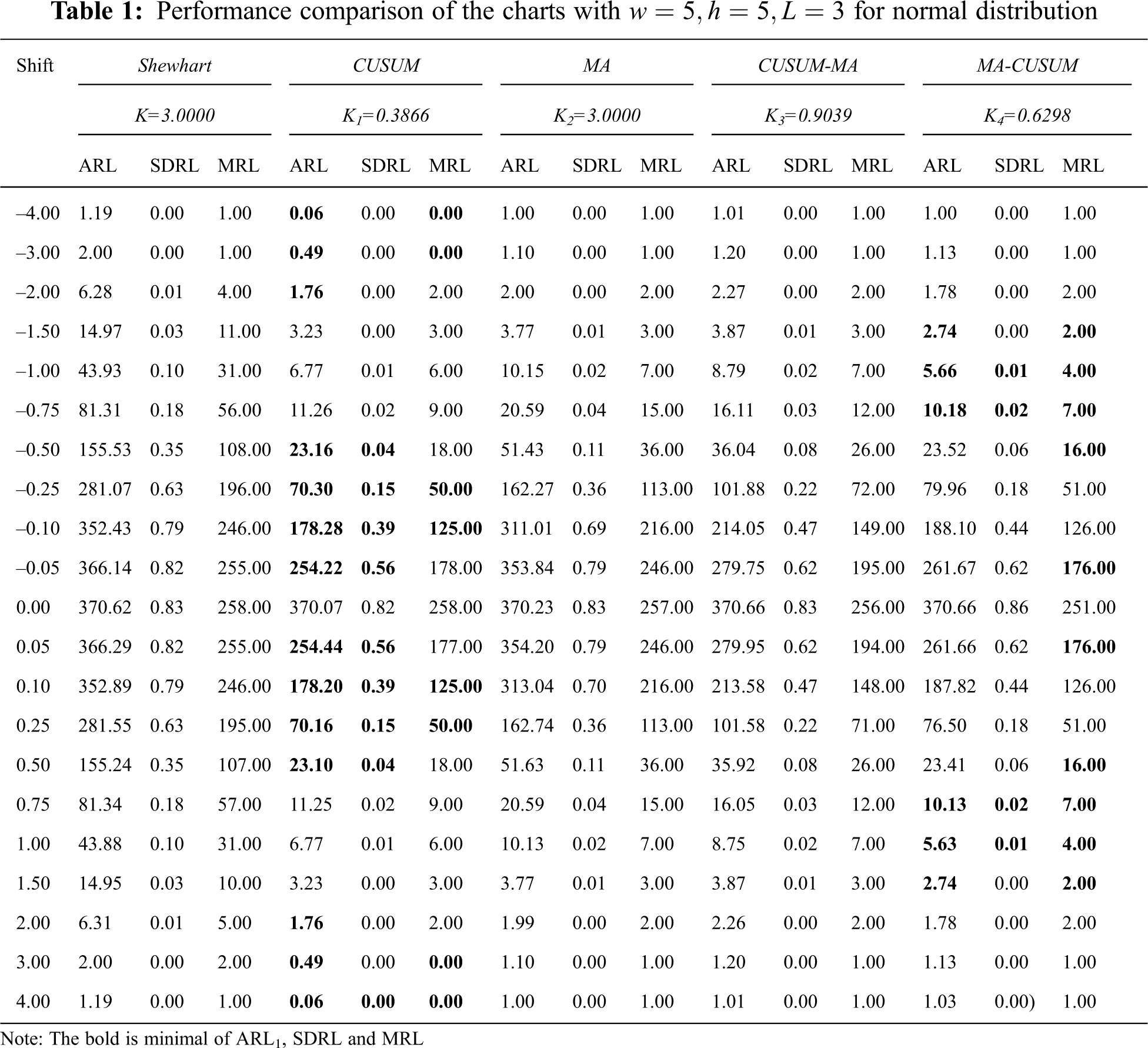
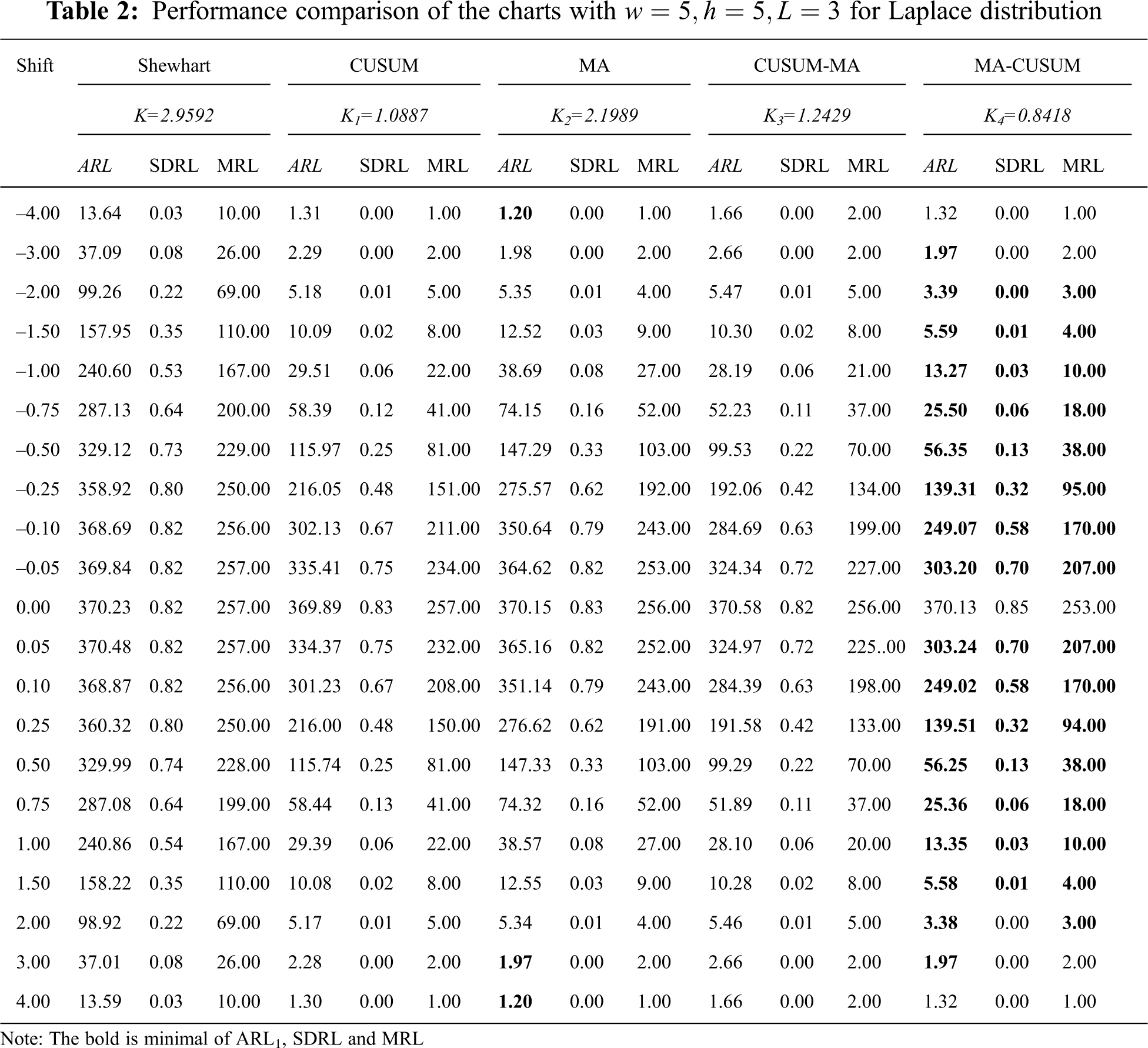
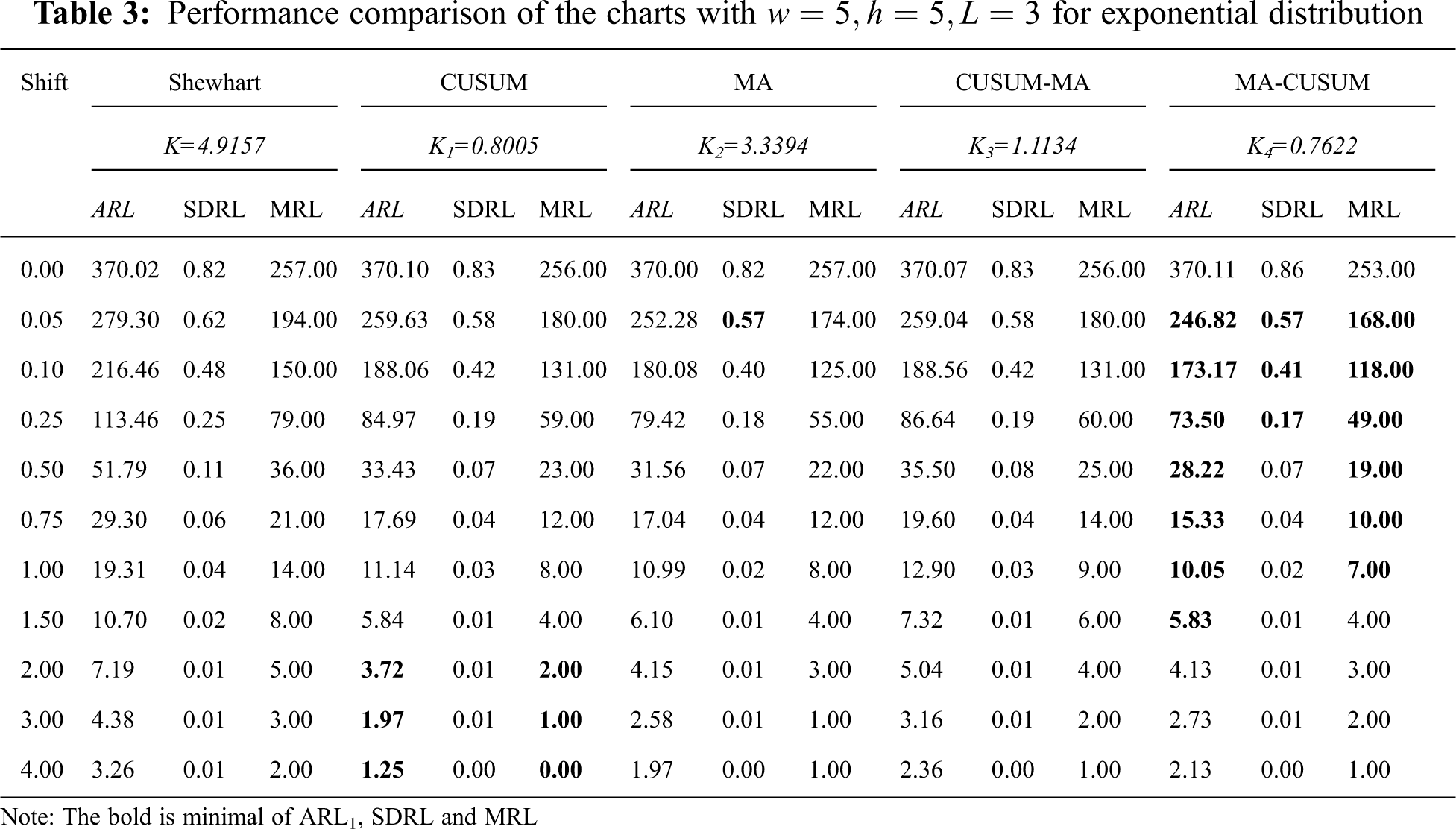
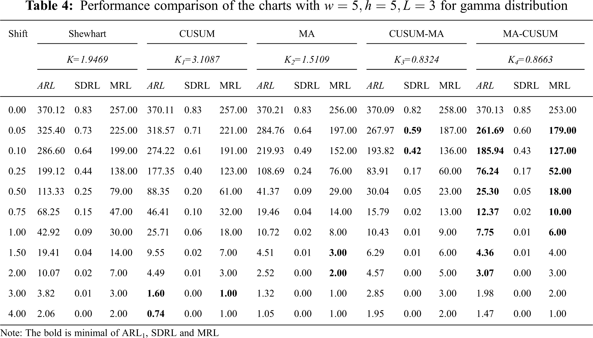
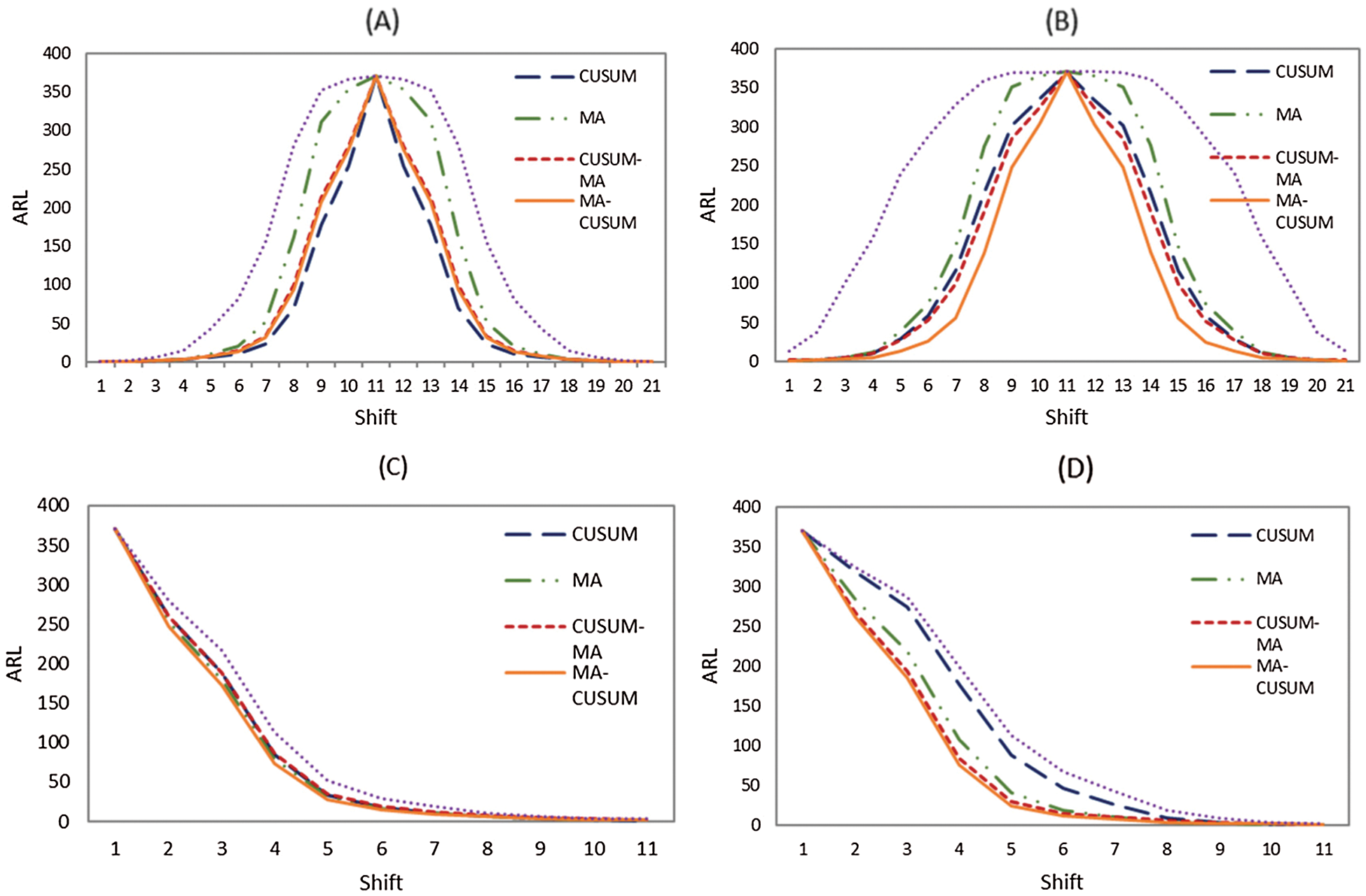
Figure 1: Average run length (ARL) curves of Shewhart, CUSUM, MA, CUSUM-MA, and MA-CUSUM for (A) normal distribution; (B) Laplace distribution; (C) exponential distribution and (D) gamma distribution

5  Performance Evaluation of the Control Charts with Real Data

For this evaluation, we considered two real datasets of River Nile flow data from 1871–1930 and mine explosions in the UK from 1875-1951 [16].

5.1 The River Nile Flow Data from 1871–1930

This data follows a normal distribution when the process is in control with a mean of 1,100 m3/s and a standard deviation of 125 m3/s. In 1900, the process had changed, with the mean decreasing to 850 m3/s. These data were applied to the Shewhart, CUSUM, MA, CUSUM-MA, and MA-CUSUM control charts, see Fig. 2. It can be concluded that the MA-CUSUM control chart was the quickest to detect a change in the River Nile flow in 1872, followed by the CUSUM control chart in 1896, the MA control chart in 1901 and the Shewhart control chart in 1902. The CUSUM-MA was unable to detect any change in the River Nile flow data.

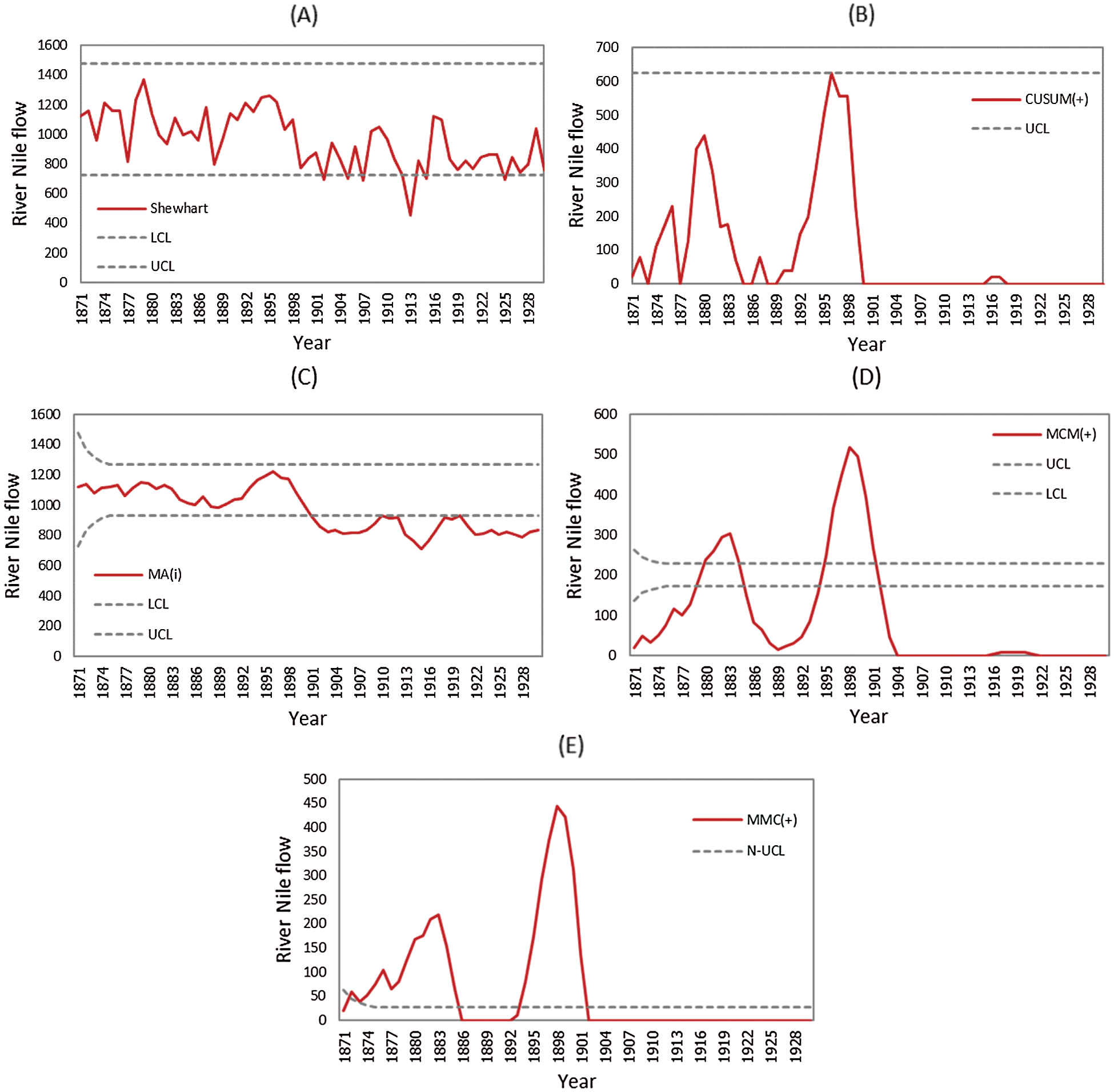
Figure 2: Comparison of detect the change of the Nile river flow between Shewhart, CUSUM, MA, CUSUM-MA and MA-CUSUM control charts, (A) Shewhart chart; (B) CUSUM chart; (C) MA chart; (D) CUSUM-MA chart and (E) MA-CUSUM chart

5.2 The Mine Explosion Data in the UK from 1875-1951

For the in-control process, the mean was 129 days/time. At the 51st obsevation, the process changed with a mean of 339 days/time. Again, we applied this data to all five control charts, see Fig. 3. This time, the MA-CUSUM control chart was the quickest to detect change in the mine explosion data at the 4th observation, followed by the CUSUM control chart at the 49th and the Shewhart and MA control charts at the 54th. Once again, the CUSUM-MA control chart not detect a change in the process mean.

6  Conclusions and Discussions

We proposed the mixed MA-CUSUM control chart, which is a combination of the MA and CUSUM control charts to detect shifts in the mean of processes that follow an asymmetrical distribution (exponential (1) and gamma (4,1)) and a symmetrical distribution (normal (0,1) and Laplace (0,1)) and ARL0 = 370. The results are summarized in Tab. 5.

For the process following a normal distribution, the MA-CUSUM control chart was the most efficient for process changes of −1.50≤δ≤−0.75 and 0.75≤δ≤1.50 , while the CUSUM chart was better than other for δ≤−2.0 , −0.50≤δ≤−0.05 , 0.05≤δ≤0.50 , and δ≥2.0 . For the process following a Laplace distribution, MA-CUSUM chart was the most efficient at all process change levels except for δ≤−2.0 and δ≥2.0 , when the MA control chart was better than the others. For the process following an exponential distribution, the MA-CUSUM control chart was more than efficient than others for 0.05≤δ≤0.50 and 0.75≤δ≤1.50 , while the CUSUM control chart was the better for δ≥2.0 . For the process following a gamma distribution, the MA-CUSUM control chart was more efficient than the others for 0.05≤δ≤0.50 and 0.75≤δ≤1.50 , while the CUSUM control chart was the best for δ≥2.0 .

For the River Nile flow dataset, the MA-CUSUM control chart was the quickest at detecting a change in the process mean in 1872, while for the mine explosion dataset, the MA-CUSUM control chart was the quickest. Indeed, the proposed MA-CUSUM control chart was more efficient than the MME-TCC in Taboran et al. [17] with the same dataset.

In further research studies, we plan to extend the efficiency comparision of the control chart, with alternative methods for determining the ARL and application examples with real data following different distributions.

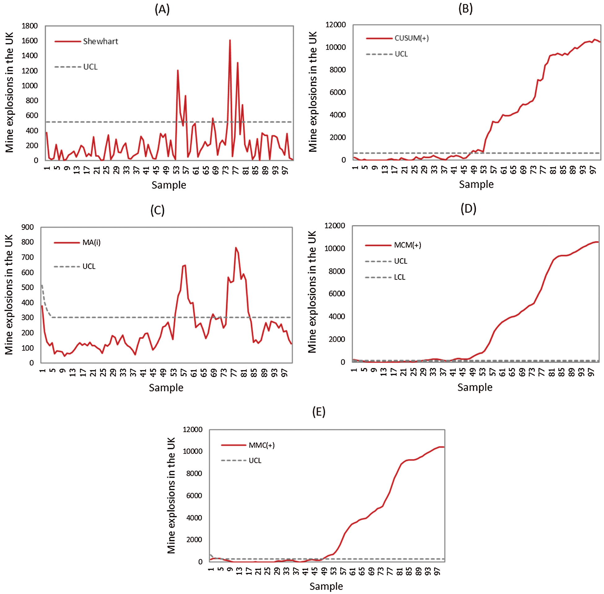
Figure 3: Comparison to detect a change in the mine explosion in the UK from 1875-1951 between Shewhart, CUSUM, MA, CUSUM-MA, and MA-CUSUM control charts, (A) Shewhart chart; (B) CUSUM chart; (C) MA chart; (D) CUSUM-MA chart and (E) MA-CUSUM chart

Acknowledgement: The authors would like to express their gratitude to Mahasarakham University, Thailand, and King Mongkut’s University of Technology North Bangkok, for their promotion and supporting for the scholarship to the researcher.

Funding Statement: Thailand Science Research and Innovation, Ministry of Higher Education, Science, Research. Contract no. KMUTNB-BasicR-64-01.

Conflicts of Interest: The authors declare that they have no conflicts of interest to report regarding the present study.

References

 1.  W. A. Shewhart, “Statistical control,” Economic Control of Quality Manufactured Product, 1st ed., vol. 11. New York, USA: D. Van Nostrand Company, pp. 145, 1931. [Google Scholar]

 2.  E. S. Page, “Continuous inspection schemes,” Biometrika, vol. 41, no. 1-2, pp. 100–115, 1954. [Google Scholar]

 3.  S. W. Roberts, “Control chart tests based on geometric moving average,” Technometrics, vol. 1, no. 3, pp. 239–250, 1959. [Google Scholar]

 4.  B. C. Khoo, “A Moving average control chart for monitoring the fraction non-conforming,” Quality and Reliability Engineering International, vol. 20, no. 6, pp. 617–635, 2004. [Google Scholar]

 5.  N. Abbas, M. Riaz and R. J. M. M. Does, “Mixed exponentially weighted moving average-cumulative sum charts for process monitoring,” Quality and Reliability Engineering International, vol. 29, no. 3, pp. 345–356, 2013. [Google Scholar]

 6.  Q. U. A. Khaliq, M. Riaz and A. Shabbir, “On designing a new Tukey - EWMA control chart for process monitoring,” International Journal of Advanced Manufacturing Technology, vol. 82, no. 1-4, pp. 1–23, 2016. [Google Scholar]

 7.  M. Raiz, Q. U. A. Klaliq and S. Gul, “Mixed Tukey EWMA - CUSUM control chart and its applications,” Quality Technology & Quantitative Management, vol. 14, no. 4, pp. 378–411, 2017. [Google Scholar]

 8.  R. Taboran, S. Sukparungsee and Y. Areepong, “Mixed Moving Average – Exponentially Weighted Moving Average Control Charts for Monitoring of Parameter Change,” in Proc. IMECS 2019, Hong Kong, HK, pp. 411–415, 2019. [Google Scholar]

 9.  P. Phanthuna, Y. Areepong and S. Sukparungsee, “Exact run length evaluation on a two-sided modified exponentially weighted moving average chart for monitoring process mean,” Computer Modeling in Engineering & Sciences, vol. 127, no. 1, pp. 23–41, 2021. [Google Scholar]

10. S. Sukparungsee, Y. Areepong and R. Taboran, “Exponentially weighted moving average - Moving average charts for monitoring the process mean,” PLOS ONE, vol. 15, no. 2, pp. e0228208, 2020. [Google Scholar]

11. B. Zaman, M. Riaz, N. Abbas and R. J. M. M. Does, “Mixed sumulative sum-exponentially weighted moving average control charts: An efficient way of monitoring process location,” Quality and Reliability Engineering International, vol. 31, no. 8, pp. 1407–1421, 2015. [Google Scholar]

12. D. C. Montgomery, “Cumulative sum and exponentially weighted moving average control charts,” Introduction to Statistical Quality Control, 6th ed., vol. 9. New York, USA: John Wiley and Sons, pp. 428, 2009. [Google Scholar]

13. S. Phantu and S. Sukparungsee, “A mixed double exponentially weighted moving average - Tukey’s control chart for monitoring of parameter change,” Thailand Statistician, vol. 18, no. 4, pp. 392–402, 2020. [Google Scholar]

14. F. F. Gan, “An optimal design of cumulative sum control charts based on median run length,” Journal of Statistical Computation and Simulation, vol. 45, no. 3-4, pp. 169–184, 1993. [Google Scholar]

15. F. F. Gan, “An optimal design of EWMA control chart based on median run length,” Journal of Statistical Computation and Simulation, vol. 23, no. 2, pp. 485–503, 1994. [Google Scholar]

16. Y. Wu, “Change-point estimation,” Inference for change-point and post-change means after a CUSUM test, Lecture Notes in Statistics. Vol. 180. New York, USA: Springer, pp. 15–35, 2005. [Google Scholar]

17. R. Taboran, S. Sukparungsee and Y. Areepong, “A new nonparametric Tukey MA-EWMA control charts for detecting mean shifts,” IEEE Access, vol. 8, pp. 207249–207259, 2020. [Google Scholar]

This work is licensed under a Creative Commons Attribution 4.0 International License, which permits unrestricted use, distribution, and reproduction in any medium, provided the original work is properly cited.