DOI:10.32604/iasc.2022.018663
| Intelligent Automation & Soft Computing DOI:10.32604/iasc.2022.018663 | |
| Article |
Energy Saving Control Approach for Trajectory Tracking of Autonomous Mobile Robots
1Department of Mechanical Engineering, National Pingtung University of Science and Technology, Pingtung, 912301, Taiwan
2Department of Systems and Naval Mechatronic Engineering, National Cheng Kung University, Tainan, 701401, Taiwan
3Center for Teacher Education Program, National Pingtung University of Science and Technology, Pingtung, 912301, Taiwan
4Department of Data Science and Big Data Analytics, Providence University, Taichung, 43301, Taiwan
*Corresponding Author: Chiou-Jye Huang. Email: cjh1007@pu.edu.tw
Received: 16 March 2021; Accepted: 26 April 2021
Abstract: This research presents an adaptive energy-saving H2 closed-form control approach to solve the nonlinear trajectory tracking problem of autonomous mobile robots (AMRs). The main contributions of this proposed design are as follows: closed-form approach, simple structure of the control law, easy implementation, and energy savings through trajectory tracking design of the controlled AMRs. It is difficult to mathematically obtained this adaptive H2 closed-form solution of AMRs. Therefore, through a series of mathematical analyses of the trajectory tracking error dynamics of the controlled AMRs, the trajectory tracking problem of AMRs can be transformed directly into a solvable problem, and an adaptive nonlinear optimal controller, which has an extremely simple form and energy-saving properties, can be found. Finally, two test trajectories, namely circular and S-shaped reference trajectories, are adopted to verify the control performance of the proposed adaptive H2 closed-form control approach with respect to an investigated H2 closed-form control design.
Keywords: Energy saving; adaptive H2 closed-form control; trajectory tracking
In recent decades, comprehensive applications of autonomous mobile robots (AMRs) have attracted considerable attention. These AMRs with extended energy endurance, more precise motion ability, and effective control approaches have been applied in the transportation, security, and inspection domains. Thus, a precise motion controller for AMRs and energy saving are becoming increasingly important in the robotics application field, which have been discussed in many studies [1–6]. According to existing studies, it remains difficult to improve the control design when using an extremely simple structure and to realize energy saving in AMRs while accurately and effectively tracking the desired robot trajectory. For trajectory tracking control design, AMRs must be capable of converging the tracking errors of the real trajectory and the desired trajectory as close to zero as possible while considering the influence of modeling uncertainties. A survey of the literature revealed that many studies have focused on the trajectory tracking control of AMRs, for example, trajectory tracking control through backstepping [7–10], sliding mode control [11–14], feedback linearization [15–17], neural networks [18–22], fuzzy control [23–28], and the H2 [29,30] approach. In practice, it is challenging to implement microchip operation and torque output with low energy consumption by using the aforementioned control algorithm methodologies or extremely complex theoretical structures.
For these reasons, an innovative nonlinear energy-saving control approach with a simple control structure that can provide high-performance trajectory tracking for AMRs is presented in this paper. To reduce computational costs and output low-energy torque, a novel energy-saving adaptive H2 closed-form control approach for the trajectory tracking of AMRs is developed. Furthermore, this problem is directly solved using a nonlinear time-varying differential equation. Moreover, the proposed adaptive H2 closed-form solution must satisfy an H2 optimal performance index. In such a circumstance, it is extremely difficult to obtain the solution of a nonlinear time-varying differential equation. However, this solution can be expanded and inferred by selecting suitable state variable transformations and performing mathematical analyses of the dynamic equations of the trajectory tracking error. With such a solution, the adaptive H2 closed-form control approach for the trajectory tracking of AMRs will have a direct implementation structure and provide energy saving.
The remainder of this paper is organized as follows. Section 2 describes the mathematical model of trajectory tracking error of AMRs. In Section 3, the adaptive H2 closed-form controller design for AMR trajectory tracking is described. Section 4 illustrates the simulation results obtained for AMRs by using the proposed approach. Finally, our concluding remarks are given in Section 5.
2 Trajectory Tracking Error Mathematical Model
The trajectory tracking error mathematical model of AMRs is presented in this section. Based on the standard trajectory tracking error mathematical equation and the geometry relationship between the AMR and global coordinate systems, a controlled AMR with a nonlinear trajectory tracking error dynamic equation can be inferred as follows.
In Fig. 1, a schematic of the controlled AMR that has two driving wheels and one omnidirectional wheel is illustrated. The radius of the driving wheels is r. The instantaneous position of the controlled AMR in the system reference frame {O, X, Y} is denoted by p. (
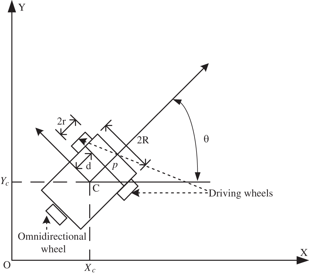
Figure 1: Schematic of the autonomous mobile robot system
Under the nonslipping condition, a standard AMR system usually moves along the orientation of the driving wheels’ axis. Hence, the kinematics of the controlled AMR with constraints can be expressed using the following equation [31]:
where
In this study, the dynamics of the controlled AMR are inferred using the Euler–Lagrange method, as expressed in Eq. (3).
where
Details of the AMR dynamics are as follows:
where
2.2 Trajectory Tracking Error Dynamics of Controlled AMR
Suppose
where
According to Eqs. (3) and (5), the trajectory tracking error dynamics can be described as follows:
Mathematically, it is difficult to use Eq. (5) to solve the trajectory tracking problem of controlled AMRs because of the structure of the error dynamics between the controlled AMR and the desired trajectory. For simplifying the design complexity of this proposed closed-form control approach, a proportional-derivative (PD)-type transformation
where
where
From Eq. (7), the dynamic Eq. (5) of trajectory tracking error can be revised as follows:
where
and
If
then the dynamic equation of trajectory tracking error can be revised as follows:
where
3 Adaptive H2 Closed-From Control Approach Design
3.1 Trajectory Tracking Problem of Adaptive H2 Closed-Form
An analytic adaptive H2 control law for the AMR is deduced from the following equations. To inspect Eq. (11), given the weighting matrices
The aforementioned performance index can be achieved for all
3.2 Adaptive H2 Closed-Form Control Design for AMR
In this section, we solve the AMR trajectory tracking control problem described in Section 2. To this end, we present a novel energy-saving adaptive H2 closed-form control approach for trajectory tracking of the AMR based on the following nonlinear adaptive H2 closed-form control theorem.
Theorem: To obtain the dynamic equation of the trajectory tracking error of the AMR control system described in Eq. (8), the adaptive H2 closed-form control law
where
and
If
It is difficult to determine the adaptive H2 closed-form solution and solve the nonlinear time-varying differential equations in Eqs. (5) and (14). Therefore, this result is a great achievement for the trajectory tracking of AMRs because the adaptive H2 closed-form solution can be directly derived from Eq. (14).
3.3 Adaptive H2 Closed-Form Solution of Nonlinear Time-Varying Differential Equation
In general, it is difficult to solve
Because state-space transformation matrix Eq. (9) has been applied to the control design, the solution
where
To investigate the second and third terms on the left-hand side of time-varying differential Eq. (14), the following equations can be derived using the dynamic equation of trajectory tracking error in Eq. (5) and the selected relationship in Eq. (15):
By using the results of Eqs. (16) and (17), time-varying differential Eq. (14) can be rewritten as the following algebraic equation.
In addition, the optimal control law and adaptive law can be expressed as Eqs. (19) and (20), respectively.
where
where
Using the definitions of
with
Then, the following adaptive H2 control law can be used to solve the trajectory tracking problem of adaptive H2 closed-form control.
where
In this section, a verification scenario with the H2 closed-form and adaptive H2 closed-form control approach for trajectory tracking of a circle and an S shape is presented using the MATLAB software application. According to the aforementioned simulation results, this adaptive H2 closed-form control approach will be certified the performances of trajectory tracking and energy saving of the AMR are more excellent than H2 closed-form control approach.
4.1 Configuration of Simulation Environment
To construct the simulation environment, the following parameters of the practical AMR are employed:
where
Figs. 2–8 show the simulation results of the AMR driven by the H2 closed-form and adaptive H2 closed-form control approaches for tracking a desired circular trajectory with a radius of 3.8 m. The verification results of the H2 closed-form and adaptive H2 closed-form control approaches for tracking this circular trajectory are displayed in Figs. 2 and 3. These results indicate that the trajectory tracking performance of the H2 closed-form and adaptive H2 closed-form control approaches for the desired circular trajectory is adequate. The circular trajectory tracking errors along the x-y axis and angle-to-convergence rates obtained using the H2 closed-form and adaptive H2 closed-form control approach are displayed in Figs. 4–6. The torque performance results of trajectory tracking have outstanding convergence rates that approach zero rather quickly, as indicated in Figs. 7 and 8. Especially, the adaptive H2 closed-form control approach can track the desired circular trajectory of the AMR more rapidly and yield superior trajectory tracking performance and energy savings than the H2 closed-form control approach.
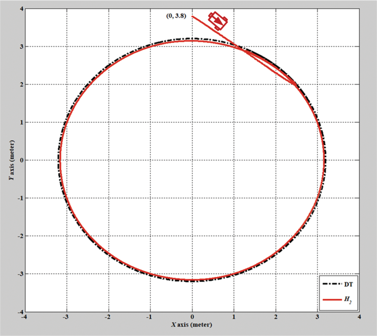
Figure 2: Verification result of H2 closed-form control approach with a circular trajectory from xc = 0 m, yc = 3.8 m
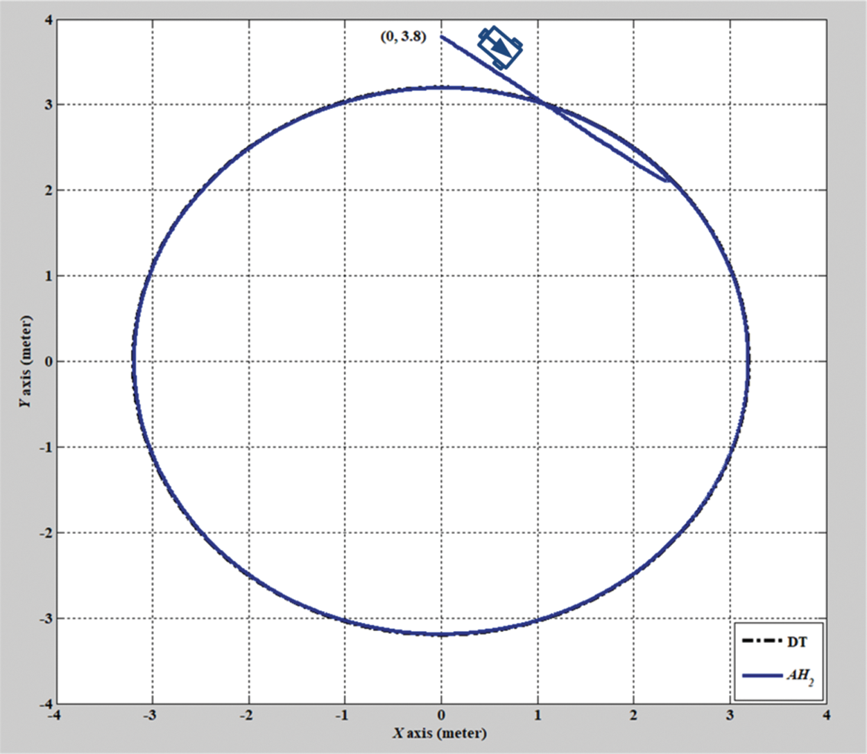
Figure 3: Verification result of the adaptive H2 closed-form control approach with a circular trajectory from xc = 0 m, yc = 3.8 m
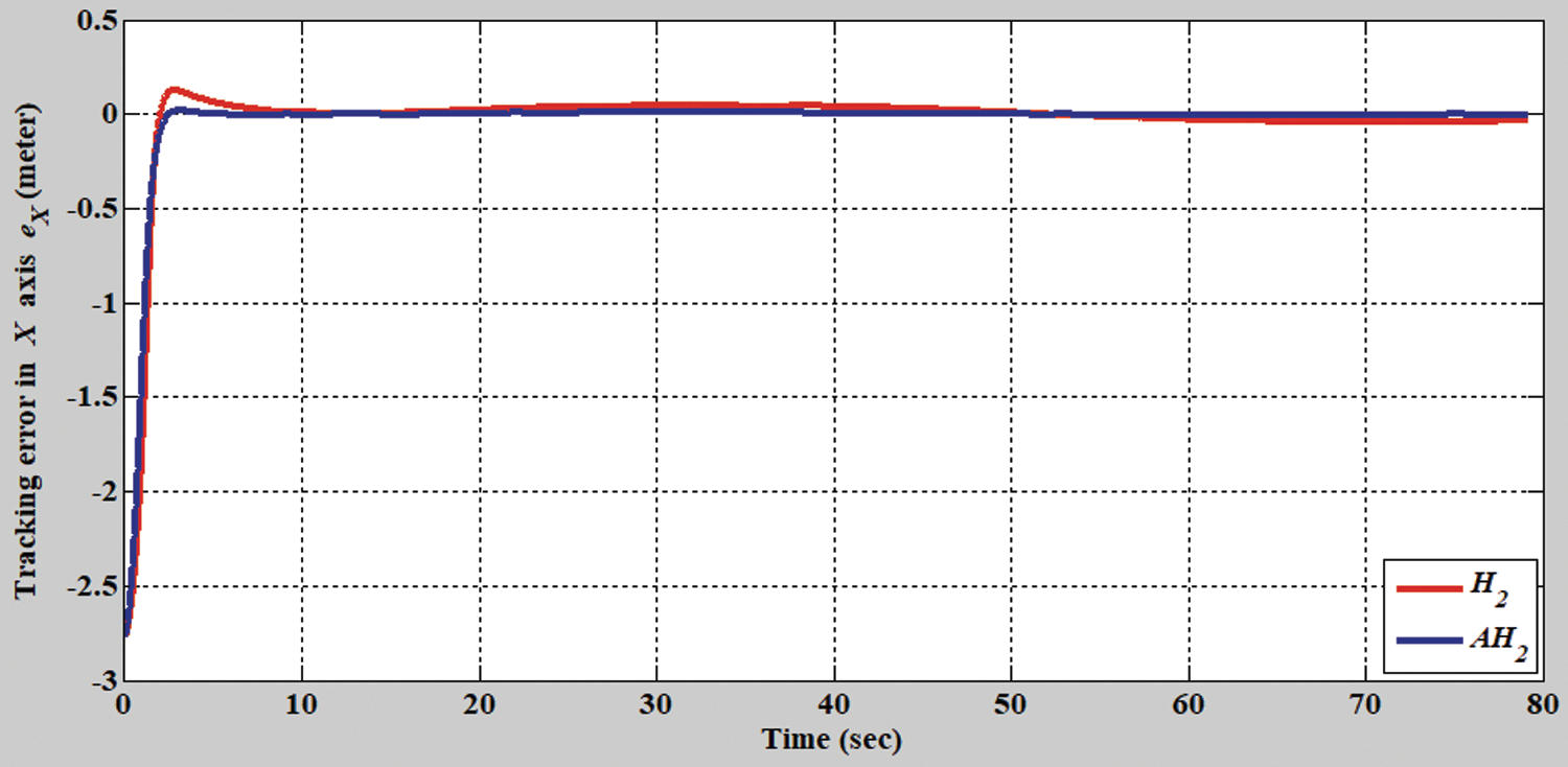
Figure 4: Tracking error results of the H2 closed-form and adaptive H2 closed-form control approaches for the x-axis with a circular trajectory from xc = 0 m, yc = 3.8 m
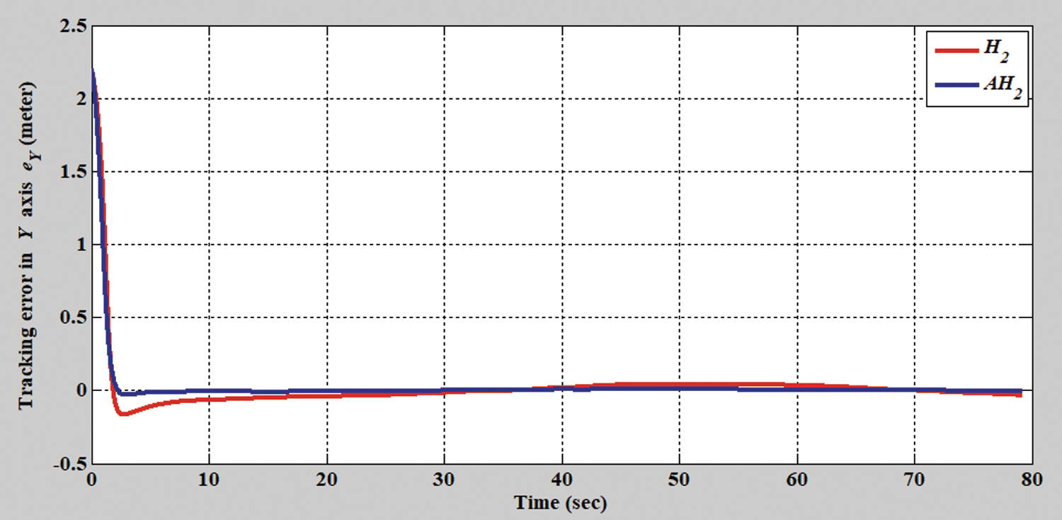
Figure 5: Tracking error results of the H2 closed-form and adaptive H2 closed-form control approaches for the y-axis with a circular trajectory from xc = 0 m, yc = 3.8 m
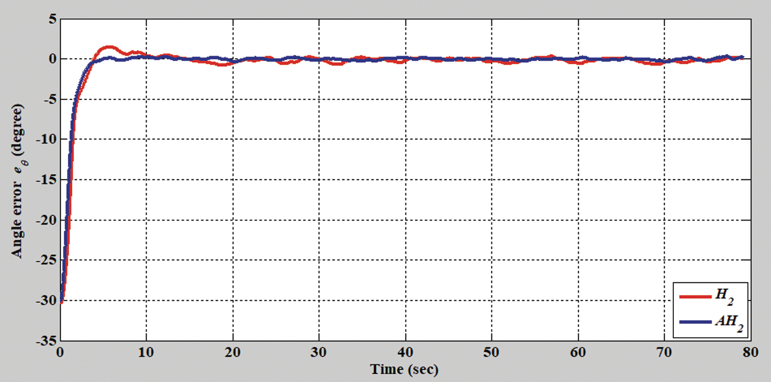
Figure 6: Tracking error results of the H2 closed-form and adaptive H2 closed-form control approaches for angle with a circular trajectory from xc = 0 m, yc = 3.8 m
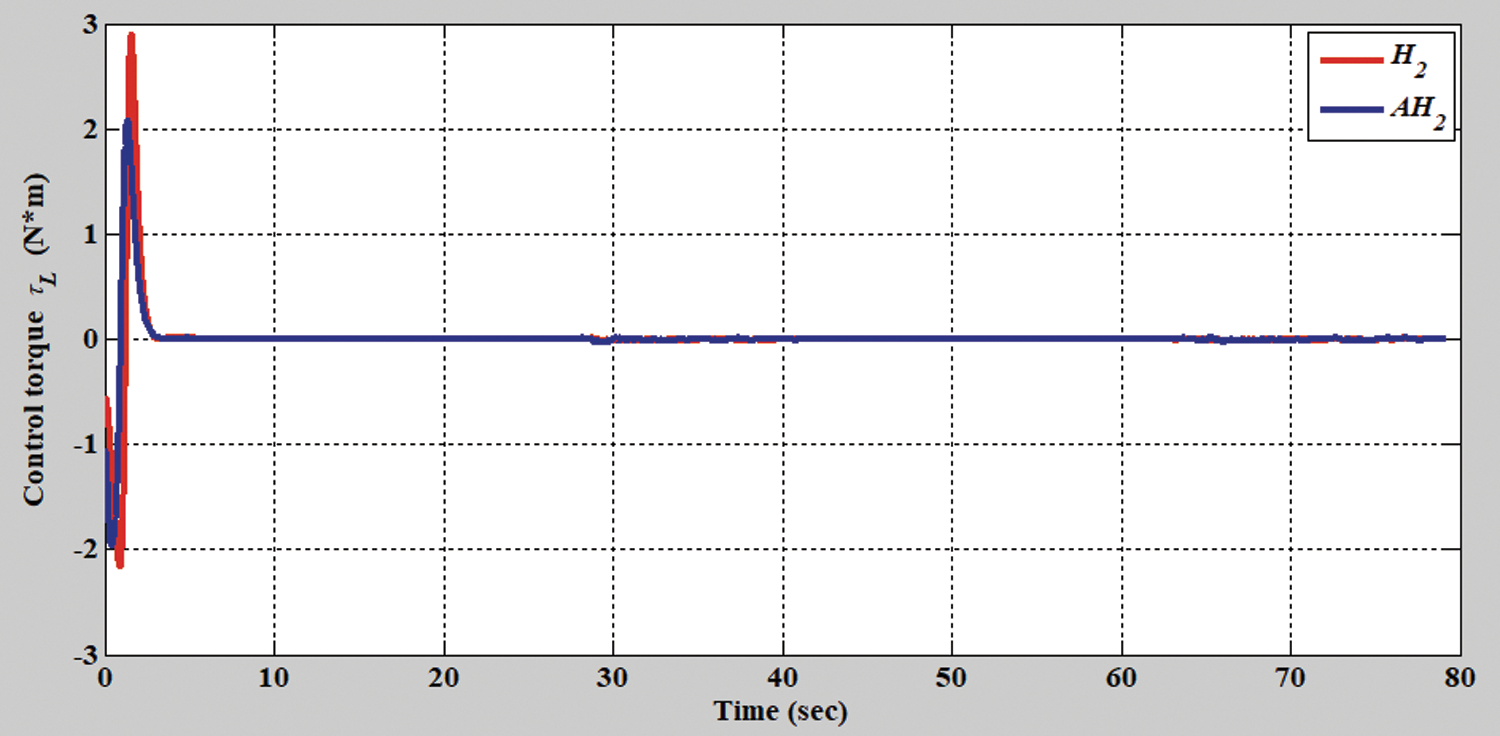
Figure 7: Verification results of the H2 closed-form and adaptive H2 closed-form control approaches for left torque with a circular trajectory from xc = 0 m, yc = 3.8 m
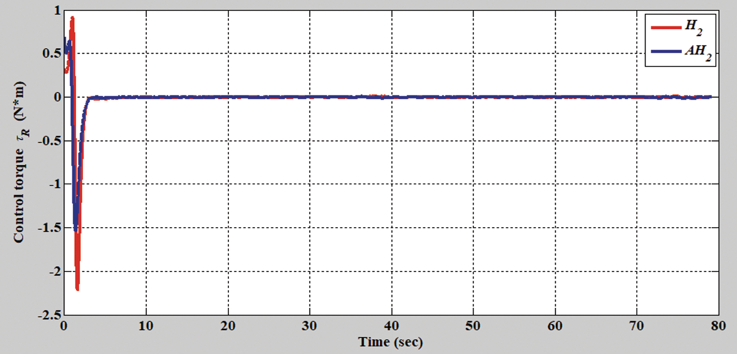
Figure 8: Verification results of the H2 closed-form and adaptive H2 closed-form control approaches for right torque with a circular trajectory from xc = 0 m, yc = 3.8 m
In the second simulation scenario, the verification results of the H2 closed-form and adaptive H2 closed-form control approaches for an S-shaped trajectory with a radius of 3.8 m are displayed in Figs. 9 and 10. The tracking errors of the adaptive H2 closed-form control approach for the desired S-shaped trajectory illustrate an outstanding performance, as displayed in Figs. 11–13. Moreover, the torque performance is notable, as illustrated in Figs. 14 and 15. Finally, the proposed adaptive H2 closed-form control approach can track the desired S-shaped trajectory faster than the H2 closed-form control approach, and the energy-saving effect of the adaptive H2 closed-form control approach is superior to that of the H2 closed-form control design in this simulation scenario.
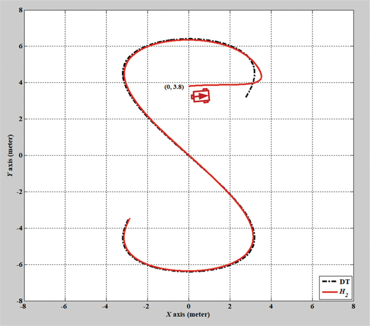
Figure 9: Verification result of H2 closed-form control approach for S-shaped trajectory from xc = 0 m, yc = 3.8 m
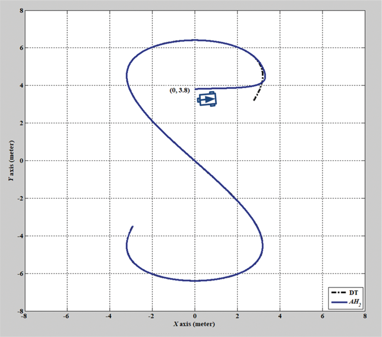
Figure 10: Verification result of adaptive H2 closed-form control approach for S-shaped trajectory from xc = 0 m, yc = 3.8 m
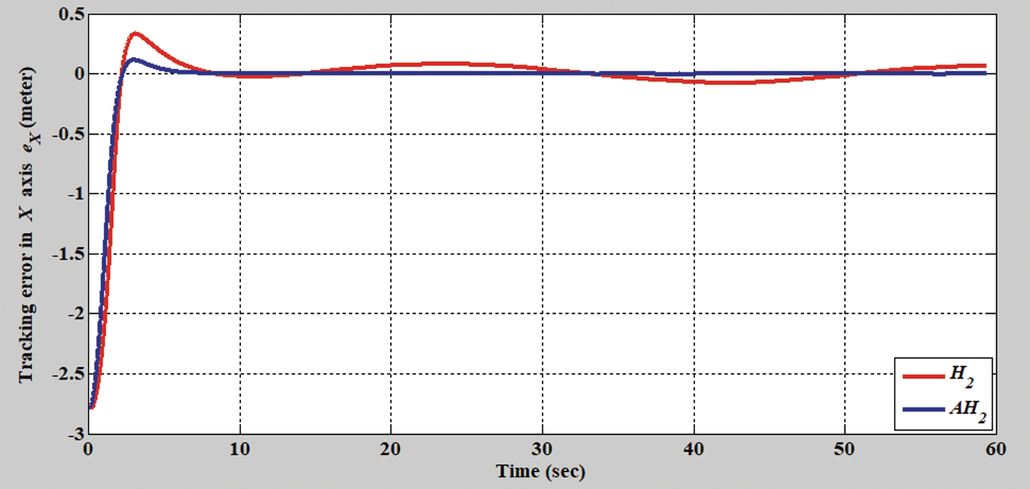
Figure 11: Tracking error of the H2 closed-form and adaptive H2 closed-form control approaches along x-axis for S-shaped trajectory from xc = 0 m, yc = 3.8 m
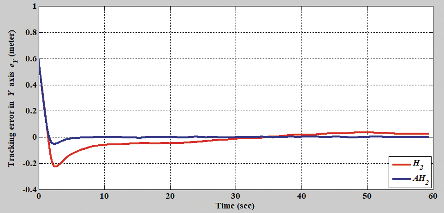
Figure 12: Tracking error of the H2 closed-form and adaptive H2 closed-form control approaches along y-axis for S-shaped trajectory from xc = 0 m, yc = 3.8 m
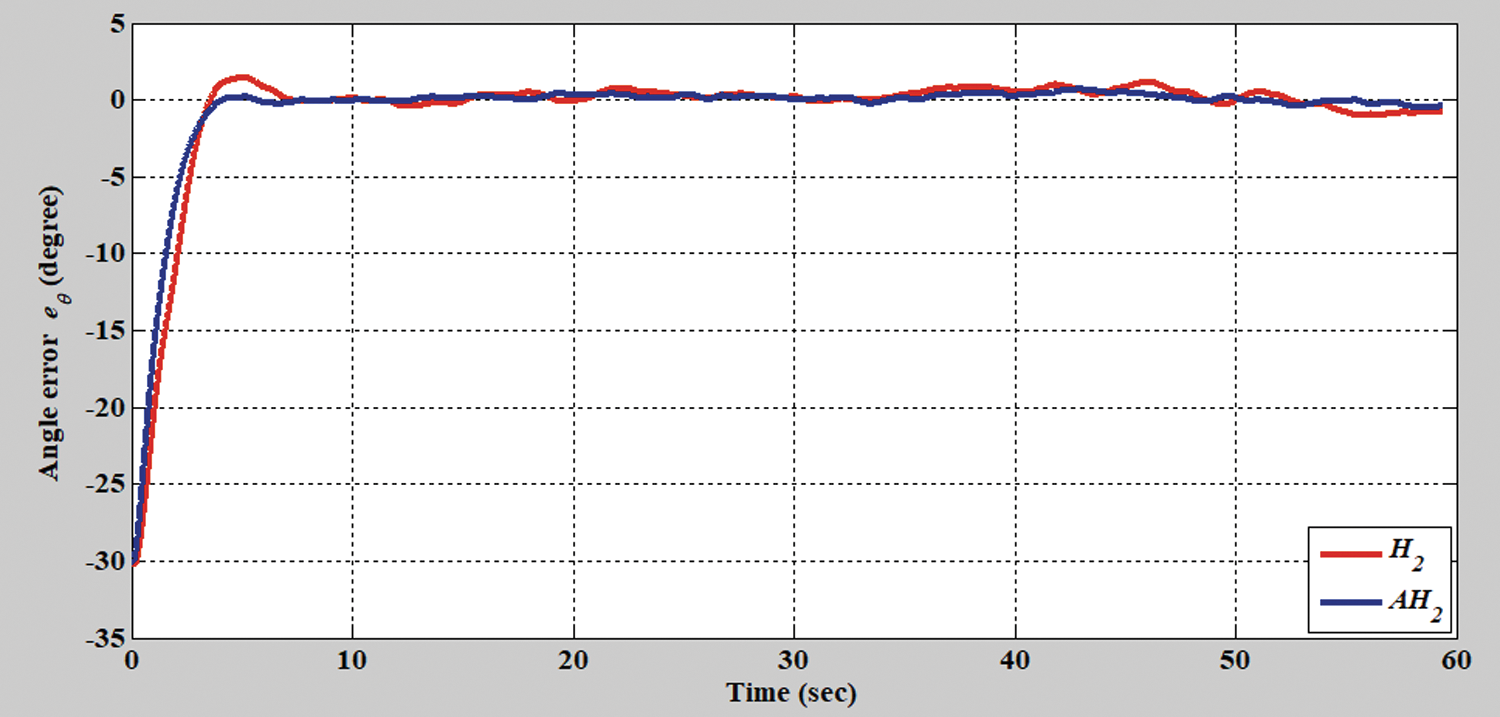
Figure 13: Tracking error of the H2 closed-form and adaptive H2 closed-form control approaches in terms of angle for S-shaped trajectory from xc = 0 m, yc = 3.8 m
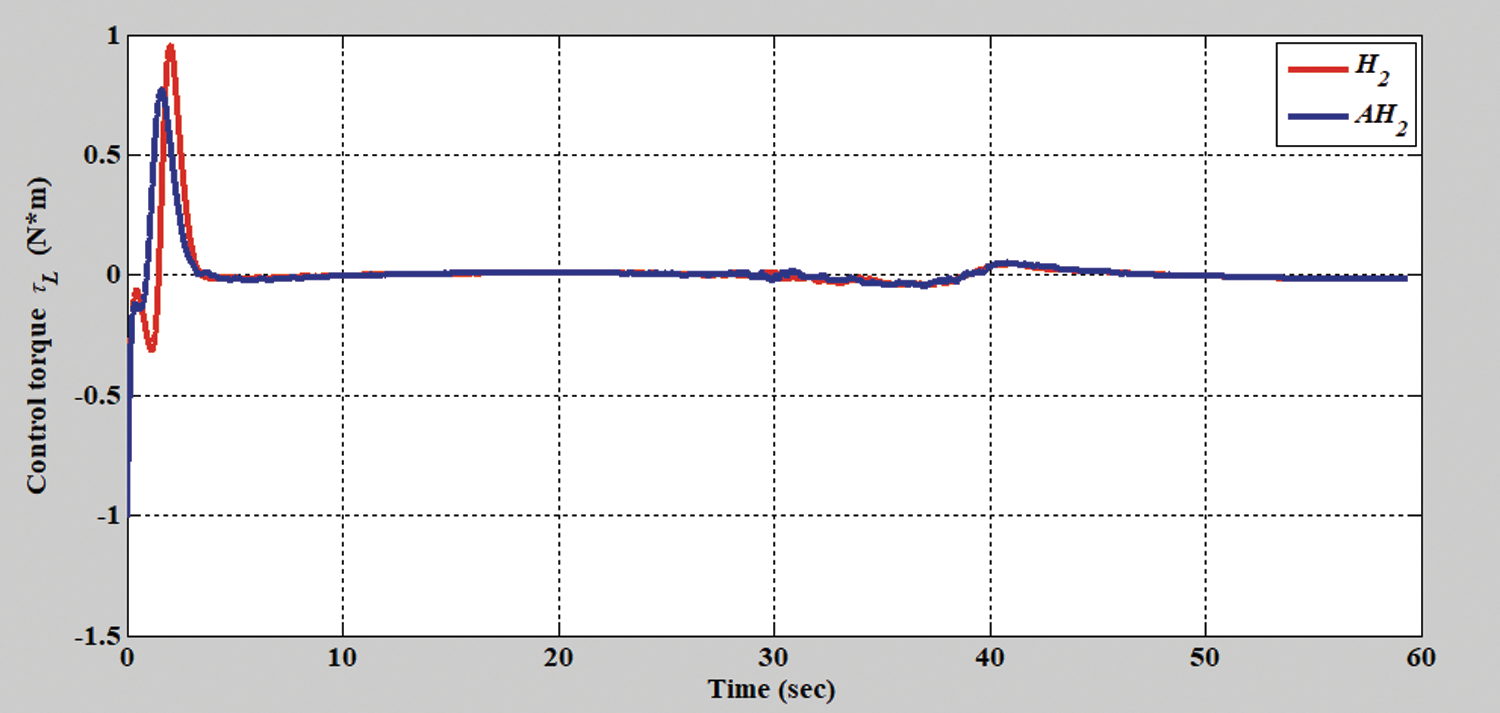
Figure 14: Verification result of the H2 closed-form and adaptive H2 closed-form control approaches in terms of left torque for S-shaped trajectory from xc = 0 m, yc = 3.8 m
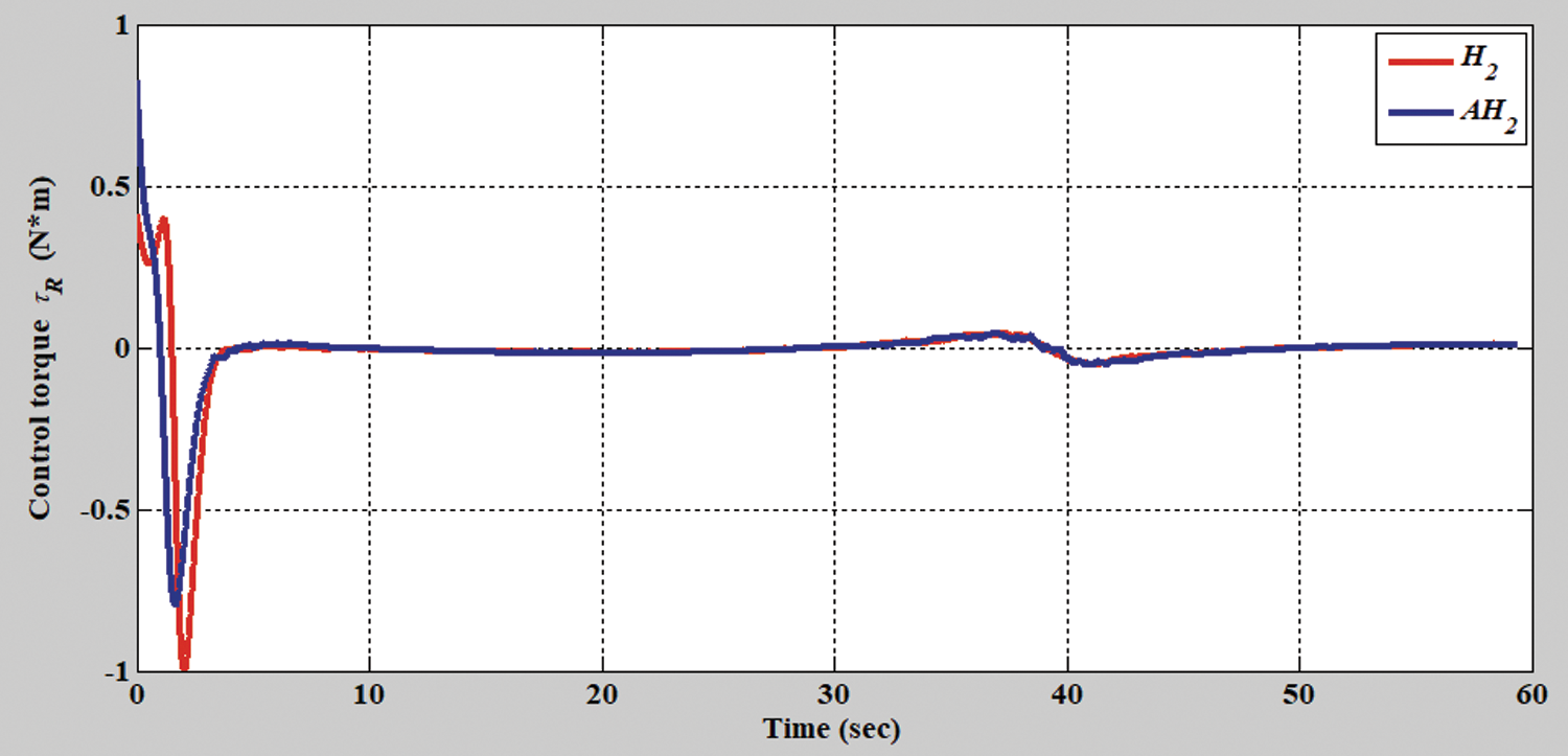
Figure 15: Verification result of H2 closed-form and adaptive H2 closed-form control approaches in terms of right torque for S-shaped trajectory from xc = 0 m, yc = 3.8 m
Suboptimal trajectory tracking designs have been studied for autonomous mobile wheel robots in the past decades, and most of them have achieved acceptable control performance. However, they have disadvantages such as their extremely complex control structures, such as the sliding mode and backstepping control methods. For simultaneously achieving satisfactory tracking performance and a simple control structure, an analytical adaptive nonlinear control scheme was developed to track the trajectory of autonomous mobile wheel robots in this study. The proposed adaptive control design consists of an adaptive cancellation term that is used to cancel the nonlinear component of tracking errors and an optimal control term to minimize the power consumption when tracking the desired trajectories. Thus, the proposed control method has an impressive property; that is, without knowing the system parameters of autonomous mobile wheel robots, the desired trajectory tracking performance can be maintained by exploiting the adaptive learning ability of the proposed method. The simulation results indicate that the proposed adaptive nonlinear control method delivers promising trajectory tracking performance for WMRs because the tracking errors quickly converge to zero when a large amount of modeling uncertainties appear. Therefore, the proposed method has the advantages of being able to execute tasks such as the uploading and downloading of goods and regular patrolling.
Funding Statement: This research was funded by the MOST (Ministry of Science and Technology of Taiwan, project number is MOST 109-2221-E-020-017 -.
Conflicts of Interest: The authors declare that they have no conflicts of interest to report regarding the present study.
1. C. Henkel, A. Bubeck and W. Xu, “Energy efficient dynamic window approach for local path planning in mobile service robotics,” IFAC-Papersonline, vol. 49, no. 15, pp. 32–37, 2016. [Google Scholar]
2. M. Yacoub, D. Necsulescu and J. Sasiadek, “Energy consumption optimization for mobile robots motion using predictive control,” Journal of Intelligent & Robotic Systems, vol. 83, pp. 585–602, 2016. [Google Scholar]
3. S. Mohamed, A. Yamada, S. Sano and N. Uchiyama, “Design of a redundant autonomous drive system for energy saving and fail safe motion,” Advances in Mechanical Engineering, vol. 8, no. 11, pp. 1–15, 2016. [Google Scholar]
4. S. Mohamed, R. Tobias and N. Uchiyama, “Robust control of a redundant autonomous drive system for energy saving and fail safe motion,” Advances in Mechanical Engineering, vol. 9, no. 5, pp. 1–16, 2017. [Google Scholar]
5. G. Carabin, E. Wehrle and R. Vidoni, “A review on energy-saving optimization methods for robotic and automatic systems,” Robotics, vol. 6, no. 4, pp. 1–21, 2017. [Google Scholar]
6. T. Abukhalil, H. Almahafzah, M. Alksasbeh and A. Alqaralleh, “Power optimization in mobile robots using a real-time heuristic,” Journal of Robotics, vol. 21, no. 5, pp. 1–8, 2020. [Google Scholar]
7. Z. Qiang, L. Zengbo and C. Yao, “A back-stepping based trajectory tracking controller for a non-chained nonholonomic spherical robot,” Chinese Journal of Aeronautics, vol. 21, no. 5, pp. 472–480, 2008. [Google Scholar]
8. B. Ibari and L. Benchikh, “Backstepping approach for autonomous mobile robot trajectory tracking,” Indonesian Journal of Electrical Engineering and Computer Science, vol. 2, no. 3, pp. 478–485, 2016. [Google Scholar]
9. J. R. Garcia-Sanchez, S. Tavera-Mosqueda, R. Silva-Ortigoza, V. M. Hernandez-Guzman and J. Sandoval-Gutierrez, “Tracking control for mobile robots considering the dynamics of all their subsystems: Experimental implementation,” Complexity, vol. 2017, no. 4, pp. 1–18, 2017. [Google Scholar]
10. H. Mirzaeinejad and A. M. Shafei, “Modeling and trajectory tracking control of a two-autonomous mobile robot: Gibbs-Appell and prediction-based approaches,” Robotica, vol. 36, no. 10, pp. 1551–1570, 2018. [Google Scholar]
11. R. Wai and L. Chang, “Adaptive stabilizing and tracking control for a nonlinear inverted-pendulum system via sliding-mode technique,” IEEE Transactions on Industrial Electronics, vol. 53, no. 2, pp. 674–692, 2006. [Google Scholar]
12. R. Solea and U. Nunes, “Trajectory planning and sliding-mode control based trajectory-tracking for cybercars,” Integrated Computer Aided Engineering, vol. 13, no. 1, pp. 1–15, 2006. [Google Scholar]
13. J. R. Garcia-Sanchez, S. Tavera-Mosqueda, R. Silva-Ortigoza, V. M. Hernandez-Guzman and J. Sandoval-Gutierrez, “Robust switched tracking control for autonomous mobile robots considering the actuators and drivers,” Sensors, vol. 18, no. 2, pp. 1–21, 2018. [Google Scholar]
14. G. Wang, C. Zhou, Y. Yu and X. Liu, “Adaptive sliding mode trajectory tracking control for AMR considering skidding and slipping via extended state observer,” Energies, vol. 12, no. 7, pp. 1–16, 2019. [Google Scholar]
15. S. Bharadwaj, A. V. Rao and K. D. Mease, “Entry trajectory tracking law via feedback linearization,” Journal of Guidance, Control, and Dynamics, vol. 21, no. 5, pp. 276–732, 1998. [Google Scholar]
16. A. Kabanov, “Feedback linearized trajectory-tracking control of a mobile robot,” MATEC Web of Conferences, vol. 129, no. 6, pp. 1–4, 2017. [Google Scholar]
17. T. Taniguchi and M. Sugeno, “Trajectory tracking controls for non-holonomic systems using dynamic feedback linearization based on piecewise multi-linear models,” International Journal of Applied Mathematics, vol. 47, no. 3, pp. 1–13, 2017. [Google Scholar]
18. J. Velagic, N. Osmic and B. Lacevic, “Neural network controller for mobile robot motion control,” International Journal of Intelligent Systems and Technologies, vol. 3, no. 3, pp. 1–17, 2018. [Google Scholar]
19. S. Tang and C. K. Ang, “Predicting the motion of a robot manipulator with unknown trajectories based on an artificial neural network,” International Journal Advanced Robotic Systems, vol. 11, pp. 1–9, 2014. [Google Scholar]
20. W. Zheng, H. B. Wang, Z. M. Zhang, N. Li and P. H. Yin, “Multi-layer feed-forward neural network deep learning control with hybrid position and virtual-force algorithm for mobile robot obstacle avoidance,” International Journal of Control, Automation and Systems, vol. 17, no. 4, pp. 1007–1018, 2019. [Google Scholar]
21. P. Bozek, Y. L. Karavaev, A. A. Ardentov and K. S. Yefremov, “Neural network control of a wheeled mobile robot based on optimal trajectories,” International Journal of Advanced Robotic Systems, vol. 1, pp. 1–10, 2020. [Google Scholar]
22. D. Wang, W. Wei, Y. Yeboah, Y. Li and Y. Gao, “A robust model predictive control strategy for trajectory tracking of omni-directional mobile robots,” Journal of Intelligent & Robotic Systems, vol. 98, pp. 439–453, 2020. [Google Scholar]
23. T. F. Wu, “Tracking control of autonomous mobile robots using fuzzy CMAC neural networks,” Journal of Internet Technology, vol. 19, no. 6, pp. 1853–1869, 2018. [Google Scholar]
24. Y. H. Chen and T. H. S. Li, “A novel fuzzy control law for nonholonomic mobile robots,” International Journal of Computational Intelligence in Control, vol. 10, no. 2, pp. 53–59, 2018. [Google Scholar]
25. D. K. Tiep, K. Lee, D. Y. Im, B. Kwak and Y. J. Ryoo, “Design of fuzzy-PID controller for path tracking of mobile robot with differential drive,” International Journal of Fuzzy Logic and Intelligent Systems, vol. 18, no. 32, pp. 220–228, 2018. [Google Scholar]
26. N. Hacene and B. Mendil, “Fuzzy behavior-based control of three autonomous omnidirectional mobile robot,” International Journal of Automation and Computing, vol. 16, pp. 163–185, 2019. [Google Scholar]
27. M. Abdelwahab and V. Parque, “Trajectory tracking of autonomous mobile robots using z-number based fuzzy logic,” IEEE Access, vol. 8, pp. 18426–18441, 2020. [Google Scholar]
28. Y. H. Chen, “A novel fuzzy trajectory tracking control design for autonomous mobile robot,” Advances in Robotics & Mechanical Engineering, vol. 2, no. 3, pp. 142–144, 2020. [Google Scholar]
29. Y. H. Chen, T. H. S. Li and Y. Y. Chen, “A novel nonlinear control law with trajectory tracking capability for mobile robots: Closed-form solution design,” Applied Mathematics and Information Sciences, vol. 7, no. 2, pp. 749–754, 2013. [Google Scholar]
30. Y. H. Chen and S. J. Lou, “Control design of a swarm of intelligent robots: A closed-form H2 nonlinear control approach,” Applied Sciences, vol. 10, no. 3, pp. 1–18, 2020. [Google Scholar]
31. Y. Y. Chen, Y. H. Chen and C. Y. Huang, “Autonomous mobile robot design with robustness properties,” Advances in Mechanical Engineering, vol. 10, no. 1, pp. 1–11, 2018. [Google Scholar]
32. K. Zhou, K. Glover, B. Bodenheimer and J. Doyle, “Mixed H2 and H∞ performance objectives I: Robust performance analysis,” IEEE Transactions Automation Control, vol. 39, no. 8, pp. 1564–1574, 1994. [Google Scholar]
 | This work is licensed under a Creative Commons Attribution 4.0 International License, which permits unrestricted use, distribution, and reproduction in any medium, provided the original work is properly cited. |