Intelligent Automation & Soft Computing DOI:10.32604/iasc.2021.019164
Article

Computational Methods for Non-Linear Equations with Some Real-World Applications and Their Graphical Analysis

Amir Naseem1, M.A. Rehman1 and Thabet Abdeljawad2,3,4,*

1Department of Mathematics, University of Management and Technology, Lahore, Pakistan
2Department of Mathematics and General Sciences, Prince Sultan University, Riyadh, 11586, Saudi Arabia
3Department of Medical Research, China Medical University Hospital, China Medical University, Taichung, 40402, Taiwan
4Department of Computer Science and Information Engineering, Asia University, Taichung, 41354, Taiwan
*Corresponding Author: Thabet Abdeljawad. Email: tabdeljawad@psu.edu.sa
Received: 03 April 2021; Accepted: 04 May 2021

Abstract: In this article, we propose some novel computational methods in the form of iteration schemes for computing the roots of non-linear scalar equations in a new way. The construction of these iteration schemes is purely based on exponential series expansion. The convergence criterion of the suggested schemes is also given and certified that the newly developed iteration schemes possess quartic convergence order. To analyze the suggested schemes numerically, several test examples have been given and then solved. These examples also include some real-world problems such as van der Wall’s equation, Plank’s radiation law and kinetic problem equation whose numerical results showing the better performance, applicability and efficiency of these iteration schemes against the other similar-nature two-step iteration schemes in the literature. Finally, a detailed graphical analysis of the suggested iteration schemes has been given in the form of polynomiographs for the different complex polynomials with the aid of computer technology that reveals the convergence characteristics and other dynamical features of the presented iteration schemes.

Keywords: Non-linear equations; Newton’s method; Ostrowski’s method; Traub’s method; polynomiography

1  Introduction

The polynomial’s root-finding task has played a major role in the entire history of computational and applied mathematics and covers many other fields of modern sciences. In many branches of Engineering, there exist a plethora of problems that can be easily converted to the form of non-linear functions using different mathematical tools and then can be solved through different numerical methods. Analytical methods for these problems are mostly unable to obtain the required solution and ultimately, we have to move towards the different iteration schemes for getting the approximate solution of the given problem. The first and the most important step in an iteration scheme is the selection of the initial guess to execute the algorithm. The main characteristics of an iteration scheme such as rate and order of convergence are mostly depended upon the choice of that starting point. At each step of the iteration scheme, this starting point has been filtered till the required stopping criterion is achieved. Some of the most famous and classical iteration schemes are given in the literature [1–8] and the references therein. The most famous and classical iteration scheme was introduced by Newton [1] in 15th century. With the passage of time, a significant number of scholars researched on the iteration schemes and introduced many modified forms of Newton’s algorithm with higher convergence order. Among them, there are plenty of iteration schemes that involve predictor and corrector steps and usually known as multi-step iterative methods. For further details, see [9–16] and the references therein. Usually, the convergence orders of the multi-step iterative methods are greater due to the involvement of predictor and corrector steps but it causes to increase in the computational cost per iteration because these methods require the evaluation of the function along with the higher-order derivatives which is the main drawback of these methods. It is really a difficult task to manage the convergence rate and the computational cost because it looks that these two quantities are in an inverse relation.

In the last few years, the mathematicians focussed on the above-described issue and tried to modify the existing iteration schemes with low computational cost per iterations and higher convergence rate by implementing several mathematical techniques. In 2007, Noor et al. [17], proposed a sixth-order predictor-corrector type Halley’s method and then made it second-derivative free via finite difference scheme and obtained a novel fifth-order algorithm. In 2017, Rhee et al. [18] developed a new class of three-step optimal eighth-order methods with higher-order weight functions employed in the second and third sub-steps and then investigated their dynamics underlying the purely imaginary extraneous fixed points. Based on the weight combination of midpoint with Simpson quadrature formulae and using the predictor-corrector technique, Hafiz et al. [19] introduced two novel seventh- and ninth-order root-finding algorithms. In 2018, Salimi et al. [20] proposed an optimal class of eighth-order methods with the help of weight functions and the Newton interpolation technique. After that, Solaiman et al. [21] suggested some higher-order optimal methods and proved their applicability by solving some real-life problems in chemical engineering. Very recently, Chu et al. [22] constructed an efficient family of simultaneous iterative methods and give a detailed dynamical analysis of the suggested methods. Some latest work that includes the system of non-linear equations and its relevant fields along with the applications has been given in [23–34] and the references are therein.

In this research article, we give a new idea to derive some new computational methods in the form of iteration schemes. The main idea behind the construction of these schemes is the expansion of exponential series up to fifth term. We also certify that the suggested schemes are quartic-order and then applied to different arbitrary test problems along with some real-world problems for showing its applicability, validity, and accuracy among the other similar-nature two-step iteration schemes in the literature.

2  General Iteration Scheme Based on Exponential Series Expansion

The general iteration scheme based on the expansion of exponential series is given as:

ui+1=vie(−ψ(vi)viψ′(vi)), (1)

With the help of the above general iteration scheme, we will deduce some new algorithms by expanding the exponential series up to two, three, four and five terms.

Expanding Eq. (1) upto two terms gives us the following iterative scheme:

which is actually the well-known fourth-order Traub’s algorithms [12] for computing approximate roots of the non-linear scalar equations.

Again expanding Eq. (1) up to three, four and five terms, we obtain the iterative schemes given as:

which are quite new iteration forms and allow us to suggest the following algorithms.

Algorithm 1

For a given u0 , compute the approximate solution ui+1 by the following iterative schemes:

Algorithm 2

For a given u0 , compute the approximate solution ui+1 by the following iterative schemes:

Algorithm 3

Which are two-step iterative schemes for computing the roots of non-linear scalar equations. One of the most important and basic characteristics of the suggested algorithms is that they are second-derivative free and easy to apply upon those scalar functions whose second derivative does not exist at all. In this sense, the computational cost of these presented algorithms is less that may cause to aquire higher efficiency index.

3  Convergence Analysis

In this section, we will find the convergence order of general iteration scheme given in Eq. (1).

Theorem 1

Suppose that α is a root of the equation ψ(u)=0 . If ψ(u) is sufficiently smooth in the neighborhood of α , then the order of convergence of the general iteration scheme given in Eq. (1) is at least four.

Proof

To analyze the convergence criterion of the iteration scheme Eq. (1), we assume that α is a root of the equation ψ(u)=0 and ei be the error at i th iteration, then ei=ui−α and by using Taylor’s series expansion, we have

ψ(ui)=ψ′(α)[ei+d2ei2+d3ei3+d4ei4+d5ei5+d6ei6+O(ei7)] (2)

where

ψ′(ui)=ψ′(α)[1+2d2ei+3d3ei2+4d4ei3+5d5ei4+6d6ei5+7d7ei6+O(ei7)] (3)

With the help of Eqs. (2) and (3), we get:

vi=α+d2ei2+2(d3−d22)ei3+(3d4−7d3d2+4d23)ei4+(−6d33+20d3d22−10d2d4+4d5−8d24)ei5+(−17d3d4+28d4d22−13d2d5+5d6+33d2d33−52d3d23+16d25)ei6+O(ei7) (4)

ψ(vi)=ψ′(α)[d2ei2+(2d3−2d22)ei3+(5d23−7d2d3+3d4)ei4+(24d3d22−12d24−10d2d4+4d5−6d32)ei5+(−73d3d23+34d4d22+28d25+37d2d32−17d4d3−13d2d5+5d6)ei6+O(ei7)] (5)

ψ′(vi)=ψ′(α)[1+2d22ei2+(4d2d3−4d23)ei3+(6d2d4−11d3d22+8d24)ei4+28d3d23−20d4d22+8d2d5−16d25)ei5+(−16d4d2d3−68d3d24+12d33+60d4d23−26d5d22+10d2d6+32d26)ei6+O(ei7)] (6)

Using Eqs. (4)–(6) in the general iteraion scheme Eq. (1), we arrive at the following equality:

which implies that

The above equation shows that the order of convergence of the general iteration scheme Eq. (1) is at least four and all the algorithms derived from it must possess the same convergence order.

4  Numerical Comparison and Applications

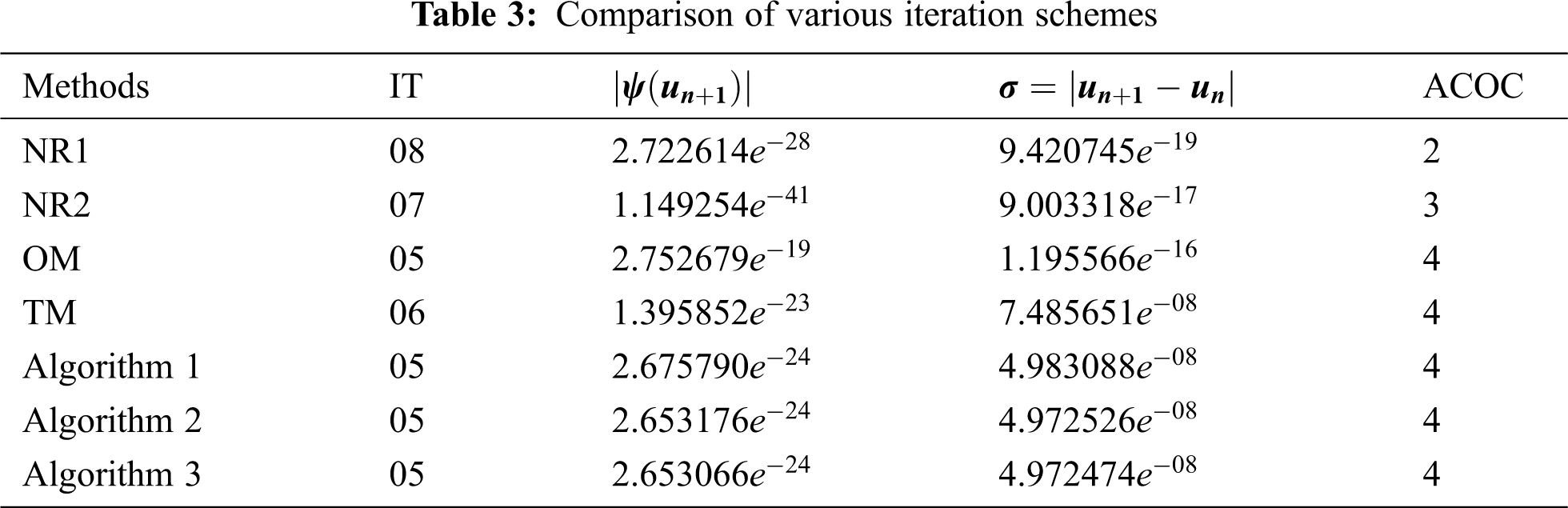
In this section, we include three real-world problems and five arbitrary problems in the form of transcendental and algebraic equations to illustrate the validity, applicability, and efficiency of the newly developed iteration schemes. We compare these iteration schemes with Noor’s method one (NR1) [10], Noor’s method two (NR2) [10], Ostrowski’s Method (OM) [11] and Traub’s method (TM) [12]. For this purpose, we consider the following examples.

4.1 Van Der Wall’s Equation

In Chemical Engineering, the van der Waal’s equation has been used for interpreting real and ideal gas behaviour [35], having the following form:

By taking the specific values of the parameters of the above equation, we can easily convert it to the following non-linear function:

where s represents the volume that can easily be found by solving the function ψ2 . Since the degree of the polynomial is three, so it must possess three roots. Among these roots, there is only one positive real root 1.92984624284786221850 which is feasible because the volume of the gas can never be negative. We start the iteration process with the initial guess x0=1.0 and their results can be seen in Tab. 1.

4.2 Plank’s Radiation Law

In mathematical physics, the Planck’s radiation law [36] is used to calculate the energy density inside an isothermal black body and have the following mathematical form:

Suppose we are interested to find the wavelength γ1 corresponding to the maximum value of the energy density φ(γ1) . To convert the above problem in the form of a non-linear function, we take x=PcγTk and has the following non-linear equation:

One of the approximated roots of the above function is 4.96511423174427630370 that represents the peak value of the wavelength of the radiation. We choose the initial guess x0=6.0 to start the iteration process and the corresponding results through different iteration schemes are given in Tab. 2.

4.3 Kinetic Problem Equation

In Physics, the mathematical form of the equation of kinetic problem is:

where T in the above equality denotes the temperature of the system which is being considered. The above equality was derived from a stirred reactor with cooling coils [37]. By assuming the T=x, the above equality can be converted to the following form:

The above given equation can be utilized to determine the temperature of the system which is being considered. One of the roots of the above equation is 551.77382493032659964000 . To execute the iteration process, we take the starting point x0=500.0 and the corresponding results are given in Tab. 3.

4.4 Transcendental and Algebraic Equations

To numerically analyze the suggested iteration schemes, we consider the following five algebraic and transcendental equations:

as shown in the following Tabs. 4–8.

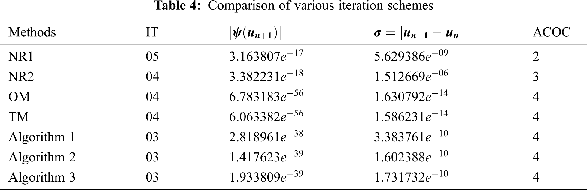
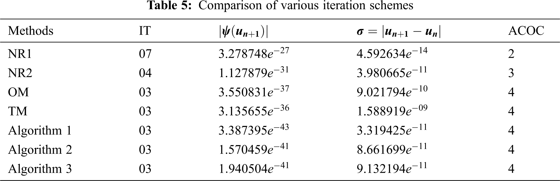
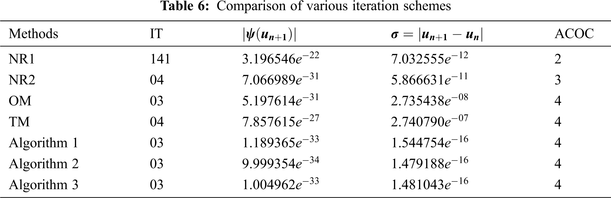
Here, we take Ԑ=10−15 in the following stopping criteria | un+1−un | < Ԑ . The numerical examples have been solved using the computer program Maple 13.

Tabs. 1–8 show the numerical comparisons of the developed iteration schemes with Noor's method one (NR1), Noor's method two (NR2), Ostrowski's method (OM), and Traub's method (TM). In the columns of the given tables, IT denotes the consumption of iterations by each method, |ψ(u)| denotes the absolute value of ψ(u) , un+1 shows the approximate root, σ represents the absolute difference of the consecutive approximations un+1 and un and ACOC stands for the approximate computational order of convergence given as:

That was introduced by Weerakoon et al. [38].

5  Graphical Analysis

This section includes the graphical comparison of the suggested two-step algorithms with the other similar-nature algorithms via polynomiographs for different complex polynomials. A polynomiograph is actually a particular image that has been created in the process of polynomiography, first introduced by Kalantri in 2005 [39]. He defined this term as “the art and science of visualization in the approximation of the zeros of complex polynomials, via fractal and non-fractal images generated through the mathematical convergence properties of iteration functions” [40]. The word “fractal” appeared in the above definition is actually a geometrical image who’s each and every part possesses the same statistical character as the entire, introduced by Mandelbrot [41]. The polynomiographs and fractals, both can be achieved through a variety of numerical algorithms. The polynomiographs and fractals are quite different from each other in terms of structure scale. The “polynomiographer” can modulate the structure and pattern systematically using different numerical algorithms, applied to a variety of complex polynomials. Generally, the polynomiographs and fractals are members of distinct families of graphical objects.

To generate polynomiographs using computer program through different numerical algorithms, we have to choose an initial rectangle R , containing the zeros of the considered complex polynomial. Then corresponding to each point w0 in the region, we run an iterative process and then color the point corresponding to w0 depended upon the approximate convergence of truncated orbit to a root, or lack thereof. The resolution of the generated image relies on the discretization of the rectangle R . For example, if we discretize R into a 2000 by 2000 grid then the result will be a high-resolution image.

Usually, polynomiographs’ colors are purely associated with the iterations needed to approximate the zeros of the complex polynomial with given accuracy and a chosen numerical algorithm. The general and base algorithm for the generation of polynomiograph is presented in the following Algorithm 4.

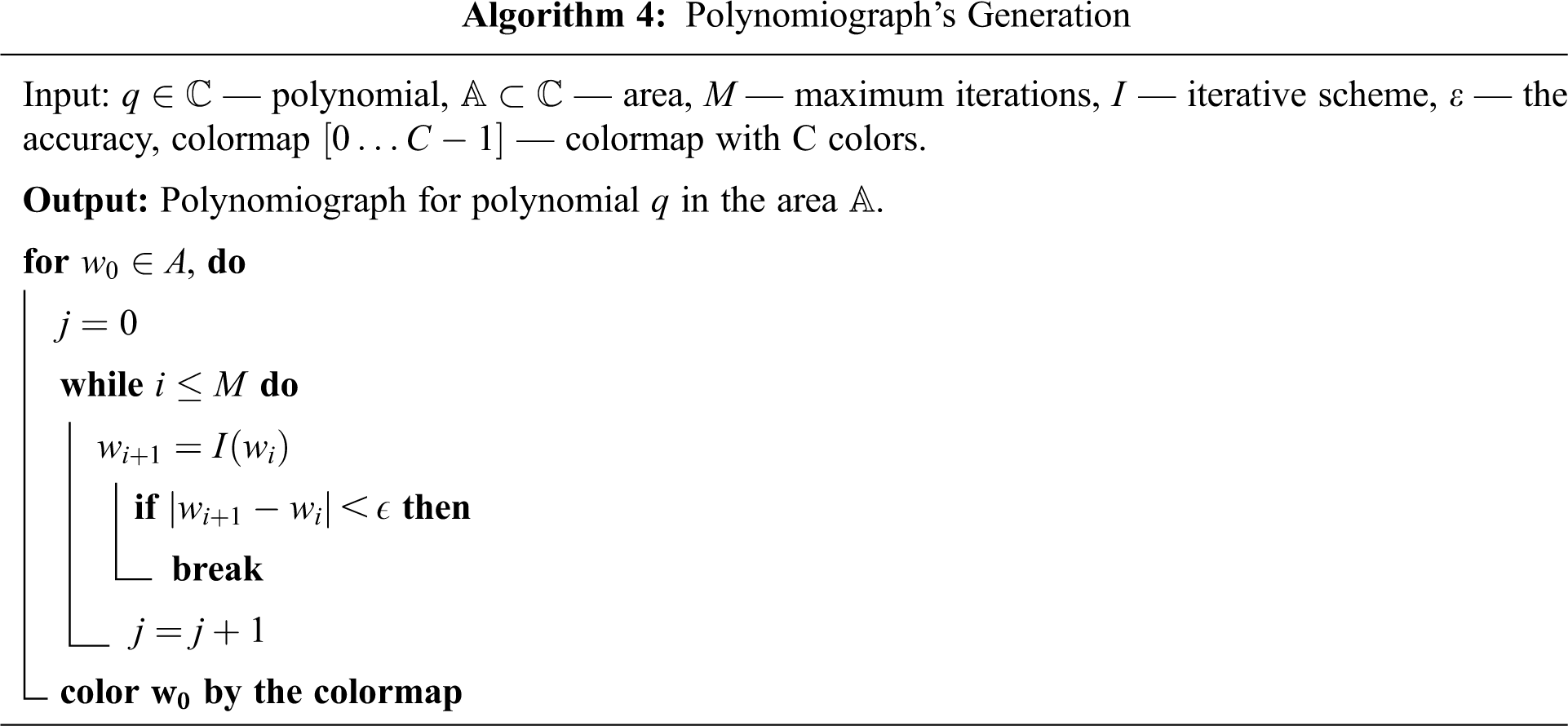
In an iteration scheme that involves the repetition of steps, there always exists a need for the stopping criterion that provides us the information about the convergence or divergence of the considered iteration scheme. Such a test is called a convergence test with the following standard form:

|wi+1−wi|<Ԑ (7)

where wi+1 and wi are the successive iterations in the process and > 0 denotes the accuracy. The convergence test ( wi+1,wi,?) returns TRUE if the considered iteration scheme converged and FALSE in case of divergence. In this paper, we also use the above-described stopping criterion Eq. (7). The different colors of the polynomiograph rely on the consumption of iterations to approximate the root with given accuracy Ԑ . Infinitely many aesthetically pleasing and nice-looking graphical objects can be generated by changing parameter M , where M denotes the upper limit of the number of iterations. The detailed and comprehensive study of polynomiography and its artistic applications are described in Refs. [42–48].

Here we present some particular examples of the following complex polynomials using the proposed iteration schemes and compared them with the polynomiographs obtained by using other similar-nature two-step iteration schemes.

The colormap used for the coloring of iterations in the generation of polynomiographs is presented in the following Fig. 1:

Figure 1: The colormap used for generating polynomiographs

5.1 Polynomiographs for the Polynomial q1(w) Using Various Iterative Methods

In the first experiment, we take the cubic polynomial q1(w)=w3−1, having three distinct roots 1, −12+32i , and −12−32i . To obtain the simple roots of the considered polynomial, we executed all the algorithms through the computer program and the results in the form of the polynomiographs are given in Fig. 2.

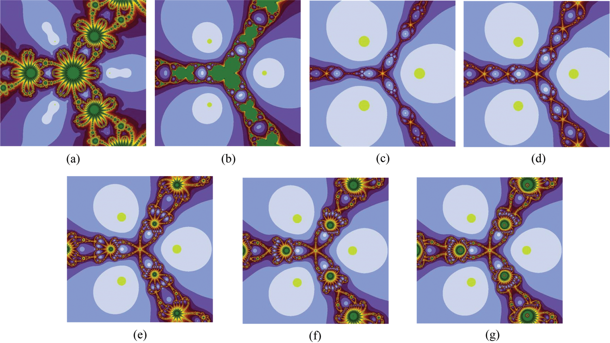
Figure 2: Polynomiographs associated with the polynomial q1(w) . (a) stands for Noor’s method one, (b) stands for Noor’s method two (c) stands for Ostrowski’s method, (d) stands for Traub’s method, (e), (f) and (g) stand for Algorithms 1-3 respectively

5.2 Polynomiographs for the Polynomial q2(w) Using Various Iterative Methods

In the second experiment, we consider the sextic polynomial q2(w)=(w3−1)2, having the same three distinct zeros as the previous polynomial q1(w) but the multiplicity of these zeros is two. To acquire the simple zeros for the considered polynomial, we ran all the algorithms and the corresponding results are shown in Fig. 3.

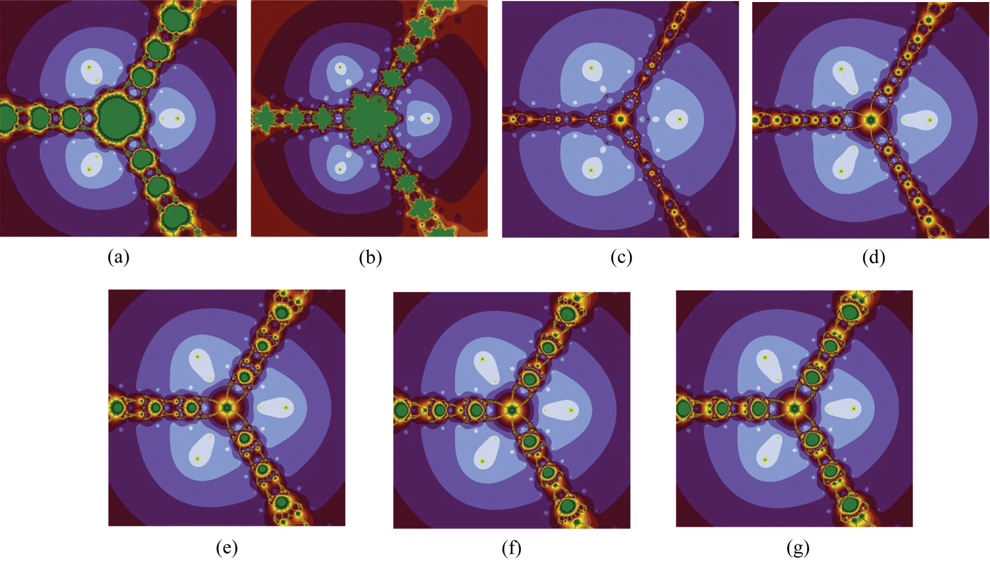
Figure 3: Polynomiographs associated with the polynomial q2(w) . (a) stands for Noor’s method one, (b) stands for Noor’s method two (c) stands for Ostrowski’s method, (d) stands for Traub’s method, (e), (f) and (g) stand for Algorithms 1–3 respectively

5.3 Polynomiographs for the Polynomial q3(w) Using Various Iterative Methods

In the third example, we take the quartic polynomial q3(w)=w4−1, that possesses exactly four simple zeros 1,−1,i,and−i. We generated the graphical objects through the execution of all the algorithms and the results can be seen in the following Fig. 4.

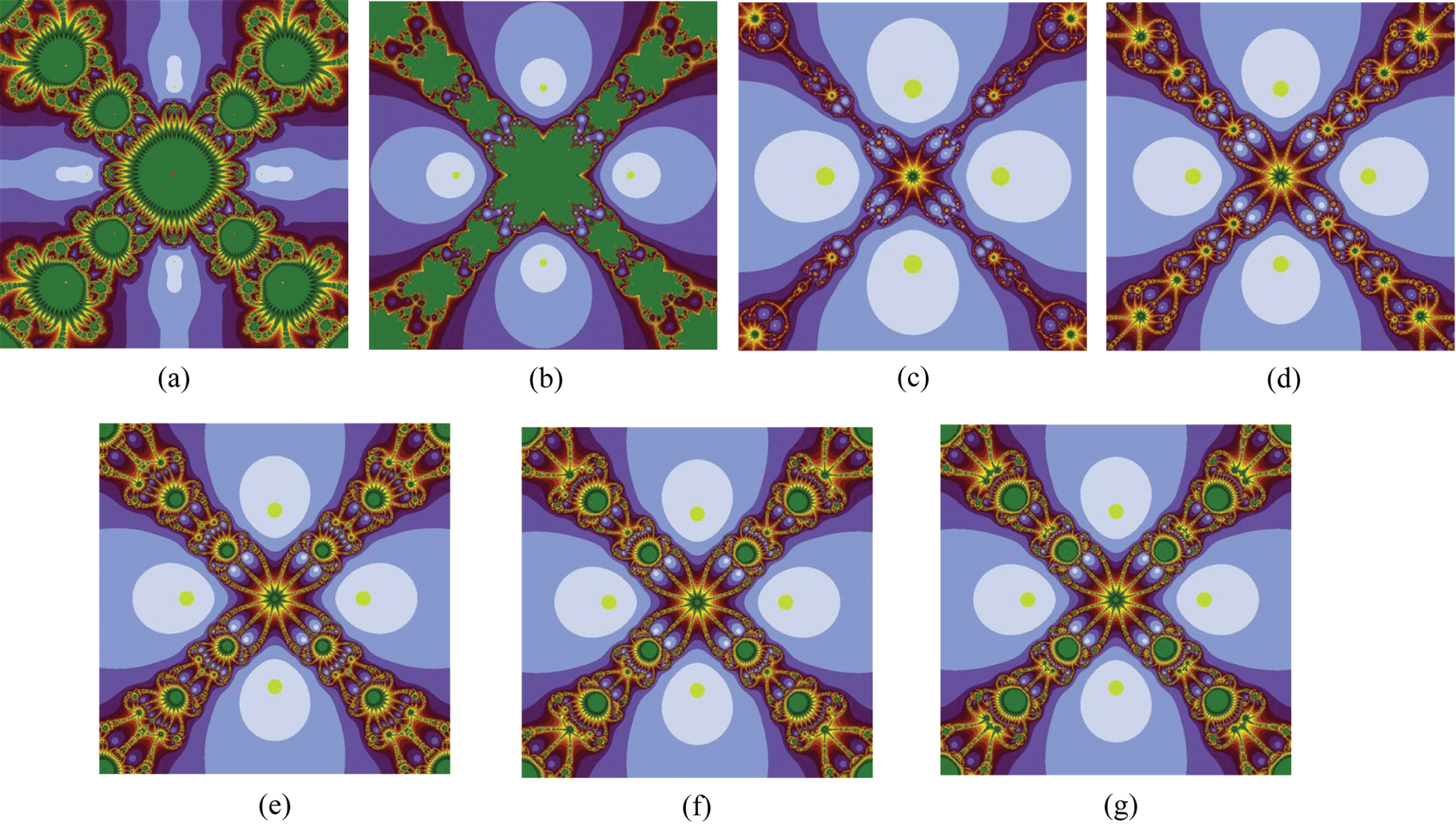
Figure 4: Polynomiographs associated with the polynomial q3(w) . (a) stands for Noor’s method one, (b) stands for Noor’s method two (c) stands for Ostrowski’s method, (d) stands for Traub’s method, (e), (f) and (g) stand for Algorithms 1–3 respectively

5.4 Polynomiographs for the Polynomial q4(w) Using Various Iterative Methods

In the fourth and last experiment, we assume the complex polynomial q4(w)=(w4−1)2, that has four distinct zeros 1,−1,i,and−i out of eight with the multiplicity two. For drawing the polynomiographs of the considered polynomial, we ran all the algorithms via a computer program and the corresponding results in the form of aesthetically pleasing images are given in the following Fig. 5.

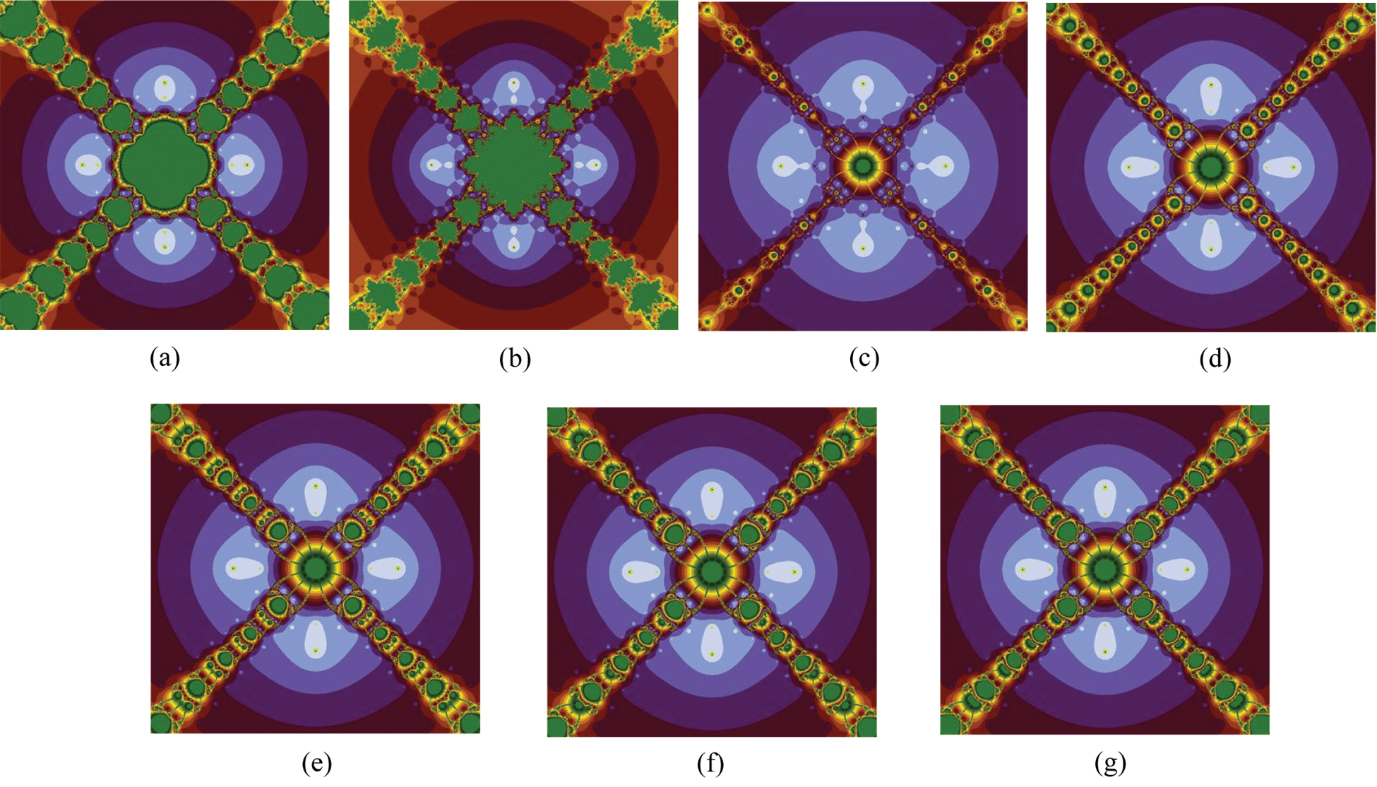
Figure 5: Polynomiographs associated with the polynomial q4(w) . (a) stands for Noor’s method one, (b) stands for Noor’s method two (c) stands for Ostrowski’s method, (d) stands for Traub’s method, (e), (f) and (g) stand for Algorithms 1–3 respectively

In the above experiments, we gave a detailed graphical analysis of the suggested iteration schemes with the other similar-nature two-step iteration schemes using polynomiographs for the different degrees’ complex polynomials with the aid of computer technology. When we look at the generated images, we can read two important characteristics. The first one is the speed of convergence of the iteration scheme, i.e., the color of each point gives us information on how many iterations were performed by the iteration scheme to approximate the root. The second characteristic is the dynamics of the iteration scheme. Low dynamics are in areas where the variation of colors is small, whereas in areas with a large variation of colors the dynamics are high. The black color in images shows that places where the solution cannot be achieved for the given number of iterations. The appearance of the darker region in the above-presented images shows that the considered iteration scheme requires a smaller number of iterations. The areas of the same colors in the above figures indicate the same number of iterations required to determine the solution and they look alike to the contour lines on the map. It can be noted that the polynomiographs generated through our developed iteration schemes contained much brighter and darker areas and did not contain black area as compared to other two-step iteration schemes of the same kind which showing the superiority of the proposed iteration schemes over the other ones. Also, the polynomiographs of the suggested iteration schemes showing a larger convergence area than the other comparable methods which proves the better efficiency of the suggested algorithms.

All these figures have been generated using the computer program Mathematica 12.0 by taking Ԑ=0.001 and M=20 where Ԑ stands for the accuracy and M stands for the upper limit of the number of iterations.

6  Conclusion

Based on exponential series expansion, some novel iteration schemes have been constructed for computing the approximate roots of the non-linear equations with the single variable that possess the quartic convergence order. By solving some arbitrary test problems along with some real-world problems, the applicability, validity, accuracy and performance of the suggested iteration schemes have been analyzed. The numerical results of the Tabs. 1–8 showing better performance and efficiency among the other comparable iteration schemes. We also presented a detailed and comprehensive graphical comparison of the suggested iteration schemes with the other similar-nature two-step iteration schemes in the literature by means of polynomiographs of different complex polynomials that showing the convergence properties and other dynamical features of the suggested iteration schemes. The technique of exponential series expansion can also be applied to construct a new class of root-finding algorithms for the system of non-linear equations.

Funding Statement: The author(s) received no specific funding for this study.

Conflicts of Interest: The authors declare that they have no conflicts of interest to report regarding the present study.

References

 1.  C. Chun, “Construction of Newton-like iteration methods for solving nonlinear equations,” Numeriche Mathematik, vol. 104, pp. 297–315, 2006. [Google Scholar]

 2.  R. L. Burden and J. D. Faires, Numerical Analysis, 6th ed. California, USA: Brooks/Cole Publishing Company, 1997. [Google Scholar]

 3.  J. Stoer and R. Bulirsch, Introduction to Numerical Analysis, 3rd ed. New York, USA: Springer-Verlag, 2002. [Google Scholar]

 4.  A. Quarteroni, R. Sacco and F. Saleri, Numerical Mathematics. New York, USA: Springer-Verlag, 2000. [Google Scholar]

 5.  I. K. Argyros, “A note on the Halley method in Banach spaces,” Applied Mathematics and Computation, vol. 58, pp. 215–224, 1993. [Google Scholar]

 6.  J. M. Gutierrez and M. A. Hernandez, “An acceleration of Newtons method: Super-Halley method,” Applied Mathematics and Computation, vol. 117, pp. 223–239, 2001. [Google Scholar]

 7.  J. M. Gutierrez and M. A. Hernandez, “A family of Chebyshev-Halley type methods in Banach spaces,” Bulletin of the Australian Mathematical Society, vol. 55, pp. 113–130, 1997. [Google Scholar]

 8.  S. Householder, The Numerical Treatment of a Single Nonlinear Equation. New York, USA: McGraw-Hill, 1970. [Google Scholar]

 9.  A. Amiri, A. Cordero, M. T. Darvishi and J. R. Torregrosa, “A fast algorithm to solve systems of nonlinear equations,” Journal of Computational and Applied Mathematics, vol. 354, pp. 242–258, 2019. [Google Scholar]

10. M. A. Noor, K. I. Noor and K. Aftab, “Some new iterative methods for solving nonlinear equations,” World Applied Sciences Journal, vol. 20, no. 6, pp. 870–874, 2012. [Google Scholar]

11. A. M. Ostrowski, Solution of Equations and Systems of Equations, 2nd ed. New york: Academic Press, 1966. [Google Scholar]

12. J. F. Traub, Iterative Methods for the Solution of Equations. New York, USA: Chelsea Publishing company, 1982. [Google Scholar]

13. A. Naseem, M. A. Rehman and T. Abdeljawad, “Numerical algorithms for finding zeros of nonlinear equations and their dynamical aspects,” Journal of Mathematics, vol. 2020, pp. 11, 2020. [Google Scholar]

14. S. A. Sariman and I. Hashim, “New optimal Newton-Householder methods for solving nonlinear equations and their dynamics, CMC-Computers,” Materials & Continua, vol. 65, no. 1, pp. 69–85, 2020. [Google Scholar]

15. A. Naseem, M. A. Rehman and T. Abdeljawad, “Higher-order root-finding algorithms and their basins of attraction,” Journal of Mathematics, vol. 2020, pp. 11, 2020. [Google Scholar]

16. R. Imin and A. Iminjan, “A new SPH iterative method for solving nonlinear equations,” International Journal of Computational Methods, vol. 15, no. 3, pp. 1–9, 2018. [Google Scholar]

17. M. A. Noor, W. A. Khan and A. Hussain, “A new modified Halley method without second derivatives for nonlinear equation,” Applied Mathematics and Computation, vol. 189, pp. 1268–1273, 2007. [Google Scholar]

18. M. S. Rhee, Y. I. Kim and B. Neta, “An optimal eighth-order class of three-step weighted Newton's methods and their dynamics behind the purely imaginary extraneous fixed points,” International Journal of Computer Mathematics, vol. 95, pp. 2174–2211, 2017. [Google Scholar]

19. M. A. Hafiz and S. M. H. Al-Goria, “New ninth and seventh order methods for solving nonlinear equations,” European Scientific Journal, vol. 8, no. 27, pp. 83–95, 2012. [Google Scholar]

20. M. Salimi, N. M. A. NikLong, S. Sharifi and B. A. Pansera, “A multi-point iterative method for solving nonlinear equations with optimal order of convergence,” Japan Journal of Industrial and Applied Mathematics, vol. 35, pp. 497–509, 2018. [Google Scholar]

21. O. S. Solaiman and I. Hashim, “Efficacy of optimal methods for nonlinear equations with chemical engineering applications,” Mathematical Problems in Engineering, vol. 2019, pp. 11, 2019. [Google Scholar]

22. Y. Chu, N. Rafiq, M. Shams, S. Akram, N. A. Mir et al., “Computer methodologies for the comparison of some efficient derivative free simultaneous iterative methods for finding roots of non-linear equations,” Computers Materials & Continua, vol. 66, no. 1, pp. 275–290, 2021. [Google Scholar]

23. I. Mahariq and A. Erciyas, “A spectral element method for the solution of magnetostatic fields,” Turkish Journal of Electrical Engineering and Computer Sciences, vol. 25, pp. 2922–2932, 2017. [Google Scholar]

24. H. Ahmad, A. R. Seadawy and T. A. Khan, “Numerical solution of Korteweg-de Vries-Burgers equation by the modified variational iteration algorithm-II arising in shallow water waves,” Physica Scripta, vol. 95, pp. 045210, 2020. [Google Scholar]

25. I. Mahariq, “On the application of the spectral element method in electromagnetic problems involving domain decomposition,” Turkish Journal of Electrical Engineering and Computer Sciences, vol. 25, pp. 1059–1069, 2017. [Google Scholar]

26. I. Mahariq and H. Kurt, “Strong field enhancement of resonance modes in dielectric microcylinders,” Journal of the Optical Society of America B, vol. 33, pp. 656–662, 2016. [Google Scholar]

27. M. A. Rehman, A. Naseem and T. Abdeljawad, “Some novel sixth-order iteration schemes for computing zeros of nonlinear scalar equations and their applications in engineering,” Journal of Function Spaces, vol. 2021, pp. 11, 2021. [Google Scholar]

28. I. Mahariq, H. I. Tarman and M. Kuzuoglu, “On the accuracy of spectral element method in electromagnetic scattering problems,” International Journal of Computer Theory and Engineering, vol. 6, pp. 495–499, 2014. [Google Scholar]

29. Q. M. Al-Mdallal, H. Yusuf and A. Ali, “A novel algorithm for time-fractional foam drainage equation,” Alexandria Engineering Journal, vol. 59, pp. 1607–1612, 2020. [Google Scholar]

30. H. Ahmad, A. R. Seadawy, A. H. Ganie, S. Rashid, T. A. Khan et al., “Approximate numerical solutions for the nonlinear dispersive shallow water waves as the Fornberg-Whitham model equations,” Results in Physics, vol. 22, pp. 103907, 2021. [Google Scholar]

31. Q. M. Al-Mdallal, M. Al-Refai, M. Syam and K. M., “Al-Srihin theoretical and computational perspectives on the eigenvalues of fourth-order fractional Sturm-Liouville problem,” International Journal of Computer Mathematics, vol. 95, pp. 1548–1564, 2018. [Google Scholar]

32. J. Jin, L. Zhao, M. Li, F. Yu and Z. Xi, “Improved zeroing neural networks for finite time solving nonlinear equations,” Neural Computing and Applications, vol. 32, pp. 4151–4160, 2020. [Google Scholar]

33. Q. M. Al-Mdallal and A. S. A. Omer, “Fractional-order Legendre-collocation method for solving fractional initial value problems,” Applied Mathematics and Computation, vol. 321, pp. 74–84, 2018. [Google Scholar]

34. H. Ahmad, A. Akgul, T. A. Khan, P. S. Stanimirovic and Y. M. Chu, “New perspective on the conventional solutions of the nonlinear time-fractional partial differential equations,” Complexity, vol. 2020, pp. 10, 2020. [Google Scholar]

35. V. D. Waals and J. Diderik, “Over de Continuiteit van den Gas-en Vloeistoftoestand (on the continuity of the gas and liquid state),” Ph.D. thesis, Leiden, The Netherlands, 1873. [Google Scholar]

36. M. Planck, The Theory of Heat Radiation, Translated by Masius, M. 2nd ed., OL 7154661M. P. Blakiston’s Son & Co, 1914. [Google Scholar]

37. M. S. E. Kehat, “An iteration method with memory for the solution of a non-linear equation,” Chemical Engineering Science, vol. 27, pp. 2099–2101, 1972. [Google Scholar]

38. S. Weerakoon and T. G. I. Fernando, “A variant of Newton’s method with accelerated third-order convergence,” Applied Mathematics Letters, vol. 13, pp. 87–93, 2000. [Google Scholar]

39. B. Kalantari, “Polynomiography from the fundamental theorem of Algebra to art,” Leonardo, vol. 38, no. 3, pp. 233–238, 2005. [Google Scholar]

40. B. Kalantari, “Method of creating graphical works based on polynomials.” U.S. Patent 6, 894, 705, 2005. [Google Scholar]

41. B. Mandelbrot, The Fractal Geometry of Nature. New York, USA: W.H. Freeman and Company, 1983. [Google Scholar]

42. B. Kalantari and E. H. Lee, “Newton-Ellipsoid polynomiography,” Journal of Mathematics and the Arts, vol. 13, no. 4, pp. 336–352, 2019. [Google Scholar]

43. K. Gdawiec, “Fractal patterns from the dynamics of combined polynomial root finding methods,” Nonlinear Dynamics, vol. 90, no. 4, pp. 2457–2479, 2017. [Google Scholar]

44. S. M. Kang, A. Naseem, W. Nazeer, M. Munir and C. Yong, “Polynomiography via modified Abbasbanday's method,” International Journal of Mathematical Analysis, vol. 11, no. 3, pp. 133–149, 2017. [Google Scholar]

45. K. Gdawiec, W. Kotarski and A. Lisowska, “Visual analysis of the Newton’s method with fractional order derivatives,” Symmetry, vol. 11, no. 9, pp. 27, 2019. [Google Scholar]

46. J. R. Sharma and H. Arora, “A new family of optimal eighth order methods with dynamics for non-linear equations,” Applied Mathematics and Computation, vol. 273, pp. 924–933, 2016. [Google Scholar]

47. A. Naseem, M. A. Rehman and T. Abdeljawad, “Numerical algorithms for finding zeros of nonlinear equations and their dynamical aspects,” Journal of Mathematics, vol. 2020, pp. 11, 2020. [Google Scholar]

48. B. Neta, M. Scott and C. Chun, “Basins of attraction for several methods to find simple roots of nonlinear equations,” Applied Mathematics and Computation, vol. 218, pp. 10548–10556, 2012. [Google Scholar]

This work is licensed under a Creative Commons Attribution 4.0 International License, which permits unrestricted use, distribution, and reproduction in any medium, provided the original work is properly cited.