DOI:10.32604/iasc.2021.018643
| Intelligent Automation & Soft Computing DOI:10.32604/iasc.2021.018643 | |
| Article |
Visual Saliency Prediction Using Attention-based Cross-modal Integration Network in RGB-D Images
1School of Computer Science and Cyberspace Security, Hainan University, 570228, Haikou, China
2School of Information and Electronic Engineering, Zhejiang University of Science & Technology, 310023, Zhejiang, China
3Department of Computer Science and Engineering, Michigan State University, 48913, Michigan, USA
*Corresponding Author: Ting Jin. Email: tingj@fudan.edu.cn
Received: 14 March 2021; Accepted: 15 April 2021
Abstract: Saliency prediction has recently gained a large number of attention for the sake of the rapid development of deep neural networks in computer vision tasks. However, there are still dilemmas that need to be addressed. In this paper, we design a visual saliency prediction model using attention-based cross-model integration strategies in RGB-D images. Unlike other symmetric feature extraction networks, we exploit asymmetric networks to effectively extract depth features as the complementary information of RGB information. Then we propose attention modules to integrate cross-modal feature information and emphasize the feature representation of salient regions, meanwhile neglect the surrounding unimportant pixels, so as to reduce the lost of channel details during the feature extraction. Moreover, we contribute successive dilated convolution modules to reduce training parameters and to attain multi-scale reception fields by using dilated convolution layers, also, the successive dilated convolution modules can promote the interaction of two complementary information. Finally, we build the decoder process to explore the continuity and attributes of different levels of enhanced features by gradually concatenating outputs of proposed modules and obtaining final high-quality saliency prediction maps. Experimental results on two widely-agreed datasets demonstrate that our model outperforms than other six state-of-the-art saliency models according to four measure metrics.
Keywords: Saliency prediction; attention modules; dilated convolution; RGB-D
Nowadays, with the wake and development of computer vision, visual saliency prediction becomes a fundamental and challenging task. Visual saliency prediction in computer vision aims at predicting the eye fixation of humankind and mimicking this ability to process the flood of visual information so as to highlight salient regions and neglect the background in a short time. The research of saliency prediction models leads the development to many applications, such as quality assessment [1–3], image segmentation [4,5], object detection [6–10], and object tracking [11–16]. However, there are still two challenges that need to be addressed. First, excavate strong strategies to extract multi-level and multi-scale information and use rich semantic information to predict human eye-fixation. Second, remedy the lost of details during feature extraction and effectively suppress the redundant and unimportant information to select the most prominent or salient objects from different and even complex situations.
To break out of aforementioned challenges, we build a network with asymmetric feature extraction strategy based on attention mechanism and successive dilated convolution layers. As shown in Fig. 1, the network first extracts multi-scale and multi-level RGB and depth features. Since attention models can excavate rich and significant contextual information by assigning different weighted value to corresponding regions according to the importance and prominence of each region in images, we then integrate RGB and depth features on the same level, and input them into an attention module. Next we deliver the highest level features of RGB and depth streams into two successive dilated convolution modules. Finally, we aggregate the results of attention modules with the output feature maps of dilated convolution modules, and gradually upsample them in the decoder process. Experiments show that our model outperforms than other six state-of-the-art saliency models.
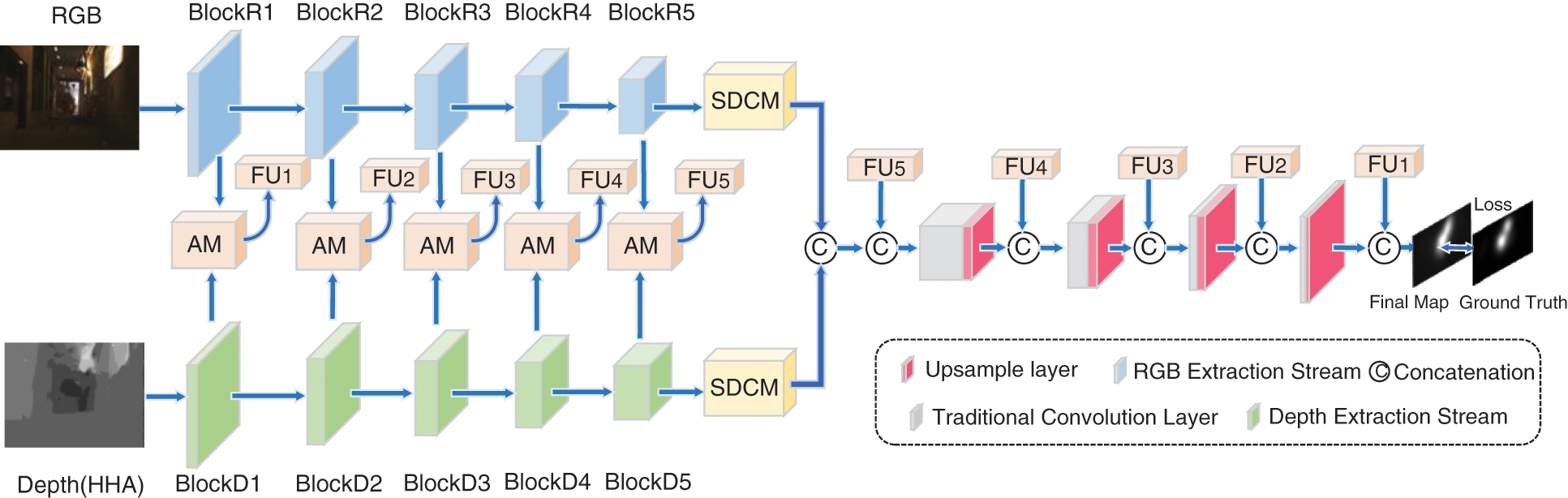
Figure 1: The overall architecture of the proposed saliency prediction model. We leverage asymmetric encoders to extract RGB and depth features. The output of each encoder is sent into following SDCM and concatenated with the output of AM (FUi, i = 1, 2 … 5) gradually in the decoder process
The main contributions of this work are summarized as follows: 1) we adopt an asymmetric extraction network to obtain multi-scale and multi-model feature information, 2) we propose attention modules to deal with the lose of feature details, emphasize salient regions in RGB-D images with cross-modal integration, 3) we design successive dilated convolution modules to enhance the capability of excavating interior perception of visual features and emphasizing the feature representation.
The remainder of this paper is organized as follows. Section 2 provides a brief survey of related work. We detail the proposed network in Section 3. Experimental results on saliency prediction are reported in Section 4. Finally, we draw conclusions in Section 5.
Conventional saliency prediction models are most biologically inspired, some of them mainly defined and captured biological evidences, such as color, texture, contrast, others exploit higher semantic concepts, such as faces, cars, and people. For instance, Xu et al. [17] proposed a global-contrast-based saliency model using the weighted mean vector and including color, chromatic double opponency, and similarity distribution, to increase the detection precision and neglect the surrounding pixels of salient regions. Take the advantages of the Gestalt principles, Zou et al. [18] proposed a surroundedness-based multiscale saliency method, which integrates the background priors, multiscale saliency maps and the final saliency maps, to conduct figure-ground segregation. Recently, with the large spread of deep neural convolution (DNN), the saliency prediction studies have achieved unprecedented improvement. For example, Kroner et al. [19] predicted the human eye-fixation by designing a network with encoder-decoder structure to extract multi-scale features by different parallel dilated convolution layers. Wang et al. [20] proposed the attentive saliency network to detect salient objects from fixation maps. Dodge et al. [21] built a network called MxSalNet to contain global scene semantic information in addition to local information gathered by a convolutional neural network (CNN), so as to predict saliency for a set of closely related images. Bak et al. [22] proposed a spatio-temporal saliency network with two-stream fusion mechanism to predicts saliency maps. Liu et al. [23] proposed a saliency model that considers saliency as descriptions of the combination of simple features and captures multiple contexts, finally produces saliency maps in a comprehensive way.
Despite saliency models in 2D images have reached comparable improvement, most of them are absent of geological cues as auxiliary information for better predicting saliency attributes. With the advent of RGB-D sensors, depth information plays an important role in assisting RGB information as a supplement to locate human eye-fixation points. For example, Huang et al. [24] proposed an end-to-end DNN with the fusion strategy in higher layers for RGB-D saliency prediction. Li et al. [25] proposed a saliency model in 3D images using the Siamese structures, which is fused in an interactive and adaptive way. Yang et al. [26] designed a two-stage clustering scheme to deal with the negative influence of impaired depth videos so as to predict human visual fixation in dynamic scenarios. Nowadays, many researches are inspired by visual attention mechanism of human beings, and introduce attention models to DNN, which is a great improvement for the accuracy and availability of saliency algorithms. For example, Zhou et al. [27] proposed an RGB-D saliency model by applying the combination of the attention-guided bottom-up and top-down modules, and the multi-level RGB and related depth features. Zhu et al. [28] presented a saliency DNN model aggregating the attentional dilated features. Zhou et al. [29] proposed a flow-driven attention network called FDAN to make full use of motion information for video saliency.
In this section, we will first briefly discuss the proposed saliency prediction model in Sec. 3.1. And we will describe the asymmetric feature extractor in Sec. 3.2. Then, we will give a detailed demonstration of attention modules in Sec. 3.3. Next, we will elaborate successive dilated convolution modules in Sec. 3.4. Finally, we will describe the decoder in Sec. 3.5.
As shown in Fig. 1, the proposed saliency model is based on four major components: the asymmetric feature extractor (named as AFE), the cross-model integration attention modules (named as AM), the successive dilated convolution modules (named as SDCM) and the decoder. AFE has two asymmetric encoders, of which one stream extracts the RGB information and the other stream learns corresponding depth vectors. AMs fuse RGB and paired depth features and enhance the feature representation. Two SDCMs have the same structures. The only difference between two SDCMs is that they follow the end of the RGB stream and depth stream, respectively. The decoder connects the output saliency maps of AM and SDCM and further excavates the progression of different levels of enhanced features.
3.2 Asymmetric Feature Extractor (AFE)
Considering the depth maps are single-channel, which cannot reflect abundant geometrical cues, we transform the depth maps into three-channel HHA [30] images. Although the Siamese encoder structure effectively reduces the trainable parameters and increases the accuracy of saliency models, it also brings several bottlenecks in saliency prediction. Therefore, we design the AFE in order to fully extract multiscale and cross-modal features in five layers, as well as reduce the Gradient descent. The AFE contains the RGB extraction stream and the depth extraction stream. For a fair comparison with other state-of-the-art saliency models, we use modified ResNet-50 [31] as the backbone network for the RGB extraction stream. Concretely, we remove its average pooling layers and fully connected layers. Similarly, we remain the five convolutional blocks of VGG-16 [32], removing the average pooling layers and fully connected layers, as the backbone network for the depth extraction stream. Then, we pretrained both RGB and depth extraction branches and initiate the parameters on the ImageNet database [33].
We represent features of five-stage RGB stream (BlockRi in Fig. 1) as
3.3 Cross-modal Integration Attention Module (AM)
Since salient regions or objects exist in not only RGB images but also depth images, we sufficiently integrate cross-modal complementarity between corresponding RGB and depth images. Besides, during the feature extraction of both the RGB stream and paired depth stream, channel details of hierarchical features
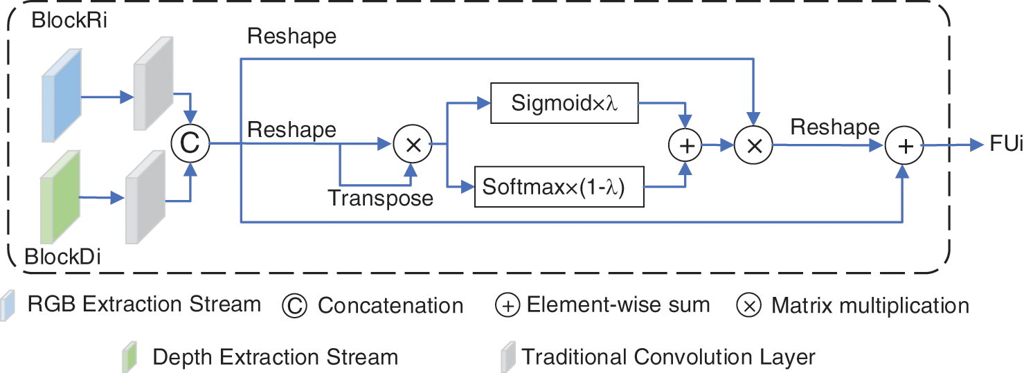
Figure 2: The cross-model integration attention module
We first feed
where T represents the transpose operation, and
where
We conduct the matrix multiplication between A and
where α is a learnable parameter initialized to zero.
3.4 Successive Dilated Convolution Module (SDCM)
The asymmetric network extracts multi-scale features, and features in high levels include rich and informative semantic information. For the purpose of making full use of those semantic information and remedying shortages of the feature extraction in ordinary convolution layers, we propose the successive dilated convolution module. The successive dilated convolution module consists of three parallel dilation branches with skip connections, and the structure is depicted in Fig. 3. The final feature maps of SDCM are obtained from a maxpooling layer. Each main branch of SDCM adopts a convolution layer followed by a dilated convolution layer. Then a skip branch, containing a convolution layer and a dilated convolution layer, concatenates with the main branch. Finally, the result becomes the input of next main branch. In this manner, we build the SDCM.
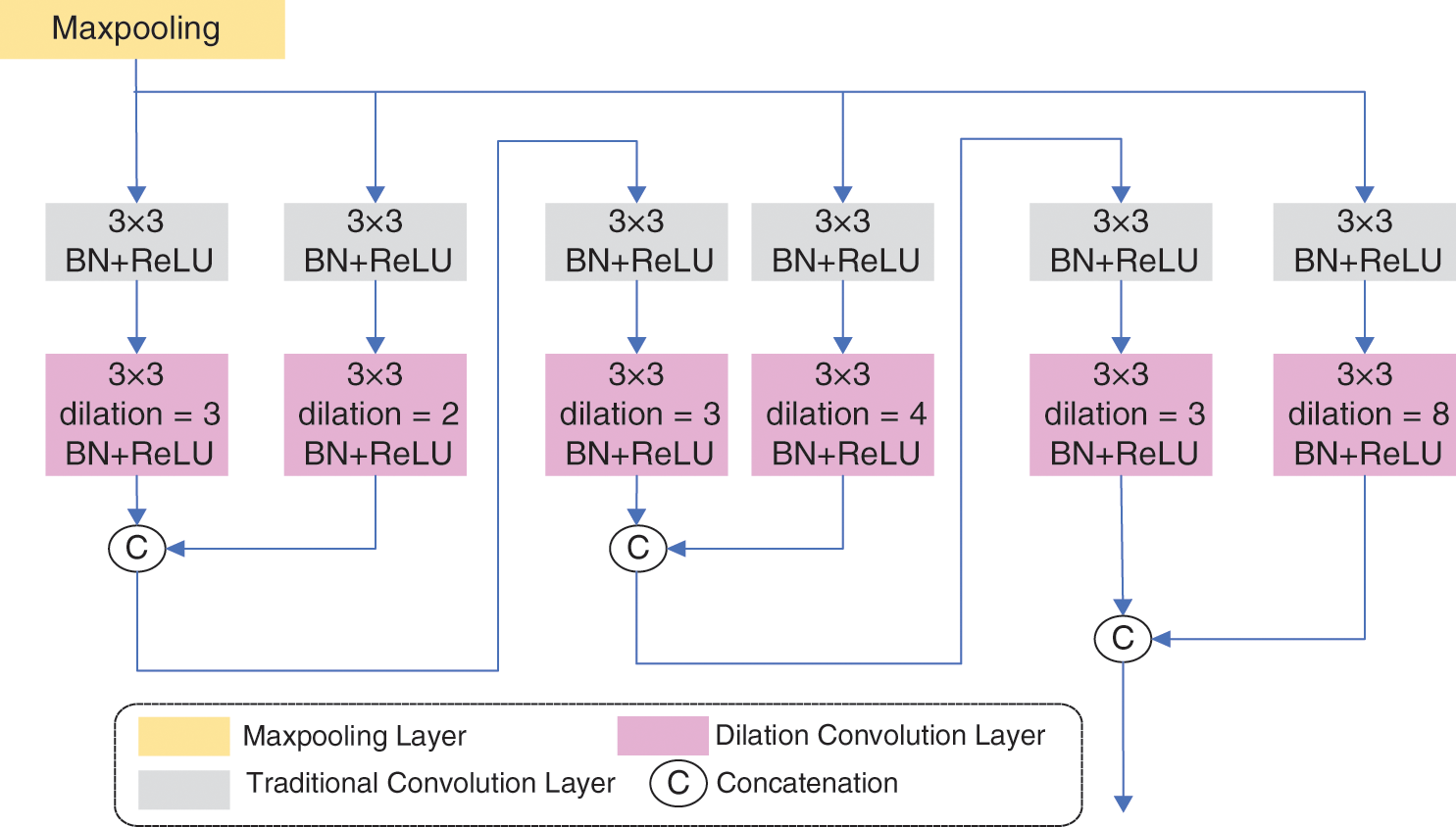
Figure 3: The overall structure of the successive dilated convolution module. 3 × 3 represents the size of convolution kernels. The dilation means the dilation rate in dilated convolution, and the BN +ReLU means the Batchnormal layer and the rectified linear unit (ReLU) activation
Specifically, the first main branch contains the first traditional convolution layer with 3 × 3 kernels, and the first dilated convolution layer, in which the dilation rate is set to 3. Then in the subsequent main branches, the kernels of convolution layers remain the same as the first convolution layer’s, and so are the dilation rate of subsequent dilation rates of dilated convolution layers. All the convolution layers are followed by a BN layer and a ReLU activation:
where conv denotes traditional convolution operation and dil denotes dilated convolution operation. σ represents the Batchnormalization operation and γ represents the ReLU activation. Here we omit the weights and biases. The first skip branch includes a traditional convolution layer with 3 × 3 kernels and the dilation rate of a following dilated convolution layer is set to 2, then the kernels of convolution layers keep the same as the first skip branch’s, and the dilation rates double in the subsequent skip branches. Finally, the main branch concatenates with the skip branch:
where concat means the concatenate operation.
Considering that AM has the capability to enhance all the five-level cross-modal features, and integration features FUi output by AM contain multi-scale information from high-level semantic information to low-level CNN features, we construct a decoder using the FUi to assist the refinement process. As shown in Fig. 1, the combination of two RMs is the input of the decoder. We use the bilinear interpolation to upsample feature maps to restore resolution:
where
For the loss function, we combine the mean squared error with the Kullback–Leibler divergence (KLDiv) to supervise the training of proposed network. KLDiv determines the difference between the predicted and real distributions, which helps to measure the amount of information lost using one distribution to approximate the other. However, KLDiv is always non-negative, and thus we apply the cross-entropy as auxiliary function, which is approaching zero as the error reduces. Given D-dimensional images, the loss function is defined as follows:
where
To prove the capability of our proposed network, we conduct a series of experiments. In the following subsections, we first introduce details of the datasets and the implementation protocol. Subsequently, ablation studies of each component in our approach were conducted. Finally, we compared four evaluation measures on the two datasets with six state-of-the-art methods of real-time semantic segmentation.
In order to evaluate the proposed network, we conducted the experiments on two public representative saliency datasets. These two datasets contain images with rich various scene information and intricate backgrounds, which mainly captured from real-world scenes and 3D movie scenes.
NUS Saliency dataset [37] is a dataset containing 575 pairs of RGB and depth image, which are viewed by 80 participants and provide the color stimuli, corresponding depth maps, and the ground truth represented in the form of fixation maps. It is separated into a training set (420 images), a validation set (60 images) and a testing set (95 images).
NCTU Fixation dataset [38] consists of 500 2D images and their depth images with a resolution of 1920 × 1080. This dataset is mainly from various scenes in existing 3D movies or video, and it includes left view maps, right view maps, depth maps, and monocular and binocular visual fixation maps. This dataset contains divided into a training set (332 images), a validation set (48 images), and a testing set (120 images).
We conducted our implementation protocol on a workstation with a GeForce GTX TITAN XP GPU cards with 12 GB RAM and we used software code written in the publicly available PyTorch 1.1.0 framework [39]. For the backbones, we pretrained the VGG-16 and ResNet-50 networks on the ImageNet database. Then, we fine-tuned the pretrained networks to achieve the high accuracy. We used ReLU activation for the entire architecture. For data augmentation, we exploited horizontal flipping, cropping, and panning to each image and random-sorting channels. We cropped the input RGB-D images to the size of 256 × 256 pixels. In order to avoid the insufficient memory caused by a large amount of data, we appropriately reduce the batch size of each iteration to one and set the initial learning rate to 5E−4. The parameters of the proposed architecture were learned by the backpropagation over 70 epochs.
We adopted four widely-agreed metrics to measure our saliency model to measure the performance of the proposed model: Linear correlation coefficient (CC), Kullback-Leibler Divergence (KL-Div), area under the curve (AUC), and normalized scanpath saliency (NSS).
1) CC is a statistic used to reflect the degree of linear correlation between the final saliency maps proposed model (S) and the ground truth (G). The closer the CC value is to 1 or −1, the better the saliency prediction algorithm is. We use cov to denote the covariance between the S and G, and CC is formulated as:
2) KLDiv, also known as relative entropy or information divergence, is an asymmetric measure of the difference between two probability distributions. The smaller the KLDiv value is, the better the performance of the network is. Given two probability distributions for x, which are denoted as a(x) and b(x). KLDiv is defined as:
3) AUC is defined as the area under the ROC curve. The reason why AUC value is used as the evaluation standard of the model is that in many cases, the ROC curve cannot clearly indicate which classifier has better performance. AUC is a kind of evaluation index to measure the quality of dichotomy model, which indicates the probability that the predicted positive cases rank before the negative ones. As a numerical value, the model with larger AUC has better performance. AUC can be represented as:
where pos represents positive instances, and k is the ranking. ∑posk is a permanent value, which is only relevant with the total number of positive instances. Npos and Nneg denote the number of positive and negative instances, respectively.
4) NSS is defined by the average value of human eye-fixation points in saliency prediction model. The bigger the NSS value is, the better the performance of the saliency prediction model is.
4.4 Ablation Study and Analyses
To verify the performance of proposed AFE, AM and SDCM, we implement ablation experiments with different settings. We mainly report the results conducting on the NCTU dataset.
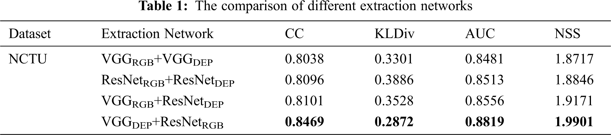
1) Availability of AFE: AFE is used to fully extract multi-scale and multi-modal information. To confirm the effectiveness of AFE, we remained other components of the proposed network, but changed the feature extraction network, namely, VGGRGB+VGGDEP, ResNetRGB+ResNetDEP, VGGRGB+ResNetDEP and VGGDEP+ResNetRGB. The subscript of RGB and DEP represent the backbone network of RGB and depth extraction stream, respectively. For instance, VGGRGB means the backbone of RGB extraction network is VGG-16. Tab. 1 shows that the combination of asymmetric networks can bring a better performance. Furthermore, using VGG-16 extracting depth information and ResNet-50 extracting RGB information can obtain the best result.
2) Availability of AM: AM is used to strengthen the feature representation and reduce the lost of details. To testify the availability of AM, we remove the AM from the proposed network, which is denoted as P-A. Tab. 2 shows that the AM is beneficial to the performance of the proposed saliency model. Besides, Fig. 4 visually reflects that final saliency maps in the fourth column are quite indistinct. Thus, the AM can improve the quality of final saliency maps.
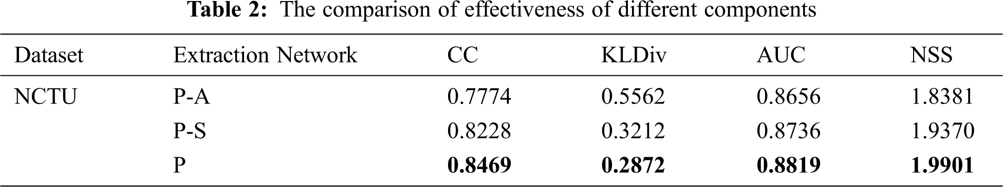
3) Availability of SDCM: SDCM can effectively integrate the feature information of different scales for the sake of boosting the feature invariance. To prove the validity of SDCM, we remove the SDCM from the proposed network, which is denoted as P-S. Tab. 2 demonstrates that the SDCM increases the results of four evaluation metrics. Meanwhile, the fifth column in Fig. 4 exhibits that the involvement of SDCM enhances the detail representation of final saliency maps.
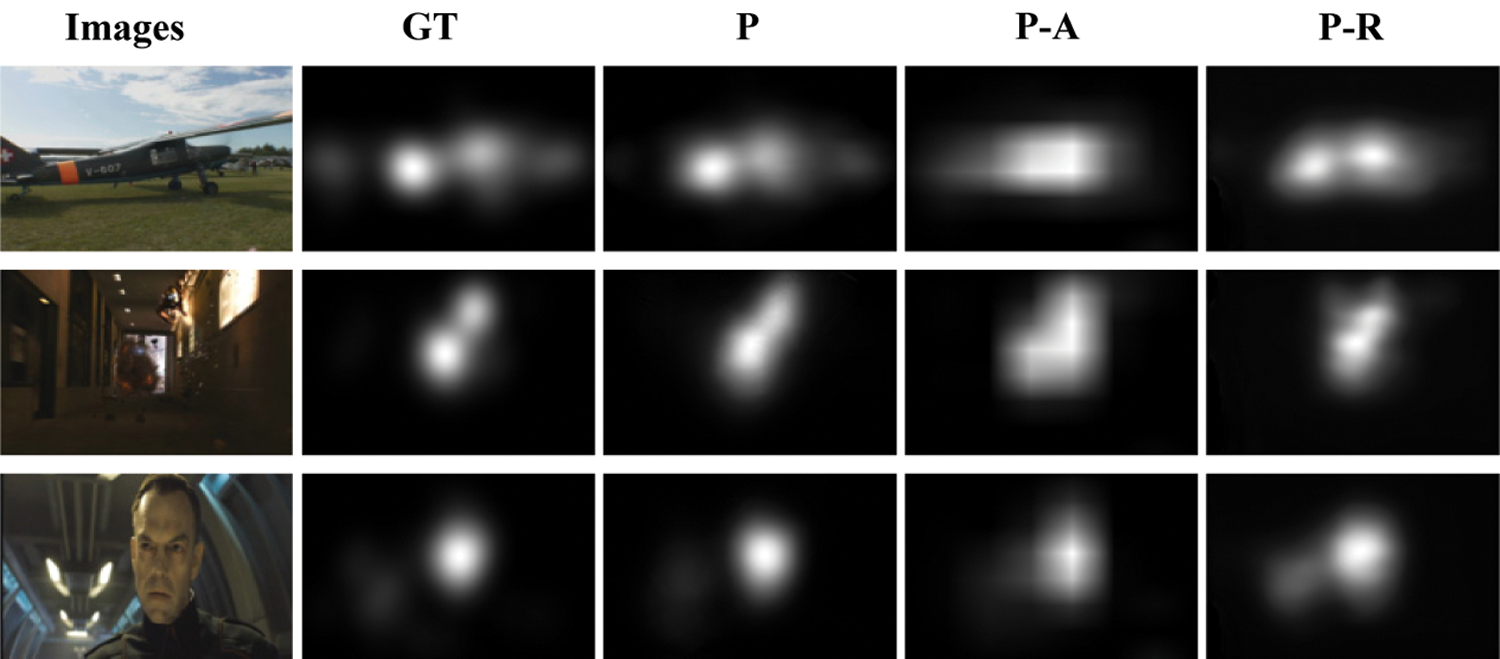
Figure 4: Visual comparisons of different components
4.5 Comparison with Six State-of-the-art
We contrasted the proposed method with six state-of-the-art saliency prediction models, including two networks with two-stream structures, i.e. Fang et al. [40] and Qi et al. [41], and four saliency models in 2D images, i.e. DeepFix [42], ML-Net [43], DVA [44], and MSI-Net [45]. We rebuilt the four RGB saliency models through adding a depth stream, which is used as the supplement to the RGB stream. All parameter settings are according to the recommendation of their authors. We used the same training sets, validation sets, and test sets to train above saliency models. As shown in Tab. 3, the proposed architecture achieved the biggest CC, AUC and NSS scores, and lowest KLDiv scores on two datasets.
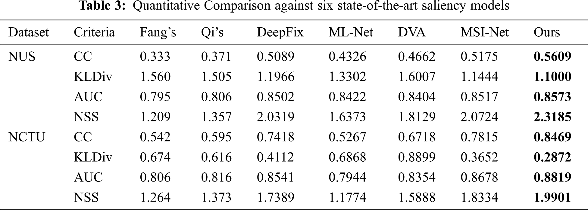
This result shows that the proposed network consistently outperforms six state-of-the-art models on the NCTU and NUS datasets. Some heatmaps simulated the eye-fixation generated by the proposed network and the six state-of-the-art saliency models are shown in Fig. 5 for a subjective comparison. It can be seen that our method has produced a more precise saliency maps in different challenging situations: single objects in simple background (rows 1, 8 in Fig. 5), single objects in complex backgrounds (rows 3, 4, 5, 7 in Fig. 5), multiple objects in simple background (row 2 in Fig. 5), and multiple objects in sophisticated background (row 6 in Fig. 5). Fig. 5 also shows that our model can handle both low contrast (row 5, 6, 7) cases. These results demonstrate the robustness and effectiveness of our model, and verify the availability of the AFE, AM and SDCM.
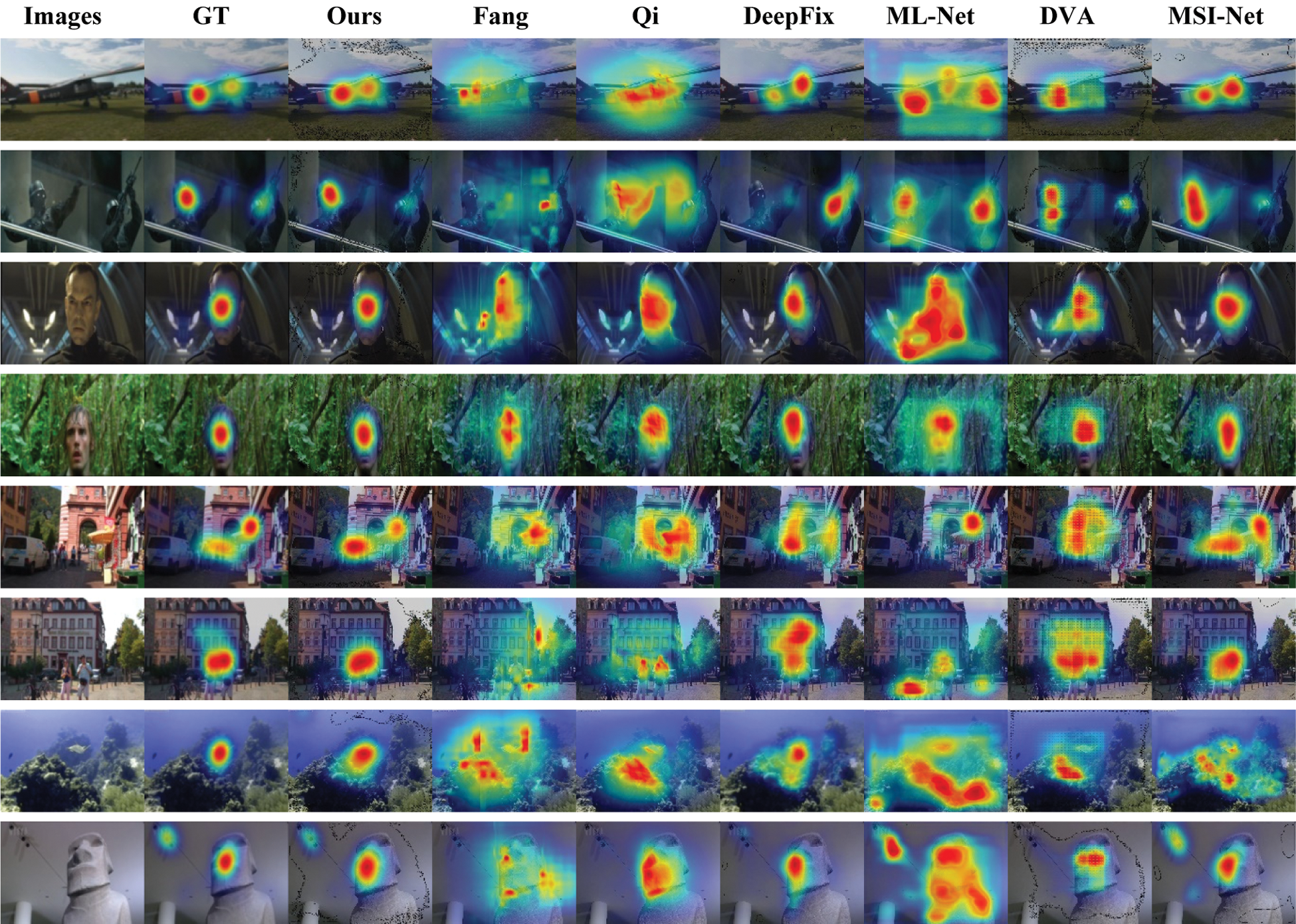
Figure 5: Visual comparisons to six state-of-the-art saliency models on NCTU dataset
Although our model can suppress the background and highlight the prominent salient regions more effectively than other compared methods, there are still shortages. Fig. 6 demonstrates failure cases of the proposed network. Column 1 contains the original RGB images, column 2 includes the ground truth of simulated eye-fixation, column 3 consists of eye-fixation maps obtained by our network, column 4 contains the ground truth of final saliency maps, and the last column includes final saliency maps produced by our architecture. As shown in Fig. 6, our model cannot handle two specific situations effectively: relatively small-scale and large-scale objects in complex background (row 1, 2 in Fig. 6, respectively).
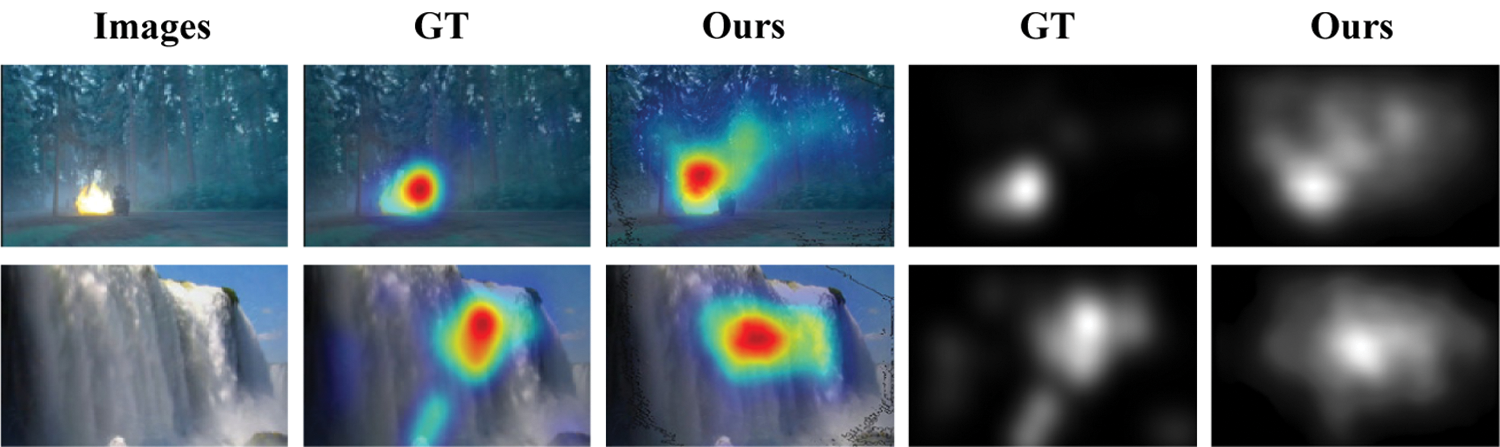
Figure 6: Failure cases of three specific situations
We design a visual saliency prediction network on the basis of attention mechanism and cross-model integration strategies in RGB-D images. We first leverage asymmetric networks to extract two complementary information of RGB information and depth information as cross-model features. To achieve using cross-model information and accurately predict the human eye-fixation in complex situations, we propose attention modules to integrate them, and attention modules can enhance salient regions and lighten the surrounding unimportant background. To further reduce parameters for training and promote the interaction of cross-modal features, we build successive dilated convolution modules. Then we gradually aggregate salient features. Finally, the decoder process provides high-quality final saliency prediction maps. Experimental results on two widely-agreed datasets demonstrate that our model outperforms than other six state-of-the-art saliency models. In future work, we will improve and generalize the proposed method for low contrast scenarios and apply the network in different computer vision applications.
Funding Statement: This paper was supported by the National Nature Science Foundation of China (61862021); the Hainan Provincial Natural Science Foundation of China (620RC565); and the Innovative Research Projects of Graduate Students of Hainan Province (Hys2020-91).
Conflicts of Interest: The authors declare that they have no conflicts of interest to report regarding the present study.
1. I. Abouelaziz, A. Chetouani, M. El Hassouni, L. Jan Latecki and H. Cherifi, “3D visual saliency and convolutional neural network for blind mesh quality assessment,” Neural Comput & Applic, vol. 32, pp. 16589–16603, 2020. [Google Scholar]
2. K. Gu, S. Wang, H. Yang, W. Lin, G. Zhai et al., “Saliency-guided quality assessment of screen content images,” IEEE Transactions on Multimedia, vol. 18, no. 6, pp. 1098–1110, 2016. [Google Scholar]
3. L. Tang, Q. Wu, W. Li and Y. Liu, “Deep saliency quality assessment network with joint metric,” IEEE Access, vol. 6, pp. 913–924, 2018. [Google Scholar]
4. S. Joon Oh, R. Benenson, A. Khoreva, Z. Akata, M. Fritz et al., “Exploiting saliency for object segmentation from image level labels,” in Proc. CVPR, Hawaii, USA, pp. 4410–4419, 2017. [Google Scholar]
5. Y. Zeng, Y. Zhuge, H. Lu and L. Zhang, “Joint learning of saliency detection and weakly supervised semantic segmentation,” in Proc. ICCV, Seoul, Korea, pp. 7223–7233, 2019. [Google Scholar]
6. Q. Hou, M. Cheng, X. Hu, A. Borji, Z. Tu et al., “Deeply supervised salient object detection with short connections,” IEEE Transactions on Pattern Analysis and Machine Intelligence, vol. 41, no. 4, pp. 815–828, 2019. [Google Scholar]
7. Q. Zhang, N. Huang, L. Yao, D. Zhang, C. Shan et al., “RGB-T salient object detection via fusing multi-level cnn features,” IEEE Transactions on Image Processing, vol. 29, pp. 3321–3335, 2020. [Google Scholar]
8. J. Zhao, J. Liu, D. Fan, Y. Cao, J. Yang et al., “EGNet: Edge guidance network for salient object detection,” in Proc. CVPR, Long Beach, CA, USA, pp. 8778–8787, 2019. [Google Scholar]
9. J. Mai, X. Xu, G. Xiao, Z. Deng and J. Chen, “PGCA-Net: Progressively aggregating hierarchical features with the pyramid guided channel attention for saliency detection,” Intelligent Automation & Soft Computing, vol. 26, no. 4, pp. 847–855, 2020. [Google Scholar]
10. L. Feng, H. Li, Y. Gao and Y. Zhang, “The application of sparse reconstruction algorithm for improving background dictionary in visual saliency detection,” Intelligent Automation & Soft Computing, vol. 26, no. 4, pp. 831–839, 2020. [Google Scholar]
11. H. Lee and D. Kim, “Salient region-based online object tracking,” in Proc. WACV, Lake Tahoe, NV/CA, USA, pp. 1170–1177, 2018. [Google Scholar]
12. F. Bi, X. Ma, W. Chen, W. Fang, H. Chen et al., “Review on video object tracking based on deep learning,” Journal of New Media, vol. 1, no. 2, pp. 63–74, 2019. [Google Scholar]
13. B. Hu, H. Zhao, Y. Yang, B. Zhou and A. Noel, “Multiple faces tracking using feature fusion and neural network in video,” Intelligent Automation & Soft Computing, vol. 26, no. 6, pp. 1549–1560, 2020. [Google Scholar]
14. D. Huang, P. Gu, H. Feng, Y. Lin and L. Zheng, “Robust visual tracking models designs through kernelized correlation filters,” Intelligent Automation & Soft Computing, vol. 26, no. 2, pp. 313–322, 2020. [Google Scholar]
15. X. Fan, C. Xiang, C. Chen, P. Yang, L. Gong et al., “BuildSenSys: Reusing building sensing data for traffic prediction with cross-domain learning,” arXiv: eess.SP, arXiv:2003.06309, 2020. [Google Scholar]
16. C. Avytekin, F. Cricri and E. Aksu, “Saliency enhanced robust visual tracking,” in Proc. EUVIP, Tampere, Finland, pp. 1–5, 2018. [Google Scholar]
17. L. Xu, L. Zeng and H. Duan, “An effective vector model for global-contrast-based saliency detection,” Journal of Visual Communication and Image Representation, vol. 30, pp. 64–74, 2015. [Google Scholar]
18. B. Zou, Q. Liu, Z. Chen, H. Fu and C. Zhu, “Surroundedness based multiscale saliency detection,” Journal of Visual Communication and Image Representation, vol. 33, pp. 378–388, 2015. [Google Scholar]
19. A. Kroner, M. Senden, K. Driessens and R. Goebel, “Contextual encoder-decoder network for visual saliency prediction,” Neural Networks, vol. 129, pp. 261–270, 2020. [Google Scholar]
20. W. Wang, J. Shen, X. Dong and A. Borji, “Salient object detection driven by fixation prediction,” in Proc. CVPR, Salt Lake City, UT, USA, pp. 1711–1720, 2018. [Google Scholar]
21. S. F. Dodge and L. J. Karam, “Visual saliency prediction using a mixture of deep neural networks,” IEEE Transactions on Image Processing, vol. 27, no. 8, pp. 4080–4090, 2018. [Google Scholar]
22. C. Bak, A. Kocak, E. Erdem and A. Erdem, “Spatio-Temporal saliency networks for dynamic saliency prediction,” IEEE Transactions on Multimedia, vol. 20, no. 7, pp. 1688–1698, 2018. [Google Scholar]
23. W. Liu, Y. Sui, L. Meng, Z. Cheng and S. Zhao, “Multiscope contextual information for saliency prediction,” in Proc. ITNEC, Chengdu, China, pp. 495–499, 2019. [Google Scholar]
24. R. Huang, Y. Xing and Z. Wang, “RGB-D salient object detection by a cnn with multiple layers fusion,” IEEE Signal Processing Letters, vol. 26, no. 4, pp. 552–556, 2019. [Google Scholar]
25. G. Li, Z. Liu and H. Ling, “ICNet: Information conversion network for rgb-d based salient object detection,” IEEE Transactions on Image Processing, vol. 29, pp. 4873–4884, 2020. [Google Scholar]
26. Y. Yang, B. Li, P. Li and Q. Liu, “A two-stage clustering based 3d visual saliency model for dynamic scenarios,” IEEE Transactions on Multimedia, vol. 21, no. 4, pp. 809–820, 2019. [Google Scholar]
27. X. Zhou, G. Li, C. Gong, Z. Liu and J. Zhang, “Attention-guided rgbd saliency detection using appearance information,” Image and Vision Computing, vol. 95, pp. 103888, 2020. [Google Scholar]
28. L. Zhu, J. Chen, X. Hu, C. Fu, X. Xu et al., “Aggregating attentional dilated features for salient object detection,” IEEE Transactions on Circuits and Systems for Video Technology, vol. 30, no. 10, pp. 3358–3371, 2020. [Google Scholar]
29. F. Zhou, H. Shuai, Q. Liu and G. Guo, “Flow driven attention network for video salient object detection,” IET Image Processing, vol. 14, no. 6, pp. 997–1004, 2019. [Google Scholar]
30. H. R. Tavakoli, A. Borji, J. Laaksonen and E. J. N. Rahtu, “Exploiting inter-image similarity and ensemble of extreme learners for fixation prediction using deep features,” Neurocomputing, vol. 244, no. 28, pp. 10–18, 2017. [Google Scholar]
31. K. He, X. Zhang, S. Ren and J. Sun, “Deep residual learning for image recognition,” in Proc. CVPR, Las Vegas, Nevada, USA, pp. 770–778, 2016. [Google Scholar]
32. K. Simonyan and A. Zisserman, “Very deep convolutional networks for large-scale image recognition,” arXiv: cs. CV, arXiv: 1409.1556, 2014. [Google Scholar]
33. A. Krizhevsky, I. Sutskever and G. E. Hinton, “Imagenet classification with deep convolutional neural networks,” in Proc. NIPS, Lake Tahoe, NEV, USA, pp. 345–360, 2012. [Google Scholar]
34. J. Fu, J. Liu, H. Tian, Y. Li, Y. Bao et al., “Dual attention network for scene segmentation,” in Proc. CVPR, Long Beach, CA, USA, pp. 3146–3154, 2019. [Google Scholar]
35. S. Ioffe and C. Szegedy, “Batch normalization: Accelerating deep network training by reducing internal covariate shift,” in Proc. ICML, Lille, France, pp. 448–456, 2015. [Google Scholar]
36. V. Nair and G. E. Hinton, “Rectified linear units improve restricted boltzmann machines,” in Proc. ICML, Haifa, Israel, pp. 807–814, 2010. [Google Scholar]
37. Y. Fang, J. Lei, J. Li, L. Xu, W. Lin et al., “Learning visual saliency from human fixations for stereoscopic images,” Neurocomputing, vol. 266, pp. 284–292, 2017. [Google Scholar]
38. A. Banitalebi-Dehkordi, M. T. Pourazad and P. Nasiopoulos, “A learning-based visual saliency prediction model for stereoscopic 3D video (LBVS-3D),” Multimedia Tools and Applications, vol. 76, no. 22, pp. 23859–23890, 2016. [Google Scholar]
39. A. Paszke, S. Gross, S. Chintala, G. Chanan, E. Yang et al., “Automatic differentiation in pytorch,” in Proc. NIPS-W, Long Beach, CA, USA,2017. [Google Scholar]
40. Y. Fang, J. Lei, J. Li, L. Xu, W. Lin et al., “Learning visual saliency from human fixations for stereoscopic images,” Neurocomputing, vol. 266, pp. 284–292, 2017. [Google Scholar]
41. F. Qi, D. Zhao, S. Liu and X. Fan, “3D visual saliency detection model with generated disparity map,” Multimedia Tools and Applications, vol. 76, no. 2, pp. 3087–3103, 2016. [Google Scholar]
42. S. S. Kruthiventi, K. Ayush and R. Babu, “Deepfix: A fully convolutional neural network for predicting human eye fixations,” IEEE Transactions on Image Processing, vol. 26, no. 9, pp. 4446–4456, 2017. [Google Scholar]
43. M. Cornia, L. Baraldi, G. Serra and R. Cucchiara, “A deep multi-level network for saliency prediction,” in Proc. ICPR, Cancún, Mexico, pp. 3488–3493, 2016. [Google Scholar]
44. W. Wang and J. Shen, “Deep visual attention prediction,” IEEE Transactions on Image Processing, vol. 27, no. 5, pp. 2368–2378, 2018. [Google Scholar]
45. A. Kroner, M. Senden, K. Driessens and R. Goebel, “Contextual encoder-decoder network for visual saliency prediction,” Neural Networks, vol. 129, pp. 261–270, 2020. [Google Scholar]
 | This work is licensed under a Creative Commons Attribution 4.0 International License, which permits unrestricted use, distribution, and reproduction in any medium, provided the original work is properly cited. |