DOI:10.32604/iasc.2021.016681
| Intelligent Automation & Soft Computing DOI:10.32604/iasc.2021.016681 | |
| Article |
Fault Detection Algorithms for Achieving Service Continuity in Photovoltaic Farms
1Electrical Engineering Department, College of Engineering, Taif University, Taif, 21944, Saudi Arabia
2Computer Engineering Department, College of Computers and Information Technology, Taif University, Taif, 21944, Saudi Arabia
*Corresponding Author: Sherif S. M. Ghoneim. Email: s.ghoneim@tu.edu.sa
Received: 08 January 2021; Accepted: 25 March 2021
Abstract: This study uses several artificial intelligence approaches to detect and estimate electrical faults in photovoltaic (PV) farms. The fault detection approaches of random forest, logistic regression, naive Bayes, AdaBoost, and CN2 rule induction were selected from a total of 12 techniques because they produced better decisions for fault detection. The proposed techniques were designed using distributed PV current measurements, plant current, plant voltage, and power. Temperature, radiation, and fault resistance were treated randomly. The proposed classification model was created using the Orange platform. A classification tree was visualized, consisting of seven nodes and four leaves, with a depth of four levels and edge width relative to parents. Thirty fault features attributes, four of them major, supported fault detection through the selected algorithms. The different fault types occurring in a PV farm were considered, including string fault, string-to-ground fault, and string-to-string fault. The selected classifiers were evaluated, and their performance was compared with respect to the important decision factors of precision, recall, classification accuracy, F-measure, specificity, and area under the receiver-operating curve. Using Simulink/MATLAB, a grid-connected 250-kW PV farm was implemented, including the converters control. Results confirmed that AdaBoost achieved the best performance.
Keywords: AdaBoost algorithm; fault detection; logistic regression; Orange data mining; photovoltaic farm
Photovoltaic (PV) power plants, having come into existence in 1982, are the pioneer source of renewable energy. With the number of installations worldwide growing, they are one of the main sources of renewable energy. The global cumulative capacity of installed PV plants reached 627 GW at the end of 2019 [1]. Fig. 1 shows that PV plants achieved higher generated power than other sources of renewable energy. Studies [2–4] have focused on how to enhance the integration of PV electrification services. However, more attention must be given to determining how to achieve service continuity in PV plants, particularly against fault conditions.
PV plants can be subjected to faults that affect their service continuity and lifetime. Many factors can cause such faults, which affect PV components. The causes and their effects have been discussed in the literature [5]. In such cases, efficiency and reliability are reduced, and components can be damaged, depending on the fault type. The risk of fire is a result of ground, arc, and line-to-line faults. Therefore, the fast detection and elimination of these faults are important to maintain PV service continuity with the desired efficiency and reliability. However, protection algorithms such as overcurrent, distance, and differential relaying are not applicable to PV fault detection. In addition, classification techniques are often not suitable or appropriate for fault detection in PV systems. Generally, the classification techniques are trained and designed to classify fault features and differentiate between faulty and healthy PV conditions. Training is the main task in classifying fault cases, and testing is the next stage, in which the efficiency of classification techniques can be evaluated.
Faults in a PV array can be classified according to their time characteristics, such as permanent faults (e.g., line-to-line, line-to-ground, bridging, open-circuit, and arc), intermittent faults (e.g., dust, snow, and bird droppings), or incipient faults [5]. Such faults must be detected and cleared quickly in order to maintain the service continuity of a PV plant and prevent catastrophic failure. Common faults in PV arrays include ground and line-to-line faults, which are associated with arcs [6]. Several techniques have been proposed to resolve these faults. Some detection methods [7–16] are intended to detect faults related to any component of grid-connected PV systems, such as PV array systems, underground cable systems that collect energy, and power converters to ascertain the connection to the grid.
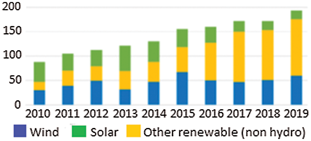
Figure 1: Annual installations of renewable energy plants in GW [1]
Neural network-based fault detection has been proposed for PV systems [12], but the study did not include a comparison of the detection algorithms for the purpose of determining which one was the best. Common PV array faults, such as open-circuit, short-circuit, degradation, and shading faults, were detected using thresholds of voltage and currents [13]. However, this method lacks accuracy when PV arrays receive continuously changing irradiation. In addition, faults that accumulate over time were not evaluated, and the presence of the protection diode makes fault detection in PV arrays difficult. Measurements of array voltages, currents, irradiance, and temperature were used to detect faults by computing the Thevenin equivalent resistance of the PV array [14]. Although a fault detection algorithm used a cross-correlation function to detect series arc faults, it did not examine shunt faults [15]. When the challenges of detecting line-to-line faults in PV systems were discussed, this fault detection method was restricted to the challenges of overcurrent protective relaying [16].
This study evaluates classification techniques according to their ability to detect several fault types that occur in PV systems in order to maintain continuity of renewable power service. A 250-kW PV power plant is simulated using MATLAB/Simulink to build the training and testing data of normal and abnormal plant conditions. The classification techniques are random forest, logistic regression, naive Bayes, AdaBoost, and CN2 rule induction. These were selected on the basis of their performance and accuracy. To achieve the best fault detection performance, the variables of the detection algorithm inputs are designed using training data measured from the PV farm during different fault cases. When it came to detecting PV faults, the AdaBoost algorithm was the most accurate of these detection and classification techniques.
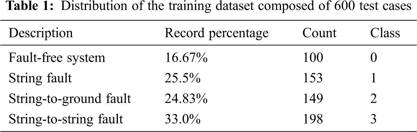
A simulated 250-kW PV power plant was utilized to create training and testing datasets of PV fault cases. The PV farm and its simulation are further discussed in Appendix A. Three fault types and normal operation (free-of-fault state) are defined. The default sets, as shown in Appendix A, are as follows. From the figure presented in the Appendix section, the fault cases F1, F2, and F3 describe a string fault (tested on string 1), string-to-ground fault (tested on string 1), and string-to-string fault (tested between strings 1 and 2), respectively. Training and testing datasets were built. The training dataset included 600 instances, each with 30 features and one column for classes or categories. Tab. 1 shows that the dataset included 100 (16.67%) free-of-fault cases, 153 cases (25.5%) of string faults, 149 cases (24.83%) of string-to-ground faults, and 198 cases (33%) of string-to-string faults. The total simulation time was 0.4 s, and a fault was assumed to occur at 0.2 s. In the training dataset, all measurements were taken after the fault occurred in the period from 0.2 s to 0.4 s. The testing dataset contained 50 instances. Measurements were taken in the period from 0.1 s to 0.3 s, with transient time from 0.1 s to 0.2 s, and faults occurring from 0.2 s to 0.3 s.
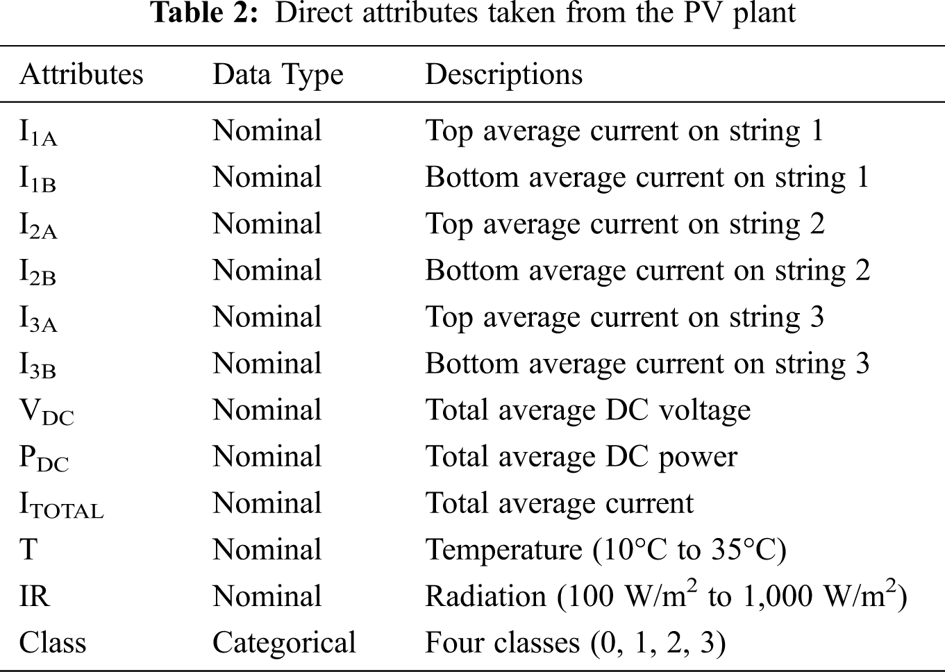
All features or attributes were random measurements of temperature, radiation, and fault resistance, ranging from 10°C to 35°C, 100 W/m2 to 1,000 W/m2, and 1 Ω to 2,000 Ω, respectively. The 30 features (or attributes) included the average, maximum, minimum, and variance values of the current from strings 1, 2, and 3. Tab. 2 shows that each string contained two ammeters to measure the current at its top and bottom during the simulation, and the directions of the two currents were the same. Other measurements, such as the total average DC power, total current, and total average DC voltage, were taken. Fault resistance and fault locations were not identified as a function by the proposed fault detection algorithms. Only the functions of fault detection and faulted string estimation are included in the proposed algorithm. The features that aided the most in enhancing accuracy are the following range values.
These range effects are discussed in the following section.
The dataset represents different features, such as categorical, numeric, and time. The ranking of attributes in the classified dataset considers the class-labeled datasets and scores attributes according to their correlation with the class. Tab. 3 describes the scoring methods (“Inf. Gain Ratio”), which is the expected amount of information (reduction of entropy). The gray rows in Tab. 3 show the top five rank attributes, Range3, Range4, Range2, Range1, and I2VAR, which are arranged according to rank. The table results show the main statistics for each attribute. The main tendency of the feature values is the mean value for numeric features and the mode for categorical features. The dispersion of the feature values for categorical features is the entropy of the value distribution, and for numeric features it is the coefficient of variation. The minimum and maximum values are computed for numerical and ordinal categorical features. The temperature T has values from 10°C to 35°C, with an average of 22.12°C. Radiation IR has values from 106 W/m2 to 1,000 W/m2, with an average of 552.20 W/m2. The total average current is 436.04 A, and the total average power is 141.32 kW.
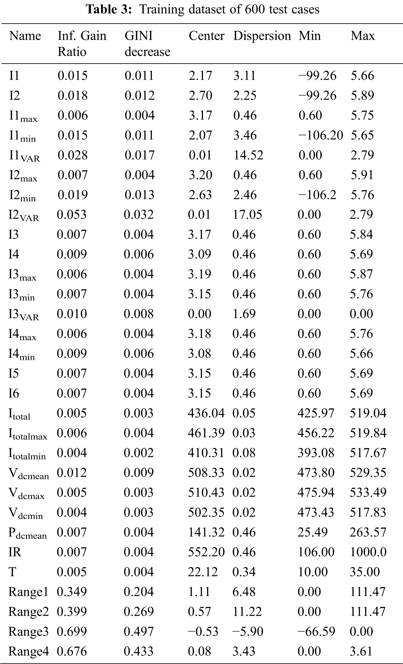
Fig. 2 shows the 2D visualization of classification trees. It consists of seven nodes and four leaves, with a depth of four levels and edge width relative to parents. At the top of Fig. 2 is Range3, which affects fault detection and classification by 33% at the first level. Range1 affects it by 60.5%, and the other ranges affect fault detection and classification by 57.1%.
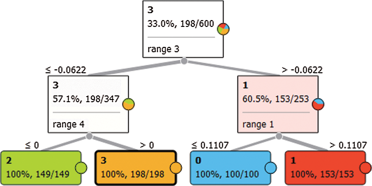
Figure 2: Visualization of the classification trees
We used five popular data mining algorithms for each dataset, using Orange, a machine learning and data mining platform suitable for data analyses that involve Python scripting and visual programming. The classification techniques predict a qualitative response by analyzing data and recognizing patterns. Many classification techniques or classifiers can be used. We chose the widely used naive Bayes [17–19], logistic regression (ridge and lasso) [20–23], random forest [24], AdaBoost [25], and CN2 rule induction [26,27]. Fig. 3 shows the proposed system model created on the Orange platform, with the five referenced models for PV fault detection and classification.
The 10-fold cross-validation method was applied to test the fault detection ability of the algorithms under study and to measure the unbiased estimate of our proposed models. In this cross-validation method, each dataset was randomly divided into a training set and a test set (i.e., 90% and 10% of the dataset, respectively). Accordingly, each set contained approximately the same percentage of samples of each class. The overall performance was obtained by determining the average for all 10 iterations.
The classification algorithm’s performance was evaluated according to the following factors:
• Precision and recall are two significant performance measures [28,29]. Precision is the ratio of the number of true positive assessments to the sum of all true and false positive assessments. Recall is the ratio of the number of true positive assessments to the number of all positive assessments.
• Classification accuracy (CA) is the ratio of the number of correct assessments to the number of all assessments [28,30].
• The F-measure combines recall and precision. It is the ratio of the product of precision and recall to their average [17,28].
• Specificity is the ratio of the number of true negative assessments to the number of all negative assessments [28].
• Log loss cross-entropy considers the uncertainty of fault detection on the basis of how much it varies from the actual label.
• Training time is the cumulative time in seconds used by a training model.
• The confusion matrix gives the number/proportion of instances between the predicted and actual class, so as to determine specific instances that are misclassified as well as how they are misclassified. The diagonal line in the confusion matrix contains all correctly classified instances, and the other values contain misclassified instances.
• The area under the receiver-operating curve (AROC) is for the tested models and the corresponding convex hull. It allows for the comparison of classification models. The curve plots a false-positive rate horizontally and a true-positive rate vertically. The closer the AROC is to unity, the more accurate the classifier. An AROC greater than 0.9 is excellent, 0.8 is good, 0.7 is nonsignificant, and anything lower than 0.7 is not good.
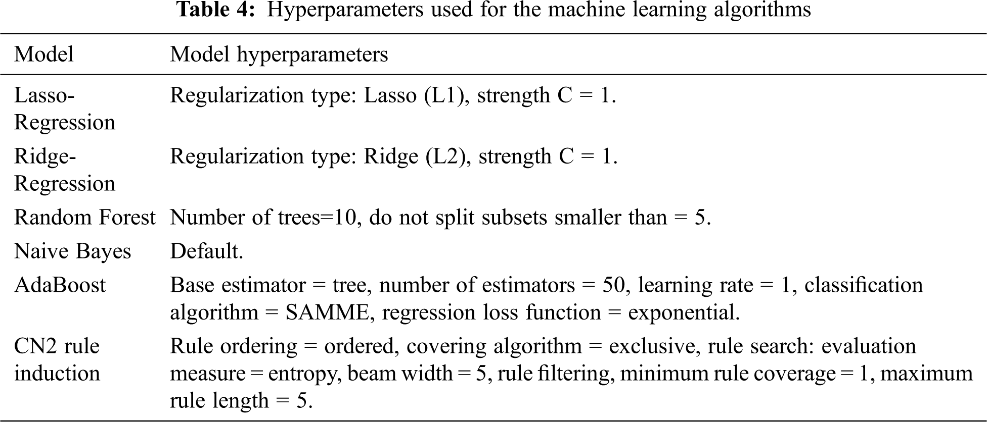
We designed the classifiers according to the hyperparameters listed in Tab. 4, so as to achieve the best performance of each classifier (“Model” in the table).
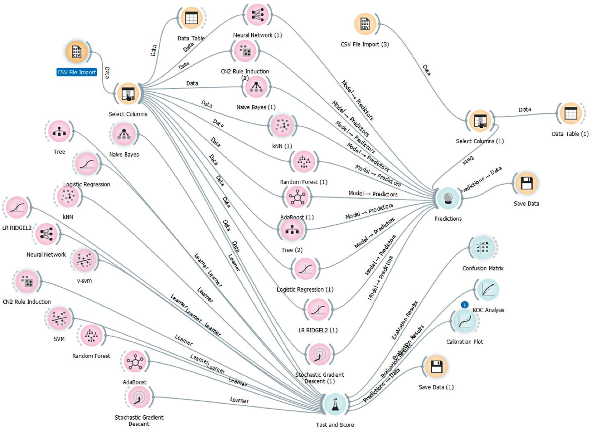
Figure 3: Proposed system model
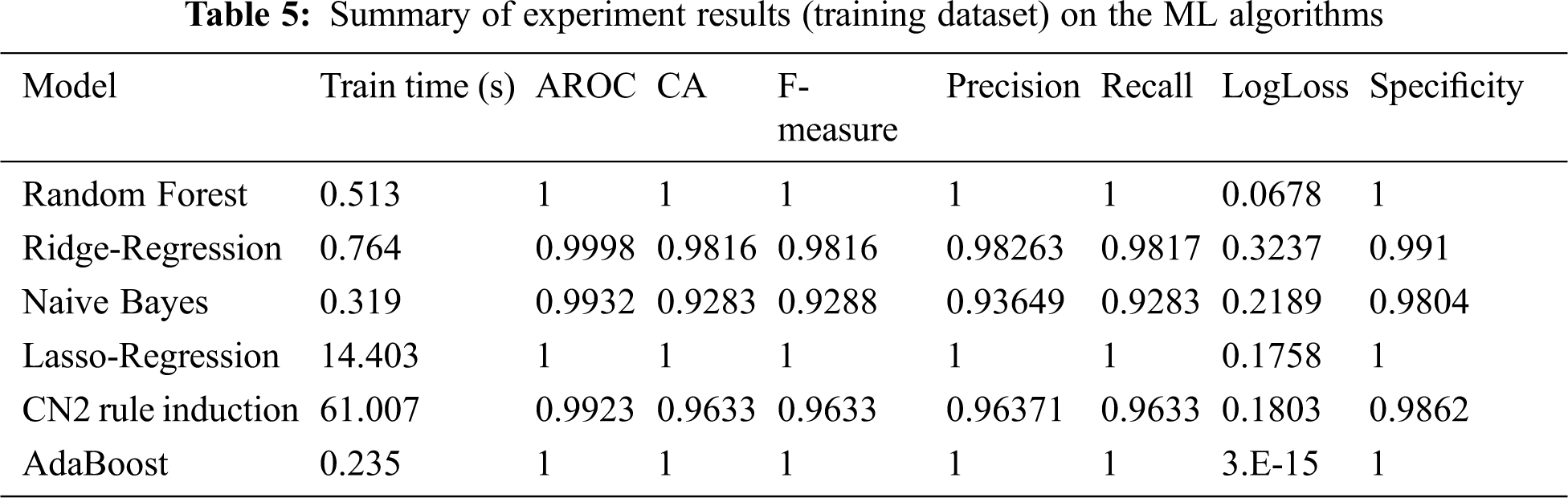
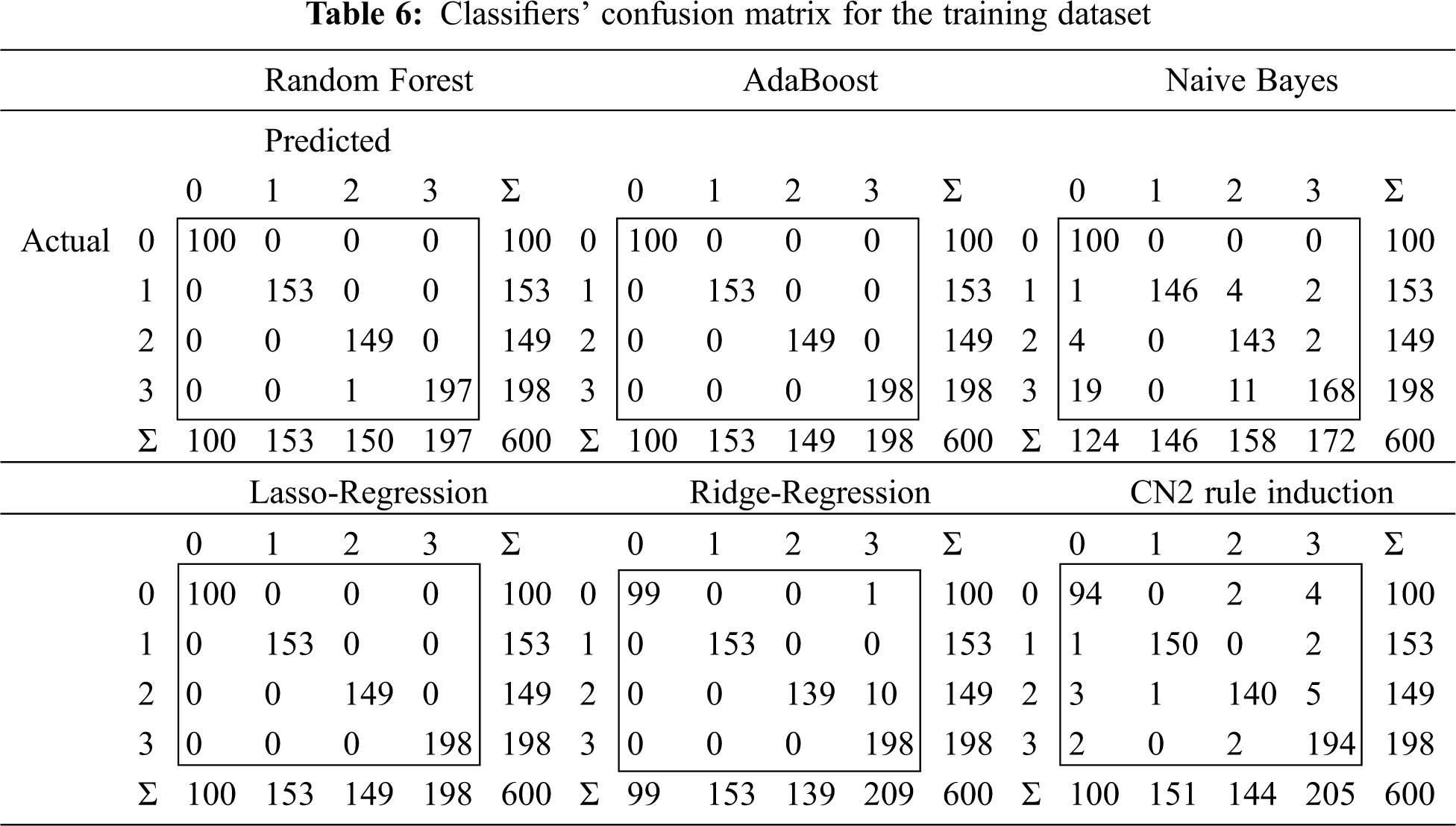
Tab. 5 summarizes the experimental results for the training dataset on the machine learning algorithms. The selected classifiers in general achieved good performance, with AdaBoost and random forest producing the best results. These two algorithms address an array of evaluation references of classification, such as training time, AROC, accuracy, F-measure, precision, recall, log loss, and specificity (see Tab. 5). The evaluations of these factors are close to one, except for log loss, which is close to zero. The training time values shown in Tab. 5 are low for most of the selected algorithms; the exception being the CN2 rule induction algorithm. The results shown in Tab. 6 confirm that AdaBoost and random forest yield the best performance. Tab. 6 summarizes the confusion matrix of each classifier for the training dataset. AdaBoost achieves the most broadly successful fault detection and classification for the training dataset, with 600 fault and free-of-fault test cases. Random forest succeeds in all cases except one: a single test case that is incorrectly identified, but detected as a fault case.
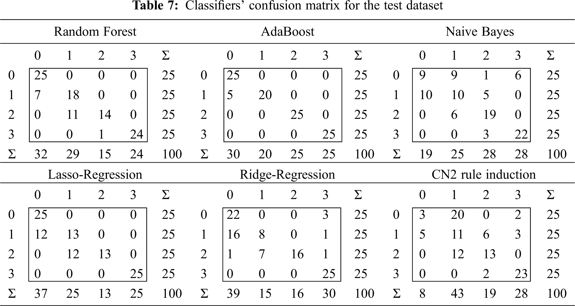
Tab. 7 shows the confusion matrix of the performance of each classifier in the testing dataset. AdaBoost exhibits the best performance in fault detection. Although five test cases were undetected, the algorithm successfully classified the detected fault cases. The five undetected fault cases were at high impedance, which is close to or greater than 500 Ω resistance and half the value of irradiation. Furthermore, these faults were in the same string (fault type) under the condition that the difference in voltage through the fault resistance was small. Accordingly, their fault currents were small, and the system behavior was close to the normal operation that limited fault detection. Furthermore, these five fault cases were not detected by the other classifiers, which had other undetected fault cases. AdaBoost, random forest, and lasso-regression successfully classified free-of-fault test cases. The other classifiers failed, as they incorrectly estimated the free-of-fault test cases as detected faults, where such operations are defined as loss of classifier security. AdaBoost showed the best performance at detecting faults, with successful identification of fault types. Therefore, AdaBoost is the only completely reliable algorithm for fault detection and classification.
Tab. 8 summarizes the performance of the algorithms in the test dataset according to the evaluation factors. AdaBoost performed best on the test dataset, with the highest values of AROC, CA, F-measure, precision, recall, and specificity, at 0.967, 0.95, 0.949, 0.958, 0.950, and 0.983, respectively. This confirms the superiority of AdaBoost as a fault classifier for PV plants.
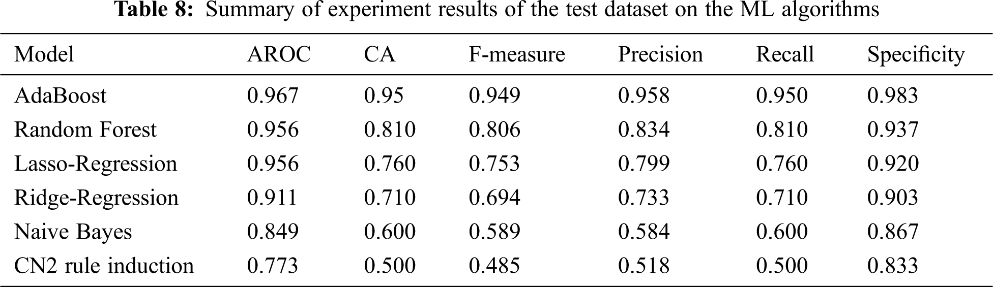
The ability of five algorithms to detect faults in PV plants was evaluated. These were based on six classifiers: random forest, ridge-regression, naive Bayes, logistic regression, CN2 rule induction, and AdaBoost. The fault dataset was obtained from the simulation of a 250-kW PV plant using Simulink/MATLAB. Of the six classifiers, CN2 rule induction exhibited the lowest performance in fault detection. The best performance was shown by AdaBoost, which could detect and indicate fault conditions such as string faults, string-to-ground faults, and string-to-string faults. Test results show that AdaBoost achieved the absolute highest values of AROC, CA, F-measure, precision, recall, and specificity, which were 0.967, 0.95, 0.949, 0.958, 0.950, and 0.983, respectively. Moreover, AdaBoost could achieve 100% fault detection despite the presence of fault cases with high resistance that produced a low level of current distribution changes. In general, AdaBoost performed successfully for training and testing fault cases, thereby confirming its efficacy.
Acknowledgement: The authors acknowledge the financial support received from Taif University Researchers Supporting Project (Number TURSP-2020/34), Taif University, Taif, Saudi Arabia. We thank LetPub (https://www.letpub.com) for its linguistic assistance during the preparation of this manuscript.
Funding Statement:Sherif S. M. Ghoneim is the author who received the financial grant from Taif University Researchers Supporting Project (Number TURSP-2020/34), Taif University, Taif, Saudi Arabia.
Conflicts of Interest:The authors declare that they have no conflict of interest.
1. International Energy Agency, “Photovoltaic power systems program, snapshot of global PV markets 2020,” Vol. 37, IEA-PVPS T1, 2020. [Google Scholar]
2. M. Khan, T. Malik and I. Sajjad, “A novel probabilistic generation model for grid connected PV based distributed generation,” Journal of Engineering Research, vol. 8, no. 1, pp. 231–247, 2020. [Google Scholar]
3. M. Rawat and S. H. Vadhera, “A comprehensive review on impact of wind and solar photovoltaic energy sources on voltage stability of power grid,” Journal of Engineering Research, vol. 7, no. 4, pp. 178–202, 2019. [Google Scholar]
4. M. Özçelik and A. Yilmaz, “Improving the performance of MPPT in PV systems by modified perturb-and-observe algorithm,” Journal of Engineering Research, vol. 3, no. 3, pp. 77–96, 2015. [Google Scholar]
5. K. Abdul Mawjood, S. H. S. Refaat and W. G. Morsi, “Detection and prediction of faults in photovoltaic arrays: A review,” in IEEE 12th Int. Conf. on Compatibility, Power Electronics and Power Engineering (CPE-POWERENG 2018Doha, Qatar, pp. 1–9, 2018. [Google Scholar]
6. M. Kh Alam, F. Khan, J. Johnson and J. Flicker, “A comprehensive review of catastrophic faults in PV arrays: Types, detection, and mitigation techniques,” IEEE Journal of Photovoltaics, vol. 5, no. 3, pp. 982– 997, 2015. [Google Scholar]
7. A. Mellit, G. M. Tina and S. A. Kalogirou, “Fault detection and diagnosis methods for photovoltaic systems: A review,” Renewable and Sustainable Energy Reviews, vol. 91, pp. 1–17, 2018. [Google Scholar]
8. I. M. Karmacharya and R. Gokaraju, “Fault location in ungrounded photovoltaic system using wavelets and ANN,” IEEE Trans. on Power Delivery, vol. 33, no. 2, pp. 549–559, 2018. [Google Scholar]
9. W. Fenz, S. Thumfart, R. Yatchak, H. Roitner and B. Hofer, “Detection of arc faults in PV systems using compressed sensing,” IEEE Journal of Photovoltaics, vol. 10, no. 2, pp. 676–684, 2020. [Google Scholar]
10. B. T. P. Sh.Lu,D.Zhang, “A comprehensive review on DC arc faults and their diagnosis methods in photovoltaic systems,” Renewable and Sustainable Energy Reviews, vol. 89, pp. 88–98, 2018. [Google Scholar]
11. R. Fazai, K. Abodayeh, M. Mansouri, M. Trabelsi and G. E. Georghiou, “Machine learning-based statistical testing hypothesis for fault detection in photovoltaic systems,” Solar Energy, vol. 190, no. 3, pp. 405–413, 2019. [Google Scholar]
12. M. Hussain, M. Dhimish, S. Titarenko and P. Mather, “Artificial neural network based photovoltaic fault detection algorithm integrating two bi-directional input parameters,” Renewable Energy, vol. 155, no. 3, pp. 1272–1292, 2020. [Google Scholar]
13. T. Pei and X. Hao, “A fault detection method for photovoltaic systems based on voltage and current observation and evaluation,” Energies, vol. 12, pp. 1–16, 2019. [Google Scholar]
14. B. K. Karmakar and A. K. Pradhan, “Detection and classification of faults in solar PV array using Thevenin equivalent resistance,” IEEE Journal of Photovoltaics, vol. 10, no. 2, pp. 644–654, 2020. [Google Scholar]
15. M. Ahmadi, H. Samet and T. Ghanbari, “Series arc fault detection in photovoltaic systems based on signal-to-noise ratio characteristics using cross-correlation function,” IEEE Trans. on Industrial Informatics, vol. 16, no. 5, pp. 3198–3209, 2020. [Google Scholar]
16. Y. Zhao, J. Palma, J. Mosesian, R. Lyons and B. Lehman, “Line-line fault analysis and protection challenges in solar photovoltaic arrays,” IEEE Trans. on Industrial Electronics, vol. 60, no. 9, pp. 3784– 3795, 2013. [Google Scholar]
17. H. Chaudhary, K. Kohli, S. Amin, P. Rathee and V. Kumar, “Optimization and formulation design of gels of Diclofenac and Curcumin for transdermal drug delivery by Box-Behnken statistical design,” Journal of Pharmaceutical Sciences, vol. 100, no. 2, pp. 580–593, 2011. [Google Scholar]
18. S. Raschka, “Naïve Bayes and text classification I-introduction and theory,” arXiv preprint arXiv:1410.5329, 2014. [Google Scholar]
19. N. Friedman, D. Geiger and M. Goldszmidt, “Bayesian network classifiers,” Machine Learning, vol. 29, no. 2/3, pp. 131–163, 1997. [Google Scholar]
20. D. G. Kleinbaum, K. Dietz, M. Gail, M. Klein and M. Klein, Logistic Regression. New York: Springer-Verlag, 2002. [Google Scholar]
21. S. Menard, “Applied logistic regression analysis,” Sage, London, UK, 2nd Edition. vol. 106, pp. 67–90, 2001. [Google Scholar]
22. A. Jaokar, “Logistic regression as a neural network,” Data Science Central, 2019. [online]. Available: https://www.datasciencecentral.com/profiles/blogs/logistic-regression-as-a-neural-network. [Google Scholar]
23. A. Subasi and E. Ercelebi, “Classification of EEG signals using neural network and logistic regression,” Computer Methods and Programs in Biomedicine, vol. 78, no. 2, pp. 87–99, 2005. [Google Scholar]
24. M. Pal, “Random forest classifier for remote sensing classification,” Int. Journal of Remote Sensing, vol. 26, no. 1, pp. 217–222, 2007. [Google Scholar]
25. R. E. Schapire, Y. Freund, P. Bartlett and W. S. Lee, “Boosting the margin: A new explanation for the effectiveness of voting methods,” Annals of Statistics, vol. 26, no. 5, pp. 1651–1686, 1998. [Google Scholar]
26. P. Clark and T. Niblett, “The CN2 induction algorithm,” Machine Learning, vol. 3, no. 4, pp. 261–283, 1989. [Google Scholar]
27. P. Clark and R. Boswell, “Rule induction with CN2: Some recent improvements,” Proc. European Working Session on Learning, Berlin, vol. 482, pp. 151–163, 1998. [Google Scholar]
28. A. Tharwat, “Classification assessment methods,” Applied Computing and Informatics, pp. 2–13, 2018. [Google Scholar]
29. K. J. Cios, W. Pedrycz and R. W. Swiniarski, “Data mining and knowledge discovery,” in Data mining methods for knowledge discovery, Boston, MA: Springer, pp. 1–26, 1998. [Google Scholar]
30. J. Han, M. Kamber and J. Pei, “Data mining: Concepts and Techniques,” Waltham, MA: Morgan Kaufmann, 2012. [Google Scholar]
Fig. A1 shows the simulated PV power system created using Simulink/MATLAB. Fig. A1(a) shows that it is grid-connected by a three-level inverter. The inverter is an IGBT bridge that is PWM-controlled. The inverter control was designed to implement the maximum power point tracking of the PV system based on the perturbation and observation approach. As depicted in the Simulink circuit in Fig. A1(b), a three-phase 0.25/250-kV power transformer was used to interconnect the PV system with the electric power grid. The grid domain had two short transmission lines. The first line was 14 km long and directed to the 120-kV power equivalent grid through a power transformer. The second line was an 8-km feeder directed to a static load. As depicted in Fig. A1(c), the PV system contained 88 parallel strings, each involving seven series modules. Each module had 128 cells, a maximum power of 414.801 W at 72.9 V, current of 5.69 A, open-circuit voltage of 85.3 V, and short-circuit current of 6.09 A.
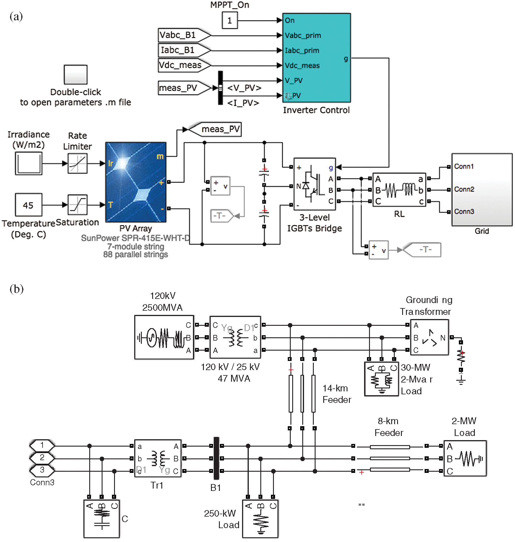
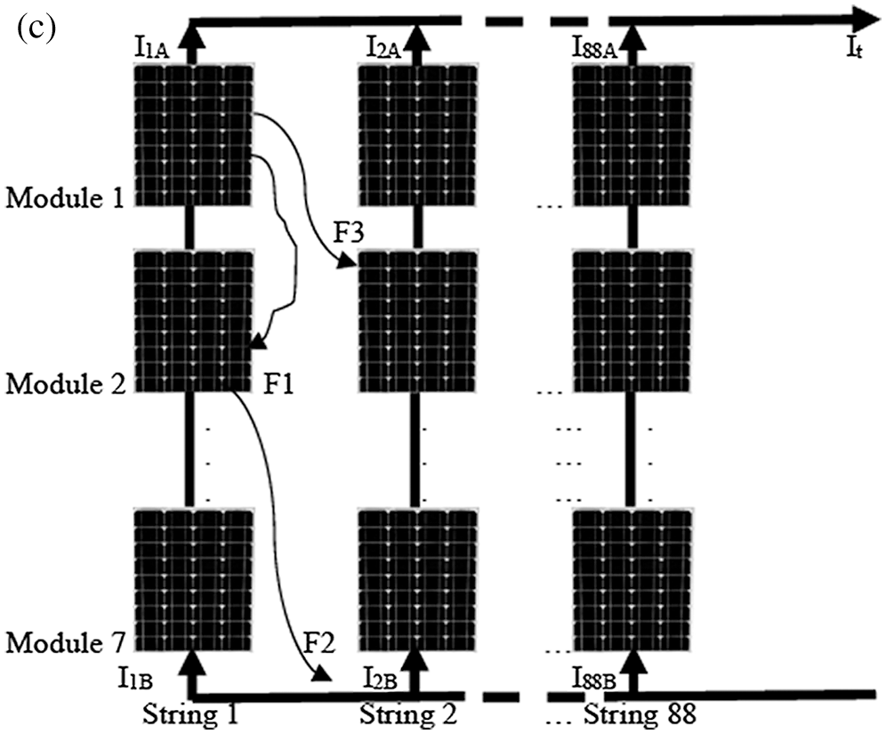
Figure A1: Diagram of the grid-connected PV simulated system. a. Schematic of the grid-connected PV panel created using MATLAB/Simulink b. MATLAB/Simulink circuit of the power grid c. Matrix allocation of the PV power farm
 | This work is licensed under a Creative Commons Attribution 4.0 International License, which permits unrestricted use, distribution, and reproduction in any medium, provided the original work is properly cited. |