DOI:10.32604/iasc.2021.018607
| Intelligent Automation & Soft Computing DOI:10.32604/iasc.2021.018607 | |
| Article |
Breast Cancer Classification Using Deep Convolution Neural Network with Transfer Learning
Department of Computer Sciences, College of Computer and Information Sciences, Princess Nourah bint Abdulrahman University, Riyadh, 11047, KSA
*Corresponding Author: Hanan A. Hosni Mahmoud. Email: hahosni@pnu.edu.sa
Received: 13 March 2021; Accepted: 18 April 2021
Abstract: In this paper, we aim to apply deep learning convolution neural network (Deep-CNN) technology to classify breast masses in mammograms. We develop a Deep-CNN combined with multi-feature extraction and transfer learning to detect breast cancer. The Deep-CNN is utilized to extract features from mammograms. A support vector machine (SVM) is then trained on the Deep-CNN features to classify normal, benign, and cancer cases. The scoring features from the Deep-CNN are coupled with texture features and used as inputs to the final classifier. Two texture features are included: texture features of spatial dependency and gradient-based histograms. Both are employed to locate breast masses in mammograms. Next we apply transfer learning to the classifier of the SVM. Four techniques are devised for the experimental evaluation of the proposed system. The fourth technique combines the Deep-CNN with texture features and local features extracted by the scale-invariant feature transform (SIFT) algorithm. Experiments are designed to measure the performance of the various techniques. The results demonstrate that the proposed CNN coupled with the texture features and the SIFT outperforms the other models and performs best with transfer learning embedded. The accuracy of this model is 97.8%, with a true positive rate of 98.45% and a true negative rate of 96%.
Keywords: Breast cancer; Classification; Neural network; Texture features; Transfer learning
Breast cancer is one of the most common cancers in the female population. Over two million women are affected by breast cancer each year. Breast cancer is a severe illness that affects the breast tissues and can spread to nearby organs [1]. The American Cancer Society published data of 277,580 invasive cases and 48,640 non-invasive cases of breast cancer in 2020 [2].
The death rate is very high for patients with breast cancer, so women over age of forty are advised to undergo mammogram screening regularly [3]. Mammography is utilized as an imaging tool for breast tumor examination because it allows for a precise diagnosis even in the early stages of cancer. Early discovery is important to advance the breast cancer diagnosis rate and improve the chances of recovery [4]. The wide utilization of mammography-based diagnosis can discover asymptomatic breast cancer, which can lead to a reduced mortality rate from this disease [5]. Radiologists look for essential properties such as microscopic calcifications and tissue distortions, which designate the presence of breast cancer [6].
Masses found in breast mammograms are important indications of malignant breast tumors [7]. Tumor recognition is a difficult job because of the subtle differences between tumor tissue and adjacent healthy tissues [8]. Mass discovery in the breast, that is, locating boundaries between mass and healthy regions, is also difficult [9] due to low-quality images and high ratios of noise [10]. In addition, the resemblance of masses with the adjacent healthy regions is high [11]. However, identifying the tumor shape and type is vital to proper diagnosis [12]. These problems lead to less-than-optimal sensitivity and specificity of mammogram screening [13]. Additionally, the inspection procedure of mammograms is tiresome and can be biased [14].
Therefore, several computer-aided diagnosis and image analysis tools are used by medical experts to increase diagnosis correctness. These tools employ feature extraction and heuristic techniques [15]. Then classifiers utilize the extracted features to differentiate masses from normal tissues [16]. Feature extraction relies heavily on geometrical and morphological properties. Computerized tools can enhance identification of suspicious masses and other abnormalities, such as calcifications, through learning methods [17]. Several previous studies described various approaches for computerized detection of abnormalities in mammograms [18]. For example, the authors in Giger et al. [19], regions of interest were segmented as suspicious areas and classified utilizing texture features through linear discriminant analysis. The main problems facing such approaches are the noises included in the images and the size, texture, and appearance variations of breast tumors [20].
The performance of breast cancer automated diagnosis can be enhanced using deep learning methods [21]. Machine learning techniques can be used for identifying features as representatives [22]. Texture also can be utilized through identifying local statistical aspects of image intensity maps [23]. Texture analysis techniques can be used in analyzing lesions instigated by masses in mammograms and can differentiate masses and normal tissues [24].
In Oliver et al. [7], the authors extracted texture features from breast suspected regions via fuzzy C-means algorithm. In Chen et al. [25] the authors modeled tissue patterns in mammograms using tissue appearances.
Deep learning techniques require medical image analysis CAD tools [26–29]. Classification processes can utilize statistical methods, artificial intelligence techniques, or support vector machines (SVM) to predict breast cancer [30]. Deep learning approaches can be used to generate semantic information through adaptive learning [31,32].
CNN can classify masses from breast mammograms by extracting texture features. The textural topographies are fed as inputs to a CNN classifier [33]. However, texture features are not adequate to classify cancer masses from mammograms. Therefore, morphological features of the tumor shape are also utilized in categorizing cancer masses.
In this paper, we present a Deep-CNN method for feature extraction of three kinds of breast cancer masses. Multiple properties of the gray level co-occurrence matrix (GLCM) and the histogram of oriented gradient (HOG) [34,35] are examined to emphasize the texture features of the region of interest (ROI). Texture scoring features analogous to each breast mammogram are pooled into multi-features. The pooled features are presented to diverse numbers of classifiers and grouped into the anticipated classes. We utilize the SVM classification algorithm to define the ROI as normal, benign tumor, or cancer [36–38]. The proposed system is composed of three main phases: feature extraction, texture extraction, and tumor classification.
In this section, we will describe the dataset used and the methodology.
We utilize the dataset in the digital database of mammography in Nascimento et al. [39]. The dataset consists of mammography from 2200 cases. Each mammogram has clinical data such as shapes, sizes, and densities of the breast masses as well as diagnoses annotated by radiologists [40–43].
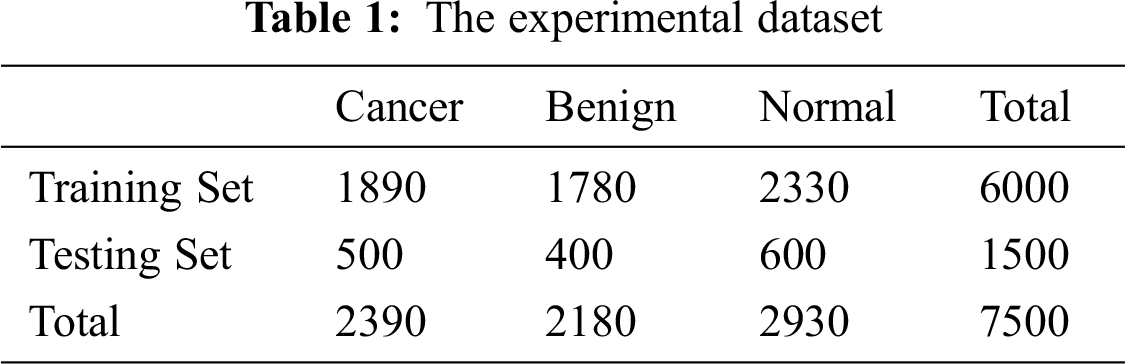
Mammograms in the dataset include the pectoral muscle and the background, both of which include many artifacts. The classification is performed only on ROIs that might contain abnormalities. The ROI has to cover the whole abnormality and minimal normal tissue surrounding the abnormality. Mammograms are cropped, and the parts that affect classification are removed. A simulation study of extracting ROIs from mammograms in the dataset is conducted. The extracted ROIs include benign and cancer masses following the process in [44–46]. The data are partitioned into a training set and a testing set with the proportions of 80% and 20%, respectively, as depicted in Tab. 1.
The experimental dataset is composed of 7500 images. The training set contains 6000 images, among which 1890 are cancer, 1780 are benign, and 2330 are normal. Random selections of 500 cancer regions, 400 benign regions, and 600 normal regions are designated for training. The selected regions are selected from different mammograms of different cases to avoid data bias.
The Inception module is utilized for the first time in GoogLeNet [47]. This module approximates an optimal sparse configuration in a CNN by utilizing dense components [48]. It searches for the optimal local configuration and duplicates it, building a multi-layer network from the convolutional network blocks.
In Arora et al. [49], the authors reported that every unit from the previous layer represents an input image region, and they concluded that these units are assembled in filter stores. Correlated units in lower layers focus on local regions and can be used as inputs to convolutions layers of 1*1 in the succeeding layer [50]. If Smaller clusters are enclosed within larger regions, the convolutions will ignore those larger regions. Spatially spread smaller clusters are enclosed by convolutions over patches with larger regions, and the convolutions will ignore larger region patches. To avoid such problems, the Inception architecture is limited to filter sizes of 1*1, 3*3, and 5*5. For better results, the authors added pooling layers with alternative path [51,52].
Adding parallel pooling layers can result in a high cost, especially when there are convolutional layers with many filters. When pool layers are supplemented, the cost becomes more problematic. Even with the architecture covering the optimal structure, it is highly inefficient and can result in a huge computational cost in few stages. Dimension reduction can be applied to reduce the computational cost. In one study, the author suggested using (1*1) convolutions instead of (3*3) or (5*5) convolutions to reduce the computational cost [47].
Some authors suggested factorizing filters into smaller ones. Utilizing asymmetric convolutions (n∗1) can offer better performance than symmetric convolutions. In Fedorov et al. [53], the authors described an (n∗1) convolution trailed by a (1∗n) convolution and found out that it can be equal to a two-layer convolution equivalent to an (n∗n) convolution as shown in Fig. 1. The cost of the two-layer convolution is 33% less compared to the equivalent output filters. It is proved that a (1∗n) convolution trailed by an (n∗1) convolution can replace the (n∗n) solution with significant cost savings.
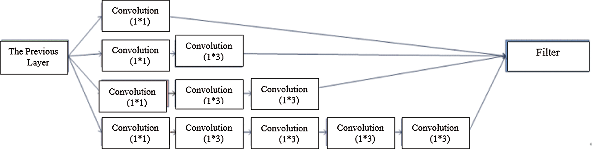
Figure 1: Asymmetric convolutions
2.3.1 Texture Features of Spatial Dependency (TFSD)
Texture features are often utilized to identify objects in an image. This is considerably helpful for breast cancer diagnosis because breast masses have different shapes in mammography. Mass edges can define the type of breast cancer as well as its degree. The length of the edge is long, and the different lumps develop irregular texture features that resemble a definite type of mass. We develop a technique to classify masses in mammograms by identifying texture features utilizing spatial dependency (TFSP). TFSP is calculated from pixel pairs with specific frequencies and spatial associations.
In Fig. 2, a spatial cell has four nearest spatial cells in the vertical and horizontal directions. Texture is indicated by a gray intensity matrix (GIM) F, where Fi,j represents a relative frequency. Fi,j represents two spatial cells parted by a displacement d on the image: one is of gray intensity i, and the other is of gray intensity j. The GIM is a function of the angle between the resolution of the neighboring cells and the distance between them (Fi,j (d,0); Fi,j (d,90)).
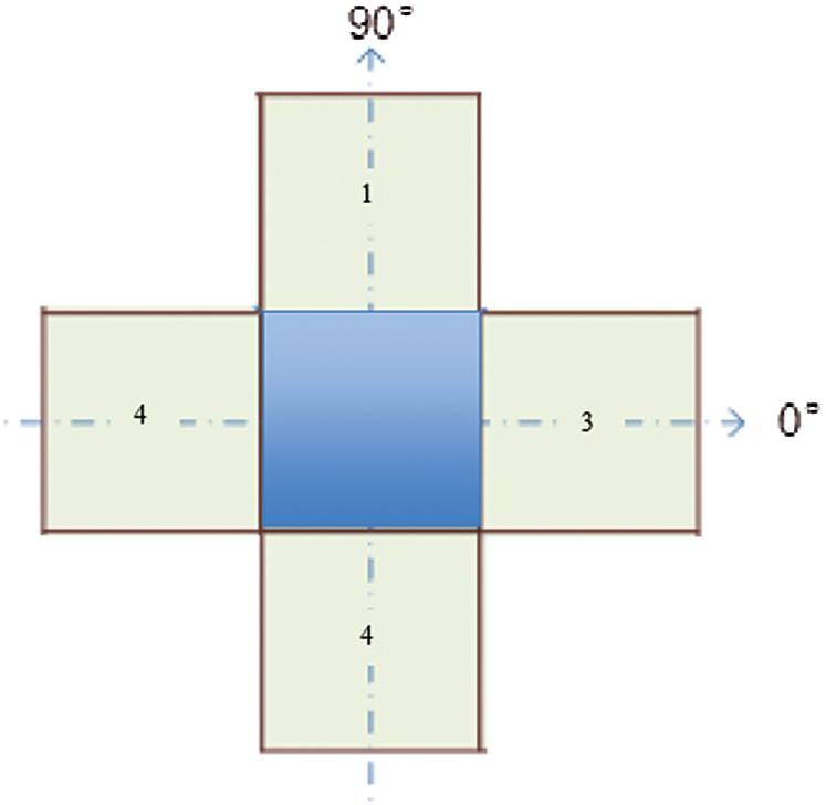
Figure 2: A cell with four spatial neighbors in two directions
We compute the features of each element from elements of the GIM. The GIM’s first two features are the mean and standard deviation of various angles. The other features are correlation and homogeneity. These features are functions of angle and distance. If image I has features X and Y at angles of 0° and 90° (as depicted in Fig. 2), the features will be represented by the functions of X and Y, along with their mean and variance. These features will be utilized as the classifier’s inputs.
The correlation, C, is the gray intensity in the image and is calculated with Eq. (1).
where μi and μj represent the means of Fi,j, while σi and σj represent the standard deviations of Fi,j.
Homogeneity, H, is the distance difference of the texture of the image. H is a metric of the local change of the texture and is defined in Eq. (2).
2.3.2 Gradient-Based Histogram
The gradient-based histogram has the ability to describe features such as object local structure, extract accurate gradient and edge information, and calculate the horizontal as well as the vertical gradients of an image. The algorithm partitions the image into units of equal size. For each cell, the histogram is computed as a representation of relative pixel intensity. The image is partitioned into 8 × 8 non-overlapping pixel units. For each unit, we compute the histogram in the direction of the pixels’ gradient. Depending on the gradient at that pixel, four (2 × 2) block units will be utilized to normalize the histogram of a given unit to be adapted to the energy in each of these block units.
Experiments are designed to evaluate the abilities of our methodology to detect breast cancer tumors and classify them in the selected dataset [39]. A Deep-CNN network combined with transfer learning and a Deep-CNN combined with SVM are tested for their ability to enhance the classifier performance. The main function of the classifier is to classify an ROI as normal, benign, or cancer.
Technique 1 (T1): The Deep-CNN is designed to be coupled with transfer learning. The CNN is trained with the mammogram datasets (DS) with previous transfer learning from ImageNet. The performance of the classifier is tested by inputting images into the Deep-CNN via runs of convolution, pooling, and classification layers. This technique is designed to evaluate the classification ability of Deep-CNN with transfer learning. The block diagram of T1 is shown in Fig. 3.

Figure 3: The Deep-CNN combined with transfer learning (T1)
Technique 2 (T2): The Deep-CNN is designed to be combined with transfer learning (TF) and SVM. The CNN is trained with the mammogram datasets. The classifier score is the output feature vector through inputting images into the SVM for training. This technique is designed to compare the classification abilities with and without transfer learning. The block diagram of T2 is shown in Fig. 4.

Figure 4: The Deep-CNN combined with transfer learning and SVM score (T2)
Technique 3 (T3): This technique utilizes texture to identify ROI in the mammogram image. The texture features are computed using texture features of spatial dependency (TFSD) and gradient-based histogram (GBH). This technique evaluates the classifier ability without learning transfer. The texture features are computed from the ROI from the dataset DS and are used for the training of the Deep-CNN. The block diagram of T3 is shown in Fig. 5.
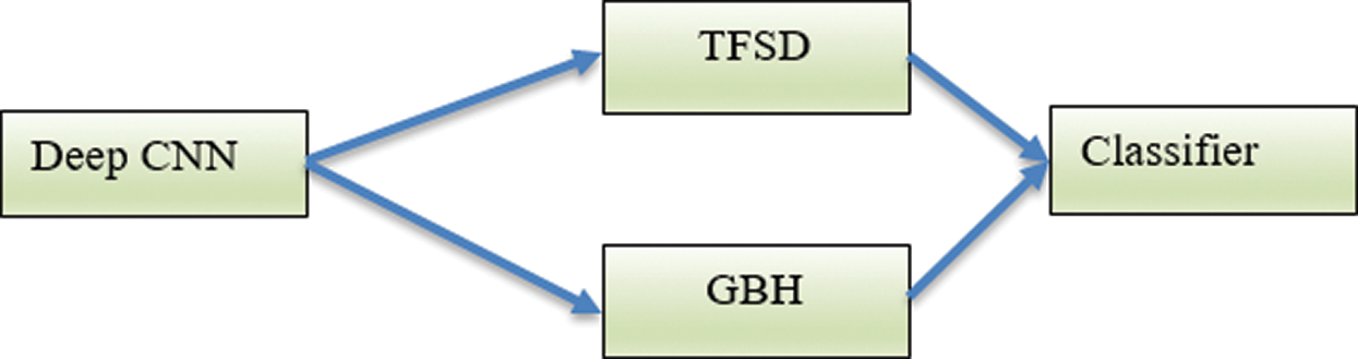
Figure 5: The Deep-CNN using the texture features TFSD and GBH (T3)
Technique 4 (T4): This technique integrates the technique in T3 with the SIFT local features. The integrated features are used as input vectors into the SVM machine. The block diagram of T4 is shown in Fig. 6.
Fig. 7 depicts a mammogram image of a breast with normal tissues from the dataset DS, while Fig. 8 depicts a mammogram image from the DS dataset with cancer ROI that has been detected using T3. In Fig. 9, a mammogram is shown after applying texture features coupled with SIFT local features using T4.
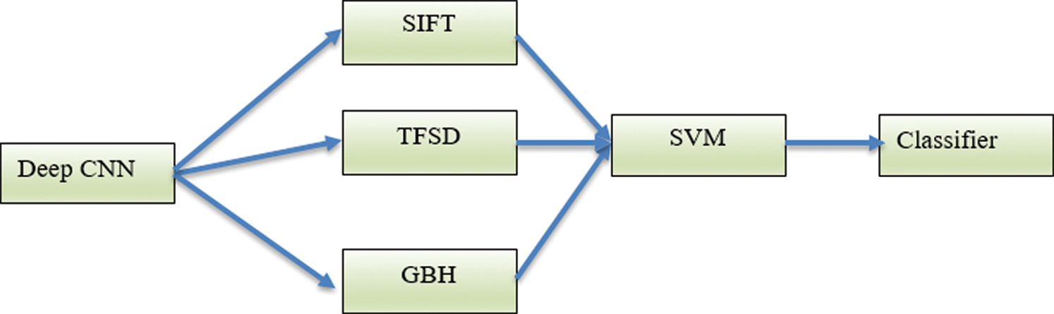
Figure 6: The Deep-CNN using the texture features TFSD and GBH coupled with SIFT local features (T4)
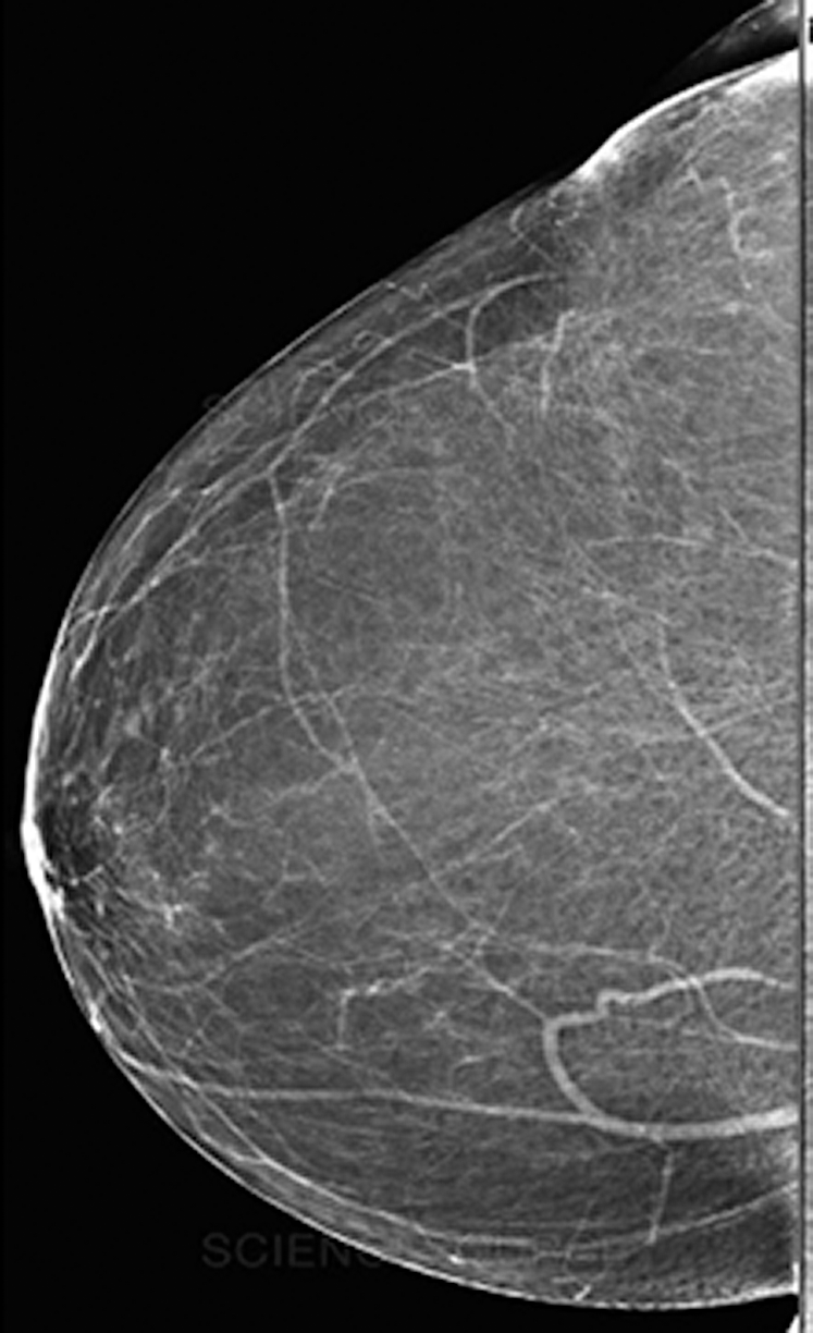
Figure 7: A mammogram image of a breast with normal tissues
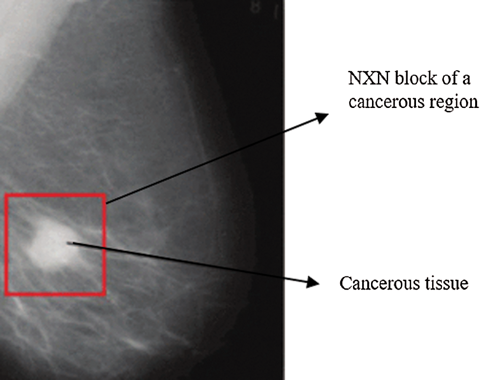
Figure 8: A mammogram image from the DS dataset with cancer ROI using T3
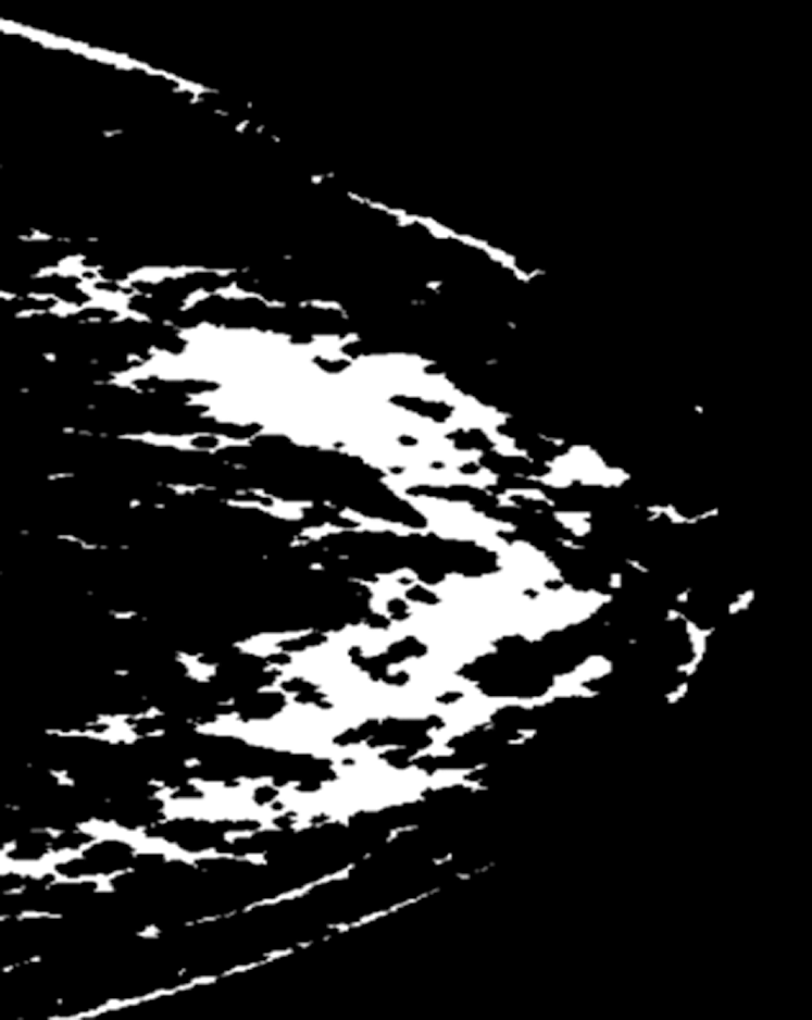
Figure 9: A mammogram after applying texture features coupled with SIFT local features using T4
The Deep-CNN network classifies breast mammogram ROIs as cancer, benign, or normal. Utilizing the Softmax layer, the evaluation of the classifier performance is defined as the capability of the classifier to correctly detect the breast region type [54]. We utilize the accuracy, sensitivity, and specificity metrics to measure the four classification techniques described in Section 3.
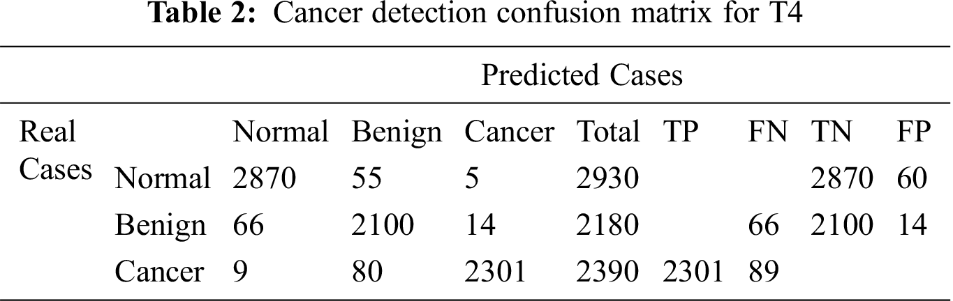
The confusion matrix for T4 is illustrated in Tab. 2. The results of medical diagnosis with the classifier described in T4 are depicted. Our proposed technique T4 is shown to have the capability to classify three types of breast ROI mammogram images as normal, benign, or cancer.
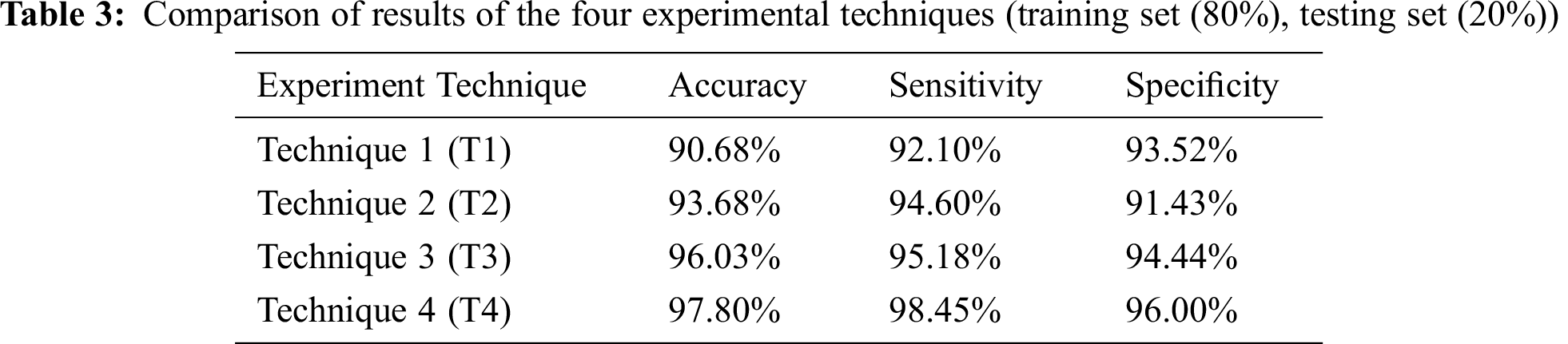
The four techniques are then compared according to the chosen accuracy metrics in Tab. 3.
The Deep-CNN classifier in the defined four techniques, T1 through T4, is assessed using the accuracy, sensitivity, and specificity metrics, as depicted in Eqs. (3)–(5), respectively.
TP, TN, FP, and FN indicate true positive, true negative, false positive, and false negative cases, respectively. Sensitivity indicates the true positive rate, and Specificity indicates the true negative rate.
Tab. 3 depicts the comparison of results of the four experimental techniques adopted in this research. The k-Fold Cross-Validation testing method is used, where the training set is 80% and the testing set is 20% of the whole dataset.
4.2 Results of Transfer Learning
In this section, we will discuss the impact of transfer learning on the performance of the different classifiers enhanced by T1 through T4.
The Deep-CNN with transfer learning provides much better classification accuracy and sensitivity than the same Deep-CNN without transfer learning. Figs. 10 and 11 show the comparison of the four techniques (T1 through T4) with and without transfer learning with an epoch of 100,000 and 200,000.
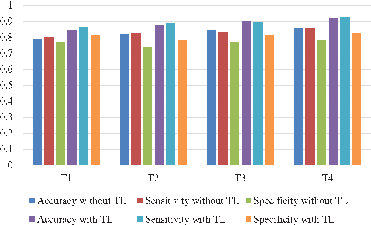
Figure 10: Comparison of accuracy and sensitivity of techniques T1 through T4 with and without transfer learning (TL) with epoch 100,000
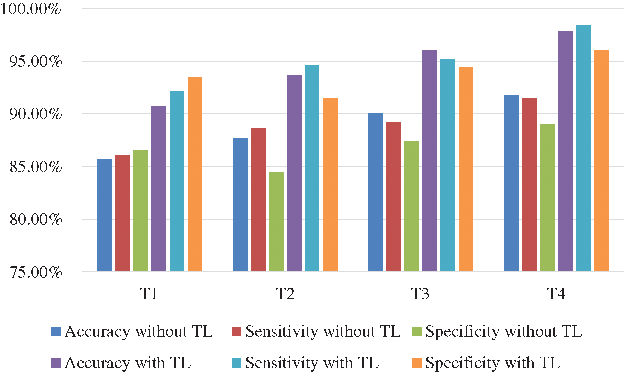
Figure 11: Comparison of accuracy and sensitivity of techniques T1 through T4 with and without transfer learning (TL) with epoch 200,000
In our research, we proposed a classification method for breast ROI tumors into normal, benign and cancerous classes. We utilized mammograms where ROI are classified using several features through suggesting four techniques coupled with Deep-CNN. Our study indicated that using several features in a model would outperform models with single feature. We coupled our Deep-CNN with transfer learning in the proposed four techniques. Transfer learning helped the model to achieve higher accuracy than without transfer learning. Features were extracted and are used as an input to the Deep-CNN which. Our proposed method integrated the Deep-CNN with texture features and SIFT local features. SVM is used in the training phase on the Deep-CNN features to classify breast masses. The features from the Deep-CNN are combined with texture features and used in the final classifier. We applied transfer learning to the classifier of the SVM. We devised four techniques for the experimentation of the proposed system. The fourth technique combined all the featured suggested in this research. It combined the Deep-CNN with texture features and local features extracted by the scale-invariant feature transform (SIFT) algorithm. Experiments were designed to measure the performance of the various techniques. The results demonstrated that the proposed CNN coupled with the texture features and the SIFT outperforms the other models and performs the best results with the transfer learning embedded. The accuracy of this model is 97.8%, with true positive rate of 98.45% and true negative rate of 96%.
Funding Statement: This research was funded by the Deanship of Scientific Research at Princess Nourah bint Abdulrahman University through the Fast-track Research Funding Program.
Conflicts of Interest: The authors declare that they have no conflicts of interest to report regarding the present study.
1. R. L. Siegel, K. D. Miller and A. Jemal, “Cancer statistics 2017,” CA: A Cancer Journal for Clinicians, vol. 67, no. 1, pp. 7–30, 2017. [Google Scholar]
2. E. A. Sickles, “Breast cancer screening outcomes in women ages 40-49: Clinical experience with service screening using modern mammography,” JNCI Monographs, vol. 1997, no. 22, pp. 99–104, 1997. [Google Scholar]
3. J. S. Whang, S. R. Baker, R. Patel, L. Luk and A. Castro, “The causes of medical malpractice suits against radiologists in the United States,” Radiology, vol. 266, no. 2, pp. 548–554, 2013. [Google Scholar]
4. M. Elter and A. Horsch, “CADx of mammographic masses and clustered microcalcifications: A review,” Medical Physics, vol. 36, no. 1, pp. 2052–2068, 2009. [Google Scholar]
5. R. M. Rangayyan, S. Banik and J. E. L. Desautels, “Computer-aided detection of architectural distortion in prior mammograms of interval cancer,” Journal of Digital Imaging, vol. 23, no. 5, pp. 611–631, 2010. [Google Scholar]
6. L. T. Niklason, D. B. Kopans and L. M. Hamberg, “Digital breast imaging: Tomosynthesis and digital subtraction mammography,” Breast Disease, vol. 10, no. 3-4, pp. 151–164, 1998. [Google Scholar]
7. A. Oliver, J. Freixenet, R. Marti, J. Pont, E. Perez et al., “A novel breast tissue density classification methodology,” IEEE Transactions of Information Technology Biomedical, vol. 12, no. 1, pp. 55–65, 2008. [Google Scholar]
8. A. Oliver, M. Tortajada, X. Lladó, J. Freixenet, S. Ganau et al., “Breast density analysis using an automatic density segmentation algorithm,” Journal of Digital Imaging, vol. 28, no. 5, pp. 604–612, 2015. [Google Scholar]
9. A. Rampun, B. Scotney, P. Morrow, H. Wang and J. Winder, “Breast density classification using local quinary patterns with various neighbourhood topologies,” Journal of Imaging, vol. 4, no. 1, pp. 14, 2018. [Google Scholar]
10. L. J. Warren, “Variability in interpretive performance at screening mammography and radiologists’ characteristics associated with accuracy,” Breast Diseases: A Year Book Quarterly, vol. 21, no. 4, pp. 330–332, 2010. [Google Scholar]
11. B. W. Hong and B. S. Sohn, “Segmentation of regions of interest in mammograms in a topographic approach,” IEEE Transactions of Information Technology Biomedical, vol. 14, no. 1, pp. 129–139, 2010. [Google Scholar]
12. J. Tang, R. M. Rangayyan, J. Xu, I. El Naqa and Y. Yang, “Computer-aided detection and diagnosis of breast cancer with mammography: Recent advances,” IEEE Transactions of Information Technology Biomedical, vol. 13, no. 2, pp. 236–251, 2009. [Google Scholar]
13. J. J. Fenton, J. Egger, P. A. Carney, G. Cutter, C. D’Orsi et al., “Reality check: Perceived versus actual performance of community mammographers,” American Journal of Roentgenology, vol. 187, no. 1, pp. 42–46, 2006. [Google Scholar]
14. C. W. Huo, G. L. Chew, K. L. Britt, W. V. Ingman, M. A. Henderson et al., “Mammographic density—A review on the current understanding of its association with breast cancer,” Breast Cancer Research and Treatment, vol. 144, no. 3, pp. 479–502, 2014. [Google Scholar]
15. W. A. Berg, C. Campassi, P. Langenberg and M. J. Sexton, “Breast imaging reporting and data system: Inter- and intraobserver variability in feature analysis and final assessment,” American Journal of Roentgenology, vol. 174, no. 6, pp. 1769–1777, 2000. [Google Scholar]
16. F. Winsberg, M. Elkin, J. Macy, V. Bordaz and W. Weymouth, “Detection of radiographic abnormalities in mammograms by means of optical scanning and computer analysis,” Radiology, vol. 89, no. 2, pp. 211–215, 1967. [Google Scholar]
17. W. He, A. Juette, E. R. E. Denton, A. Oliver, R. Martí et al., “A review on automatic mammographic density and parenchymal segmentation,” International Journal of Breast Cancer, vol. 12, no. 1, pp. 105–117, 2015. [Google Scholar]
18. A. Oliver, J. Freixenet, J. Martí, E. Pérez, J. Pont et al., “A review of automatic mass detection and segmentation in mammographic images,” Medical Image Analysis, vol. 14, no. 2, pp. 87–110, 2010. [Google Scholar]
19. M. L. Giger, N. Karssemeijer and J. A. Schnabel, “Breast image analysis for risk assessment detection diagnosis and treatment of cancer,” Annual Review of Biomedical Engineering, vol. 15, no. 1, pp. 327–357, 2013. [Google Scholar]
20. Y. Bengio, “Learning deep architectures for AI,” Foundations Trends in Machine Learning, vol. 2, no. 1, pp. 1–127, 2009. [Google Scholar]
21. Z. Jiao, X. Gao, Y. Wang and J. Li, “A parasitic metric learning net for breast mass classification based on mammography,” Pattern Recognition, vol. 75, no. 1, pp. 292–301, 2018. [Google Scholar]
22. M. D. Zeiler, G. W. Taylor and R. Fergus, “Adaptive deconvolutional networks for mid and high level feature learning,” in Proc. Int. Conf. Computing Visuality, NY, USA, pp. 2018–2025, 2011. [Google Scholar]
23. S. Gupta and M. K. Markey, “Correspondence in texture features between two mammographic views,” Medical Physics, vol. 32, no. 1, pp. 1598–1606, 2005. [Google Scholar]
24. W. Qian, X. Sun, D. Song and R. A. Clark, “Digital mammography: Wavelet transform and Kalman-filtering neural network in mass segmentation and detection,” Academic Radiology, vol. 8, no. 11, pp. 1074–1082, 2001. [Google Scholar]
25. Z. Chen, E. Denton and R. Zwiggelaar, “Local feature based mammographic tissue pattern modelling and breast density classification,” in Proc. 4th Int. Conf. Biomedical Engineering Informatics, Cairo, Egypt, pp. 351–355, 2011. [Google Scholar]
26. G. Litjens, T. Kooi, B. E. Bejnordi, A. A. A. Setio, F. Ciompi et al., “A survey on deep learning in medical image analysis,” Medical Image Analysis, vol. 42, no. 13, pp. 60–88, 2017. [Google Scholar]
27. D. Shen, G. Wu and H. Suk, “Deep learning in medical image analysis,” Annual Review of Biomedical Engineering, vol. 19, no. 1, pp. 221–248, 2017. [Google Scholar]
28. H. C. Shin, H. R. Roth, M. Gao, L. Lu, Z. Xu et al., “Deep convolutional neural networks for computer-aided detection: CNN architectures dataset characteristics and transfer learning,” IEEE Transactions on Medical Imaging, vol. 35, no. 5, pp. 1285–1298, 2016. [Google Scholar]
29. L. Zhang, L. Lu, R. M. Summers, E. Kebebew and J. Yao, “Convolutional invasion and expansion networks for tumor growth prediction,” IEEE Transactions on Medical Imaging, vol. 37, no. 2, pp. 638–648, 2018. [Google Scholar]
30. J. F. Ramirez-Villegas and D. F. Ramirez-Moreno, “Wavelet packet energy tsallis entropy and statistical parameterization for support vector-based and neural-based classification of mammographic regions,” Neurocomputing, vol. 77, no. 1, pp. 82–100, 2012. [Google Scholar]
31. Y. LeCun, Y. Bengio and G. Hinton, “Deep learning,” Nature, vol. 521, no. 7553, pp. 436–444, 2015. [Google Scholar]
32. J. Schmidhuber, “Deep learning in neural networks: An overview,” Neural Networks, vol. 61, no. 3, pp. 85–117, 2015. [Google Scholar]
33. S. A. Agnes, J. Anitha, S. I. A. Pandian and J. D. Peter, “Classification of mammogram images using multiscale all convolutional neural network (MA-CNN),” Journal of Medical Systems, vol. 44, no. 1, pp. 548, 2020. [Google Scholar]
34. A. Iqbal, N. A. Valous, F. Mendoza, D. W. Sun and P. Allen, “Classification of pre-sliced pork and Turkey ham qualities based on image colour and textural features and their relationships with consumer responses,” Meat Science, vol. 84, no. 3, pp. 455–465, 2010. [Google Scholar]
35. J. Erazo-Aux, H. Loaiza-Correa and A. D. Restrepo-Giron, “Histograms of oriented gradients for automatic detection of defective regions in thermograms,” Applied Optics, vol. 58, no. 13, pp. 3620, 2019. [Google Scholar]
36. T. Li, R. Song, Q. Yin, M. Gao and Y. Chen, “Identification of S-nitrosylation sites based on multiple features combination,” Scientific Reports, vol. 9, no. 1, pp. 391, 2019. [Google Scholar]
37. T. Chen and C. Guestrin, “XGBoost: A scalable tree boosting system,” in Proc. 22nd ACM SIGKDD Int. Conf. of Knowledge Discovery Data Mining (KDDCleveland, USA, pp. 785–794, 2016. [Google Scholar]
38. P. Montero-Manso, G. Athanasopoulos, R. J. Hyndman and T. S. Talagala, “FFORMA: Feature-based forecast model averaging,” International Journal of Forecasting, vol. 36, no. 1, pp. 86–92, 2020. [Google Scholar]
39. M. Z. D. Nascimento, A. S. Martins, L. A. Neves, R. P. Ramos, E. L. Flores et al., “Classification of masses in mammographic image using wavelet domain features and polynomial classifier,” Expert Systems with Applications, vol. 40, no. 15, pp. 6213–6221, 2013. [Google Scholar]
40. M. Jiang, S. Zhang, Y. Zheng and D. N. Metaxas, “Mammographic mass segmentation with online learned shape and appearance priors,” Medical Image Computation-Assistant Intervent, vol. 43, no. 1, pp. 35–43, 2016. [Google Scholar]
41. M. Kallenberg, K. Petersen, M. Nielsen, A. Y. Ng, P. Diao et al., “Unsupervised deep learning applied to breast density segmentation and mammographic risk scoring,” IEEE Transactions on Medical Imaging, vol. 35, no. 5, pp. 1322–1331, 2016. [Google Scholar]
42. M. Jiang, S. Zhang, H. Li and D. N. Metaxas, “Computer-aided diagnosis of mammographic masses using scalable image retrieval,” IEEE Transactions on Biomedical Engineering, vol. 62, no. 2, pp. 783–792, 2015. [Google Scholar]
43. M. Heath, K. Bowyer, D. Kopans, P. Kegelmeyer, R. Moore et al., “Current status of the digital database for screening mammography,” Digital Mammography, vol. 13, no. 1, pp. 457–460, 1998. [Google Scholar]
44. G. D. Tourassi, B. Harrawood, S. Singh, J. Y. Lo and C. E. Floyd, “Evaluation of information-theoretic similarity measures for content-based retrieval and detection of masses in mammograms,” Medical Physics, vol. 34, no. 1, pp. 140–150, 2007. [Google Scholar]
45. B. Zheng, A. Lu, L. A. Hardesty, J. H. Sumkin, C. M. Hakim et al., “A method to improve visual similarity of breast masses for an interactive computer-aided diagnosis environment,” Medical Physics, vol. 33, no. 1, pp. 111–117, 2006. [Google Scholar]
46. S. C. Park, R. Sukthankar, L. Mummert, M. Satyanarayanan and B. Zheng, “Optimization of reference library used in content-based medical image retrieval scheme,” Medical Physics, vol. 34, no. 11, pp. 4331–4339, 2007. [Google Scholar]
47. C. Szegedy, W. Liu, Y. Jia, P. Sermanet, S. Reed et al., “Going deeper with convolutions,” in Proc. IEEE Conf. computing Visual Pattern Recognition, Athens, Greece, pp. 1–9, 2015. [Google Scholar]
48. R. K. Samala, H. P. Chan, L. M. Hadjiiski, M. A. Helvie, K. H. Cha et al., “Multi-task transfer learning deep convolutional neural network: Application to computer-aided diagnosis of breast cancer on mammograms,” Physics in Medicine & Biology, vol. 62, no. 23, pp. 8894–8908, 2017. [Google Scholar]
49. S. Arora, A. Bhaskara, R. Ge and T. Ma, “Provable bounds for learning some deep representations,” in Proc. of Int. Conf. Machine Learning, NY, USA, pp. 584–592, 2014. [Google Scholar]
50. Y. Zhao, M. C. A. Lin, M. Farajzadeh and N. L. Wayne, “Early development of the gonadotropin-releasing hormone neuronal network in transgenic zebrafish,” Frontiers in Endocrinology, vol. 4, pp. 107, 2013. [Google Scholar]
51. L. Tsochatzidis, L. Costaridou and I. Pratikakis, “Deep learning for breast cancer diagnosis from mammograms—A comparative study,” Journal of Imaging, vol. 5, no. 3, pp. 37, 2019. [Google Scholar]
52. S. Ioffe and C. Szegedy, “Batch normalization: Accelerating deep network training by reducing internal covariate shift,” Medical Image Analysis, vol. 40, pp. 60–88, 2015. [Google Scholar]
53. Y. N. Fedorov and A. N. W. Hone, “Sigma-function solution to the general Somos-6 recurrence via hyperelliptic Prym varieties,” Journal of Integrable Systems, vol. 1, no. 1, pp. xyw012, 2015. [Google Scholar]
54. R. M. Haralick, K. Shanmugam and I. Dinstein, “Textural features for image classification,” IEEE Transaction of System Man Cybernetics System, vol. 3, no. 6, pp. 610–621, 1973. [Google Scholar]
 | This work is licensed under a Creative Commons Attribution 4.0 International License, which permits unrestricted use, distribution, and reproduction in any medium, provided the original work is properly cited. |