Intelligent Automation & Soft Computing DOI:10.32604/iasc.2021.018513
Article

Container Application Migration Algorithm in Internet of Vehicles

Xiaoliang Lin1,*, Junxiao Shi1, Yanbo Wang1, Chenyang Liu1, Bin Lu1 and Siwen Xu2

1Information and Communication Branch of State Grid Zhejiang Electric Power Co., Ltd., Hangzhou, 310007, China
2Université Paul Sabatier-Toulouse 3, Toulouse, 31062, France
*Corresponding Author: Xiaoliang Lin. Email: 573533161@qq.com
Received: 11 March 2021; Accepted: 25 April 2021

Abstract: Internet of Vehicles (IoV) is a popular application scenario that combines edge computing and the Internet of Things. Among them, service migration caused by IoV application mobility is a research hotspot in this field. This paper studies the migration strategy of container applications based on edge computing in the IoV business scenario. In order to solve the difficulty in selecting the target server of the application to be migrated in the crossroads scenario, this paper converts the migration decision to the shortest path problem based on dynamic programming, and obtains the best migration choice at the current time by finding the migration path with the least total cost in a limited observation time, then use the container live migration technology to implement application pre-deployment, thereby greatly reducing service downtime, and enabling user-unaware application migration. Simulation results show that the dynamic programming method proposed in this paper reduces the long-term average migration total cost by 33.88% and 24.53%, respectively, compared to the nearest selection method and the local optimal method.

Keywords: Application migration strategy; container; internet of things; edge computing

1  Introduction

In recent years, the rapid development of the Internet of Things has resulted in massive data generated by network edge devices [1,2]. However, the efficiency of cloud computing nowadays is insufficient to process all of this data. It is because the cloud data center is far away from the business terminal, and today’s network bandwidth level is difficult to match the surge in data volume [3]. Therefore, the industry proposes edge computing technology [4,5], which aims to reduce the burden on cloud data centers by delegating some data processing rights to network edge nodes and then running applications or processing some calculation tasks near business terminals. Thereby the edge computing has the potential to reduce latency, improve processing efficiency, reduce energy consumption, and save bandwidth.

Internet of Vehicles (IoV) is one of the most popular application scenarios combining edge computing and the Internet of Things. Edge computing technology is hoped to solve the ultra-low-latency business needs of IoV applications [6], while the IoV applications must be migrated frequently between different edge servers due to the fast-moving speed of connected vehicles and the limited coverage of each edge server. To ensure service continuity and minimize migration costs, the application migration should be performed by using virtualization technology. The container has excellent characteristics such as seconds-level startup and a small number of migration operations in virtualization technology. Therefore, compared to virtual machine migration, container migration is more suitable for IoV application migration scenarios [7–11].

Fig. 1 depicts the migration scenario of IoV applications based on edge computing and container technology. Containers host applications on edge servers and vehicles access the nearby edge server to obtain the corresponding service. Each edge server has a limited-service domain. When the vehicle moves outside the local service domain, the communication with the local server E1 will be disconnected, and the service may be interrupted. In order to ensure service continuity, the application must be migrated from the source server E1 to other servers (such as E3 ), and then the vehicle can obtain the service again by accessing the new server.

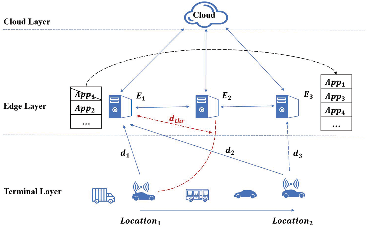
Figure 1: Schematic diagram of a container-based edge-cloud architecture and service migration scenarios

Through the above scenario description, the research content of this paper can be divided into the following three questions: (1) When will the migration action happen? i.e., to define the triggering conditions for the migration decision; (2) Where will the application be migrated? i.e., to judge the best target edge server; (3) How to carry out the migration process? i.e., to design the migration model and migration algorithm.

The organization of the rest paper is as follows: Section 2 describes the process of establishing a container application migration model based on edge computing in the IoV business scenario. Section 3 introduces the process of designing a container application migration algorithm based on dynamic programming. Section 4 shows the results of simulation experiments and compares the algorithm proposed in this paper with the other two algorithms. Section 5 summarizes the research work of this paper and discusses some subsequent problems to be solved.

2  Application Migration Model

This section introduces the process of establishing the migration model that used in this paper.

2.1 Problem Analysis

(1) When to migrate?

This part defines the trigger conditions for migration.

Define the pre-judgment radius as dpre ( dpre<dthr , where dthr is the coverage radius of the edge server service domain). When the distance from the connected vehicle to the center of the local service domain exceeds dpre , the vehicle tends to continue driving away from the local service domain, and the vehicle has no stopover halfway (i.e., the vehicle’s speed should be greater than or equal to V , usually set V=30km/h in urban road scenarios [12,13]), the connected vehicle has reached the migration trigger condition, then immediately preparing for migration.

(2) Where to migrate?

This part describes how to select the target server.

This paper mainly discusses two driving road scenes. One is a straight road scene without branch roads, as is shown in Fig. 2a; the other is a crossroad scene including T-shaped branch roads, as is shown in Fig. 2b.

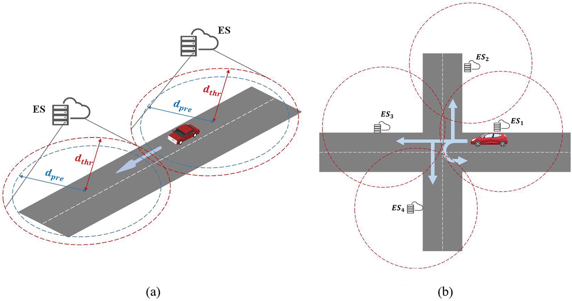
Figure 2: Two driving road scenes (a) straight road scene (b) crossroad scence

For the straight road scene, since the connected vehicle can only keep going ahead (as is shown in Fig. 2a), the target server is easily determined, which can be directly selected as the next available server along the road. For the crossroad scene, since there are four driving options for the vehicle at the intersection (as is shown in Fig. 2b): go straight, turn left, turn right, and turn around, thereby the target server is not easy to be chosen. It needs to combine the actual traffic conditions, navigation, and other perception information to make prediction judgments [14,15].

(3) How to migrate?

This part introduces three ideas to design the migration strategy [16,17].

In the migration scenario of single-vehicle and single-application, this paper focuses on the migration scenario of crossroads. For vehicles that are on the edge of crossroads and are about to undergo application migration, based on the acquired vehicle trajectory data, this paper considers three selection standards:

The first is the nearest selection method: select the available edge server closest to the connected vehicle at the current time as the target server.

The second is the local optimal method: select the available edge server with the least migration cost at the current time as the target server.

The third is the dynamic programming method: select the next-turn edge server corresponding to the migration path that minimizes the total migration cost in the future limited observation time as the target server.

This paper proposes the third one, the dynamic programming method. Based on the goal of minimizing the total migration cost, to design the migration model (in Section 2.2) and migration algorithm (in Section 3) and then compare the third method with the first and the second method (in Section 4).

2.2 Model Building

First, make some definitions. Set the time slot t=1,2,3,… , the length of each time slot is τ . The driving trajectory in the time slot t is L(t) . The maximum tolerable delay of the vehicle application m is Dmax . Considering the urban road scene, suppose that there are N edge servers in the edge network of a certain area. Define a matrix π with a dimension of Q×N , and use it to represent the application deployment in consecutive Q time slots, where the value of the matrix elements can only be 1 or 0. For example, the matrix element πt,n=1 means that the application is deployed on the edge server n in the time slot t . Otherwise, πt,n=0 means that the application is not deployed on this server. In this way, obtain the migration situation of the application by observing the changes in the values of the two adjacent elements of the matrix π , i.e., the matrix π represents the migration decision in consecutive Q time slots, and π(t,t+1) represents the migration decision of two consecutive times. Define some indicators and parameters as follows:

(1) Communication delay

(a) Transmission delay

Trans(t)=λm,nηL(t)+Dextra (1)

where λm,n represents the amount of data packets sent by the migrating application; ηL(t) represents the maximum data transfer rate between the connected source and target edge servers; Dextra represents additional costs such as queuing delay.

(b) Calculation delay

Comp(t)=φmλm,nεm,n+Dqueue (2)

where φm represents the calculation demand of the data packet sent by the application; εm,n represents the amount of bits that the target edge server can process for the application in each time slot; Dqueue represents the queuing delay.

In summary, define the communication delay as follows:

costcomm(t)=Trans(t)+Comp(t) (3)

(2) Migration delay

costmig(t)=θmηL(t)+Dfrozen (4)

where θm represents the amount of migration data generated by the application migrating from the source edge server to the target edge server; Dfrozen represents the freezing time of the container during the process of migrating the application.

(3) Target server status

In order to avoid service interruption, when performing the migration decision, consider the communication delay and the migration delay and also consider whether the target server can provide enough resource space for the migrating application.

Suppose that the application m needs to occupy bandwidth capacity bm and storage capacity cm . For the source server src and target server dst , represent the current idle bandwidth capacity respectively by Bsrc and Bdst , and represent the storage capacity represented by Csrc and Cdst . The changes in the process of migrating the application m from the source server to the target server are as follows:

Bsrc=Bsrc+bm (5)

Bdst=Bdst−bm (6)

Csrc=Csrc+cm (7)

Cdst=Cdst−cm (8)

(4) Direction of movement

In addition to the above factors, the moving trend of vehicles will also affect the migration decision. Suppose the vehicle moves from point A to point B in unit time t , and define the direction vector from point A to point B as the moving direction of the vehicle at time t , denoted as m→t , then express the moving direction of the vehicle at the previous time t−1 as m→t−1 . Use the projection of m→t on m→t−1 to measure their direction consistency, as follows:

|m→t|cos⁡Θ=m→t⋅m→t−1|m→t−1| (9)

where Θ is the angle between the moving directions of the vehicle at two adjacent times. When the projection value is positive ( |m→t|cos⁡Θ>0 ), the vehicle’s moving directions are considered to be basically the same, and positive feedback is given to the execution of the migration decision; when the projection value is not positive ( |m→t|cos⁡Θ≤0 ), it is considered that the moving directions of the vehicle are reversed, and negative feedback is given to the execution of the migration decision.

(5) Optimization problem

Define the cost function as:

C(t)=costcomm(t)+costmig(t) (10)

where C(t) represents the delay of single application migration, and let C(t)≤Dmax . Besides, the following prerequisites should be met:

Bdst−bm≥0 andCdst−cm≥0 and|m→t|cos⁡Θ>0 (11)

The above formulas show that the migration decision is meaningful only when the target server has sufficient resource space for the migrating application and the vehicle follows the direction of driving away from the local service domain.

This paper takes a limited time T to represent the long-term time. Then the long-term total cost is defined as:

C=∑t=t0t0+T−1C(t) (12)

Then the optimization problem can be expressed as:

π=arg⁡minπCs.t.C(t)≤Dmax,∀t (13)

This problem can be converted into the shortest path problem and use dynamic programming to solve it.

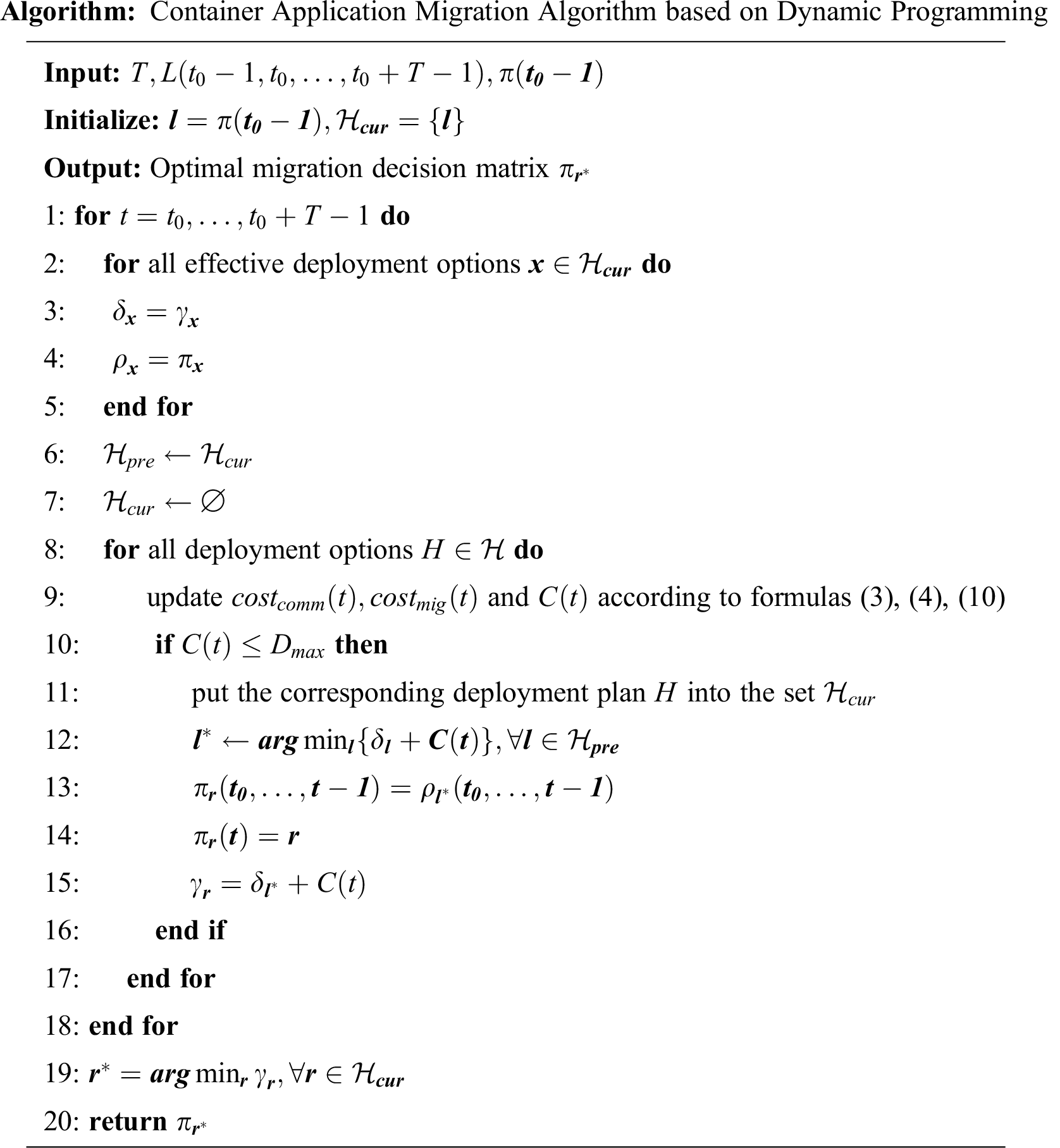
3  Dynamic Programming Migration Algorithm

This section introduces the design process of the migration algorithm based on dynamic programming. Define all possible deployment schemes of π(t) as set H , and then there are at most N elements in this set ( N is the number of edge servers). Define vectors r=π(t) and l=π(t−1) , r∈H and l∈H , to represent the application deployment situation at the current time and the previous time, respectively. Define sets Hcur⊆H and Hpre⊆H to record the effective deployment schemes which meet the constraints at the current time and the previous time, respectively. Define variable γx to represent the sum of C(t) from time t0 to the current time when the application deployment is x and the application deployment is optimal until the current time. Define variable δx to represent the sum of C(t) from time t0 to the previous time when the application deployment is x and the application deployment is optimal until the previous time. Define vectors πx and ρx to respectively cache the optimal migration strategy from time t0 to the current time and the previous time when the application is deployed as x . Suppose the initial position of the connected vehicle is L(t0−1) , the trajectory result of the vehicle in the next T time is L(t0,…,t0+T−1) , and the initial application deployment is π(t0−1) . The process of application migration algorithm using dynamic programming to select the optimal strategy is as follows:

When the initial state π(t0−1) is determined, for all effective deployment schemes x∈Hcur at the current time slot t0 , to establish a state transition relationship for subsequent iterative multiplexing. According to the constraints, put the deployment solutions that meet the conditions in the set Hcur . For each deployment situation in the set Hcur , obtain the optimal migration solution from the previous time slot to the current time slot by solving the Bellman equation, cache the optimal migration strategy (i.e., the deployment matrix) up to the last time slot and calculate the sum of C(t) up to the last time slot for subsequent multiplexing. Through T iterations, seek the deployment solution r∗ that minimizes the total cost C (i.e., the sum of C(t) ), and return to its corresponding migration decision matrix πr∗ , then locating the current time slot to obtain the best migration decision.

4  Experiments

This section introduces the results of the simulation experiments, then analyzes the results compared with the other two algorithms.

This experiment was conducted using MATLAB simulation software to compare the container application migration algorithm based on dynamic programming proposed in this paper (hereinafter referred to as DPMA) with the container application migration algorithm based on the standard of selecting the nearest available target server (hereinafter referred to as NRMA) and the container application migration algorithm based on the standard of choosing the target server that minimizes the current migration cost (hereinafter referred to as LOMA), respectively. In the simulation experiment, set the same map, the same distribution of edge servers, and the same vehicle trajectory for the three algorithms, then compare and analyze the results from the following aspects: total migration times, total migration cost, long-term average total cost and average single migration cost.

4.1 Parameter Value

The values of the model parameters used in this experiment are shown in Tab. 1.

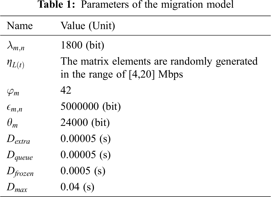
This experiment randomly generated 20 sets of data to form the data transmission rate matrix ηL(t) in the range of [4,20] Mbps, and thus 20 sets of simulation experiments were carried out. The problem of finding the optimal migration decision based on dynamic programming is equal to the shortest path problem. The graphshortestpath function in MATLAB can be used to visually display the migration path, as is shown in Fig. 3 (only show the first group of simulation results as an example).

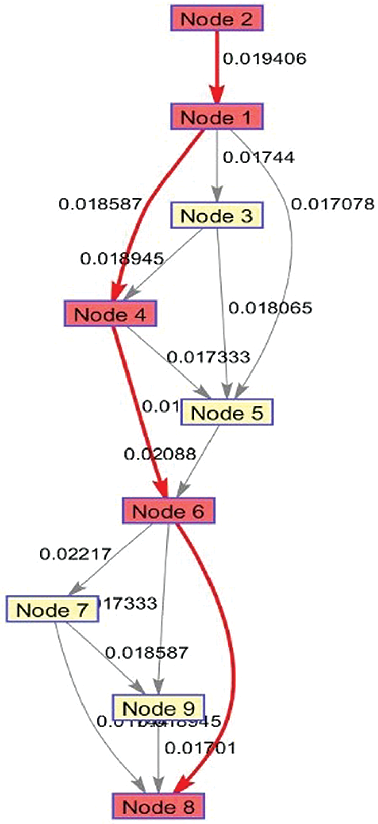
Figure 3: Shortest path visualization

In Fig. 3, the node number corresponds to the number of the edge server, the weight between the two nodes represents the migration cost from the previous node (i.e., source server) to the next node (i.e., target server), and the red line indicates the shortest path from the start point to the endpoint, which is the global optimal solution for the migration decision, and then track the path can get the best migration choice at every moment.

4.2 Results Analysis

(1) Total migration times

As is shown in Fig. 4, in this experiment, the total migration times of DPMA remain at 4, the total migration times of NRMA remain at 6, and the total migration times of LOMA fluctuate between 4 and 7. Since the application migration process will inevitably consume resources and might cause network faults or service interruptions, theoretically, in order to reduce latency, save consumption, and improve network stability, so make the migration times as few as possible.

(2) Total migration cost and long-term average total cost

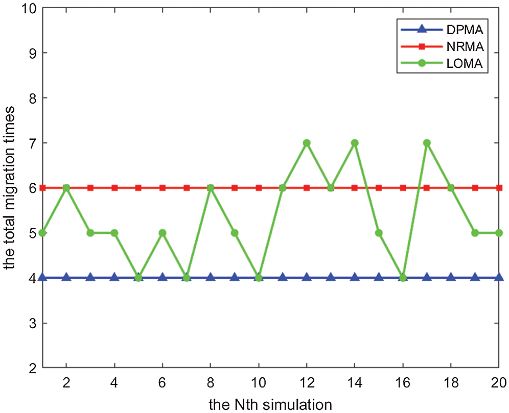
Figure 4: Total migration times

As is shown in Fig. 5, the total migration cost generated by DPMA and NRMA does not fluctuate much, while the total migration cost of LOMA fluctuates greatly. In addition, the long-term average total cost of the three algorithms is shown by dashed lines in Fig. 5. The comparison shows that the long-term average total cost of DPMA is 33.88% and 24.53% lower than NRMA and LOMA, respectively.

(3) Average single migration cost

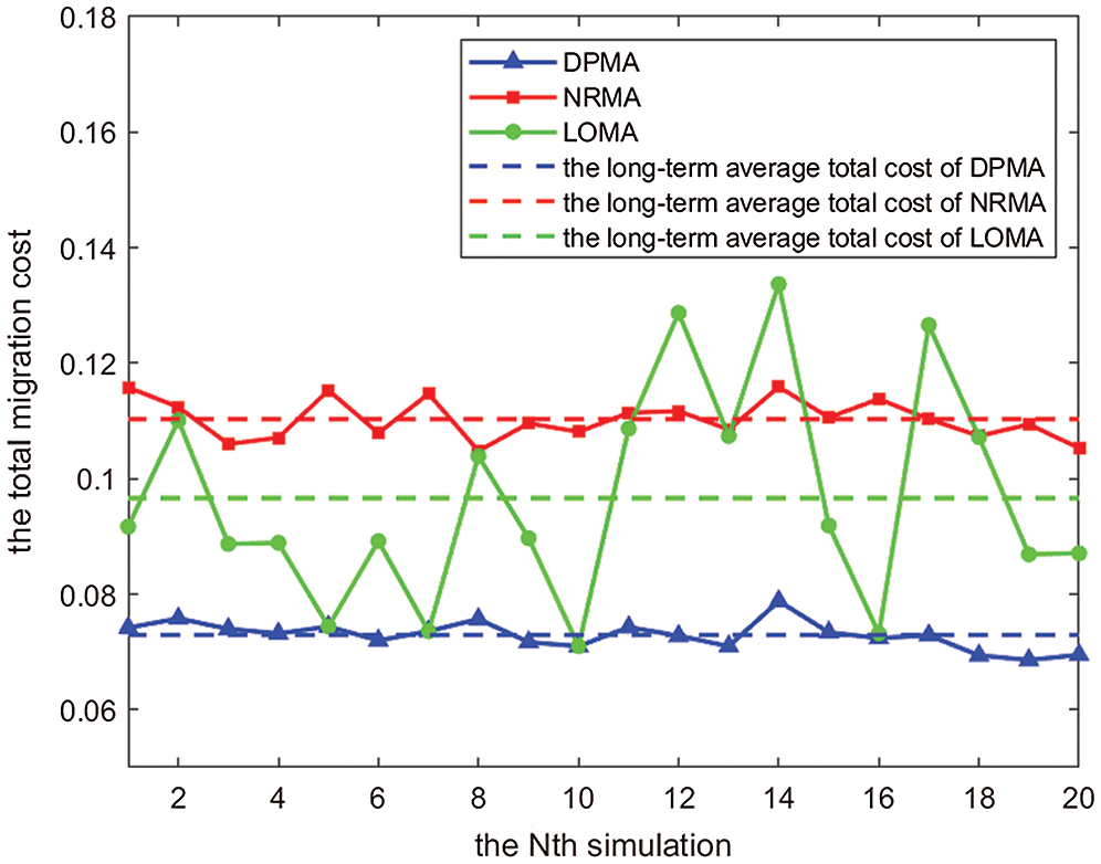
Figure 5: Total migration cost and long-term average total cost

The standard of LOMA is to select the target server with the least migration cost at the current migrating moment, so in most cases, its value of the cost that averages to a single migration is the smallest (as is shown in Fig. 6).

Figure 6: Average single migration cost

However, LOMA is easy to fall into the local optimal deadlock (as is shown in Fig. 7). That is, the local optimal migration choice at the current moment may cause negative impacts on the migration choice at the later moment and eventually consume more migration costs.

Figure 7: The local optimal deadlock (green line represents LOMA) (a) Group 16th (b) Group 17th

4.3 Experiments Summary

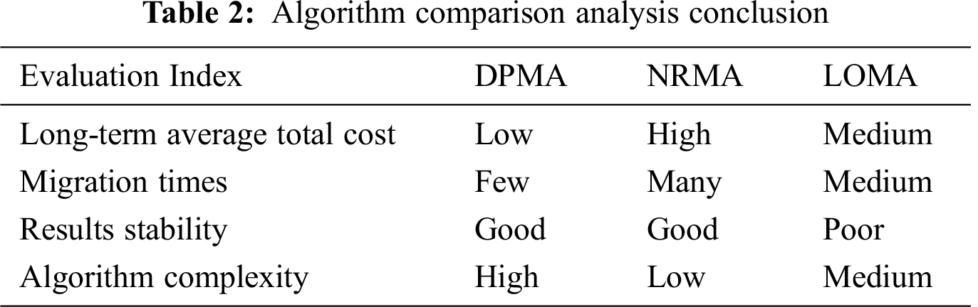
In summary, the container application migration algorithm based on dynamic programming can ensure the minimal total migration cost and the minimal total migration times, as well as, it can adapt to different network channel capacity conditions. Therefore, it is suitable for single vehicle and single application migration scenarios. The comparative analysis of DPMA, NRMA and LOMA is shown in Tab. 2:

5  Conclusions

This paper builds a container application migration model based on edge computing in the IoV business scenario, uses time delay to measure the migration cost, divides the migration cost into communication delay and migration delay, and considers the target server status and vehicle movement trends to judge whether to perform the migration decision. Then, this paper designs an application migration algorithm based on dynamic programming and uses the shortest path principle to obtain the global optimal solution of the migration decision. Finally, the simulation experiments show that the long-term average migration cost of the dynamic programming migration method proposed in this paper is significantly lower than the other two migration algorithms used for comparison, i.e., the dynamic programming migration method performs better.

The future research work would consider the migration scenarios of multiple vehicles and multiple applications.

Acknowledgement: The work is supported by the Science and Technology Project of State Grid Zhejiang Electric Power Co., Ltd (5211XT19006F).

Funding Statement: The authors received no specific funding for this study.

Conflicts of Interest: The authors declare that they have no conflicts of interest to report regarding the present study.

References

 1.  W. S. Shi, J. Cao, Q. Zhang, Y. H. Z. Li and L. Y. Xu, “Edge computing: Vision and challenges,” IEEE Internet of Things Journal, vol. 3, no. 5, pp. 637–646, 2016. [Google Scholar]

 2.  A. Alhussain, H. Kurdi and L. Altoaimy, “A neural network-based trust management system for edge devices in peer-to-peer networks,” Computers, Materials & Continua, vol. 59, no. 3, pp. 805–816, 2019. [Google Scholar]

 3.  T. F. Yang, X. J. Shi, Y. Y. Li, B. B. Huang, H. Y. Xie et al., “Workload allocation based on user mobility in mobile edge computing,” Journal on Big Data, vol. 2, no. 3, pp. 105–115, 2020. [Google Scholar]

 4.  Z. Q. Tang, X. J. Zhou, F. M. Zhang, W. J. Jia and W. Zhao, “Migration modeling and learning algorithms for containers in fog computing,” IEEE Transactions on Services Computing, vol. 12, no. 5, pp. 712–725, 2019. [Google Scholar]

 5.  S. G. Wang, J. L. Xu, N. Zhang and Y. J. Liu, “A survey on service migration in mobile edge computing,” IEEE Access, vol. 6, pp. 23511–23528, 2018. [Google Scholar]

 6.  O. Salman, I. Elhajj, A. Kayssi and A. Chehab, “Edge computing enabling the Internet of Things,” in IEEE 2nd World Forum on Internet of Things (WF-IoT 2015). Milan, Italy, pp. 603–608,2015. [Google Scholar]

 7.  B. I. Ismail, E. M. Goortani, M. B. A. Karim, W. M. Tat, S. Setapa et al., “Evaluation of docker as edge computing platform,” in IEEE Conf. on Open Systems (ICOS 2015Melaka, Malaysia, pp. 130–135, 2015. [Google Scholar]

 8.  N. Yuan, C. Jia, J. Lu, S. Guo, W. Li et al., “A DRL-based container placement scheme with auxiliary tasks,” Computers, Materials & Continua, vol. 64, no. 3, pp. 1657–1671, 2020. [Google Scholar]

 9.  A. E. Elgazar and K. A. Harras, “Enabling seamless container migration in edge platforms,” in CHANTS’19: Proc. of the 14th Workshop on Challenged Networks, New York, NY, USA, pp. 1–6, 2019. [Google Scholar]

10. U. Bjorkengren, “Technologies for application migration using lightweight virtualization,” U.S. Patent, no. 9971622, 2018. [Google Scholar]

11. C. Pahl and B. Lee, “Containers and clusters for edge cloud architectures--a technology review,” in 3rd Int. Conf. on Future Internet of Things and Cloud (FiCloud 2015Rome, Italy, pp. 379–386, 2015. [Google Scholar]

12. X. Yu, M. L. Guan, M. X. Liao and X. Fan, “Pre-migration of vehicle to network services based on priority in mobile edge computing,” IEEE Access, vol. 7, pp. 3722–3730, 2019. [Google Scholar]

13. M. L. Guan, “Research on the pre-migration strategy of MEC Internet of Vehicles application,” Chongqing: M.S. theses, Chongqing University of Posts and Telecommunications, 2019. [Google Scholar]

14. J. Liu, X. Kang, C. Dong and F. Zhang, “Simulation of real-time path planning for large-scale transportation network using parallel computation,” Intelligent Automation & Soft Computing, vol. 25, no. 1, pp. 65–77, 2019. [Google Scholar]

15. H. Gao, W. Huang and X. Yang, “Applying probabilistic model checking to path planning in an intelligent transportation system using mobility trajectories and their statistical data,” Intelligent Automation & Soft Computing, vol. 25, no. 3, pp. 547–559, 2019. [Google Scholar]

16. P. Li, H. Q. Nie, H. Xu and L. Dong, “A minimum-aware container live migration algorithm in the cloud environment,” International Journal of Business Data Communications and Networking, vol. 13, no. 2, pp. 15–27, 2017. [Google Scholar]

17. J. Y. Chen, “Design and implementation of service migration strategy in mobile edge computing environment,” Beijing: M. S. theses, Beijing University of Posts and Telecommunications, 2018. [Google Scholar]

This work is licensed under a Creative Commons Attribution 4.0 International License, which permits unrestricted use, distribution, and reproduction in any medium, provided the original work is properly cited.