DOI:10.32604/iasc.2021.018496
| Intelligent Automation & Soft Computing DOI:10.32604/iasc.2021.018496 | |
| Article |
Inversion of Temperature and Humidity Profile of Microwave Radiometer Based on BP Network
1School of Artificial Intelligence, Nanjing University of Information Science and Technology, Nan Jing, 210044, China
2School of Computer and Software, Nanjing University of Information Science and Technology, Nan Jing, 210044, China
3International Business Machines Corporation (IBM), NY, 100014, USA
*Corresponding Author: Yong Jun Ren. Email: renyj100@126.com
Received: 10 March 2021; Accepted: 14 April 2021
Abstract: In this paper, the inversion method of atmospheric temperature and humidity profiles via ground-based microwave radiometer is studied. Using the three-layer BP neural network inversion algorithm, four BP neural network models (temperature and humidity models with and without cloud information) are established using L-band radiosonde data obtained from the Atmospheric Exploration base of the China Meteorological Administration from July 2018 to June 2019. Microwave radiometer level 1 data and cloud radar data from July to September 2019 are used to evaluate the model. The four models are compared with the measured sounding data, and the inversion accuracy and the influence of cloud information on the inversion are subsequently analyzed. The results show the following: the average errors of temperature and humidity profiles for the model without cloud information are 1.18°C and 11.7%, while the average errors of temperature and humidity profiles for the model with cloud information are 0.71°C and 6.09%. Compared with the profiles that lack cloud information, the RMSE of most altitudes is reduced to some extent after cloud information is added, which is particularly obvious at layers where cloud is present.
Keywords: Ground-based microwave radiometer; BP neural network; atmospheric temperature and humidity profiles; cloud information
Temperature and humidity are very important indicators in the field of climate research, as they can directly reflect the heat and water vapor conditions in the atmosphere and have a clear impact on the accuracy of meteorological products. Grasping real-time changes in the temperature and humidity profile is of great significance for satellite positioning, warning, artificial weather modification and other such meteorological activities. It is thus particularly important to accurately detect atmospheric indicators in real time in order to obtain temperature and humidity profile information. Previously, traditional weather detection methods have primarily used sounding balloons, sounding rockets, satellite remote sensing methods and other technical means to measure elements in the atmosphere and obtain the temperature and humidity profiles over time. In 1985, Liu [1] began to use VHF radar to detect the observational data of the atmospheric structure and inverted the temperature profile; in 1990, Wang [2] used the improved empirical orthogonal function (EOF) expansion method and the simulated radiant temperature values of six O25mm channels in the satellite Advanced Microwave Sounder (AMSU) to perform experiments that inverted the vertical distribution of atmospheric temperature, with good results; moreover, in 2003, Wu et al. [3] investigated satellite detection techniques for both infrared hyperspectral and inversion methods using existing airborne and satellite-borne hyperspectral data, focusing on the inversion method of the atmospheric infrared detector AIRS, and summarized the process of a standardized inversion method; in 2010, Dong et al. [4] analyzed the main features of the Fengyun-3A (FY-3A) meteorological satellite and identified the various applications that can be made to its observational data processing to generate the distribution of changes in atmospheric temperature and humidity, and provided new ideas; in 2017, Zhou [5] compared and analyzed the models of temperature and humidity profiles inverted by FY-4 hyperspectral infrared vertical detector (GIIRS) and Metop-A hyperspectral infrared vertical detector (Iasi). The analysis results show that the inversion accuracy of atmospheric temperature by GIIRS is inferior to that of Iasi in the upper layer, Other aspects are superior to Iasi; in 2019, Guan et al. [6] studied the variational inversion method of the atmospheric temperature and water vapor mixing ratio profile based on Metop-A/Iasi infrared hyperspectral data. The experimental results show that the atmospheric temperature and water vapor mixing ratio profile can be detected with high precision through the use of Metop-A/Iasi infrared hyperspectral data based on the one-dimensional variational method. However, the characteristically low spatial and temporal resolution of sounding balloons cannot meet the development requirements of modern meteorology, while remote sensing satellites will suffer due to cloud cover and poor detection effect at low-altitude latitudes. Therefore, many experts and scholars have committed themselves to the study of ground-based remote sensing technology for atmospheric detection. Among these techniques, microwave radiometer equipment based on ground-based remote sensing technology is relatively mature. Microwave radiometers have been widely used in atmospheric temperature and humidity profile detection, and are also complementary with other sounding equipment data; this has produced good results, including cloud radar, etc. However, the principle behind microwave radiometers is to obtain the brightness temperature of the atmosphere in order to invert the temperature and humidity profile by receiving the atmospheric thermal radiation. However, this detection principle also means that the equipment has certain limitations. It has been found that different regions, seasons, climates, quality control algorithms and inversion algorithm models will have differing impacts on the inversion effect of the microwave radiometer; among these, cloud weather factors have the most significant impact on the inversion effect of the microwave radiometer. Based on the above analysis, this paper will apply the cloud information measured via millimeter wave cloud radar to the inversion process, build two sets of inversion algorithm models on the basis of the BP neural network algorithm, distinguish between the two depending on whether or not cloud information is added, and use sounding data as the standard. By comparing the prediction results of the two models with the actual situation, the influence of the cloud cover information on the inversion of the atmospheric temperature and humidity profile can be analyzed. The remainder of this paper is structured as follows. The second part primarily introduces the related work conducted by predecessors in this field. The third section introduces the data and algorithms used in this paper. The fourth section compares and analyzes the experimental results. Finally, the fifth section summarizes the experiments and improved results presented in this paper.
Microwave radiometer is not a very new type of equipment; as early as the 1960s, related scholars began research into and accuracy correction of microwave radiometers. In 1969, Westwater et al. [7] began to explore ground-based microwave remote sensing, successfully developed microwave radiometers for k-wave end (water vapor microwave absorption peak area) and V-band (oxygen microwave absorption peak area), and inverted the atmospheric temperature profile. In 1985, Chedin et al. [8] explored the atmospheric transmission process, proposed the pattern recognition method, selected the approximate optimal solution from multiple groups of data, and then used the Bayes algorithm to invert the temperature and humidity profile. In 1986, Wang et al. [9] used a microwave radiometer to detect the atmospheric temperature and thereby improved the inversion accuracy of the temperature profile. In 2011, Liu et al. [10] analyzed the accuracy of the temperature profile data measured via ground-based microwave radiometer an observatory in southern suburban Beijing. In 2012, Wang et al. [11] set up training samples to train neural network models for different types of weather and different seasons. Their results showed that the neural network model’s calculation accuracy is significantly better than the network algorithm built into the ground-based microwave radiometer. In 2013, Sanchez et al. [12] proposed a plan for quality control along the height of the MP-3000A ground-based microwave radiometer in order to obtain a more accurate atmospheric profile. In 2014, Tan et al. [13] used an airborne microwave radiometer to analyze the influence of different combinations of channels, observation error, platform flight altitude and other factors on inversion performance. In 2015, Li et al. [14] compared and analyzed the secondary data of a microwave radiometer with the historical sounding data, corrected the deviation of the data and obtained a result that is closer to the sounding data. In 2018, Mao et al. [15] directly compared and analyzed the first-level brightness temperature data observed by the microwave radiometer, investigating the detection accuracy of the microwave radiometer in different types of weather and different seasons. In 2019, Wu et al. [16] compared the accuracy errors of specific radiometers horizontally and further analyzed the internal and external errors of inversion errors for a mp3000a microwave radiometer. In 2020, Xu et al. [17] compared the accuracy errors of certain radiometers with those of small UAVs. The temperature and humidity data inverted from the simultaneous observations of the radiosonde and microwave radiometer further prove the microwave radiometer’s performance; it appears that the detection and inversion ability is improved through the application of this method. Since the inception of the microwave radiometer, numerous experts and scholars have applied it to the inversion of temperature and humidity profiles, and have carried out research into the algorithm to improve the inversion performance. Common methods include the Kalman filter method, optimal estimation method, Newton iteration method, statistical regression method, empirical orthogonal function method, control least square method, best extension method, estimation theory methods, artificial kernel function method, Monte Carlo method, neural network method, etc. [18]. The optimal estimation method has several advantages including algorithmic simplicity, high accuracy, and ability to show abnormal changes. However, it depends on historical data, which requires a large amount of calculation and is thus incapable of meeting the real-time requirements for obtaining temperature and humidity profiles. The Monte Carlo method does not rely on historical data, but still encounters the same fatal problem as the optimal estimation method (i.e., a long operation time). For its part, the Kalman filter method has strong adaptability, is suitable for real-time processing, and can provide an estimation error variance while making an estimate; however, an accurate filtering model needs to be established, and the problem of filtering divergence still remains. The statistical regression algorithm has high accuracy and fast speed, can detect abnormal changes, and is stable overall; however, the model needs to be established in advance. The neural network algorithm has the same advantages as statistical regression, but also has the “black box” effect; therefore, it does not require building a model in advance. Finally, it achieved narrow victory in the competition between algorithms, and is thus widely used in the microwave radiometer inversion process. In 2011, Yang et al. [19] used a neural network algorithm to invert the temperature and humidity profile on sunny days, proving the extraordinary nonlinear fitting ability of the neural network algorithm, which can be used to invert the temperature and humidity profile. In 2013, Huang et al. [20] used the neural network and multiple linear regression algorithms to invert the temperature and humidity profile under the same experimental sample conditions, obtaining results showing that the neural network algorithm achieves a better inversion effect. In 2018, after conducting quality control and correction of the original brightness temperature data observed by the microwave radiometer, Bao et al. [21] utilized the neural network algorithm to invert the atmospheric temperature and humidity profile, obtaining good results.
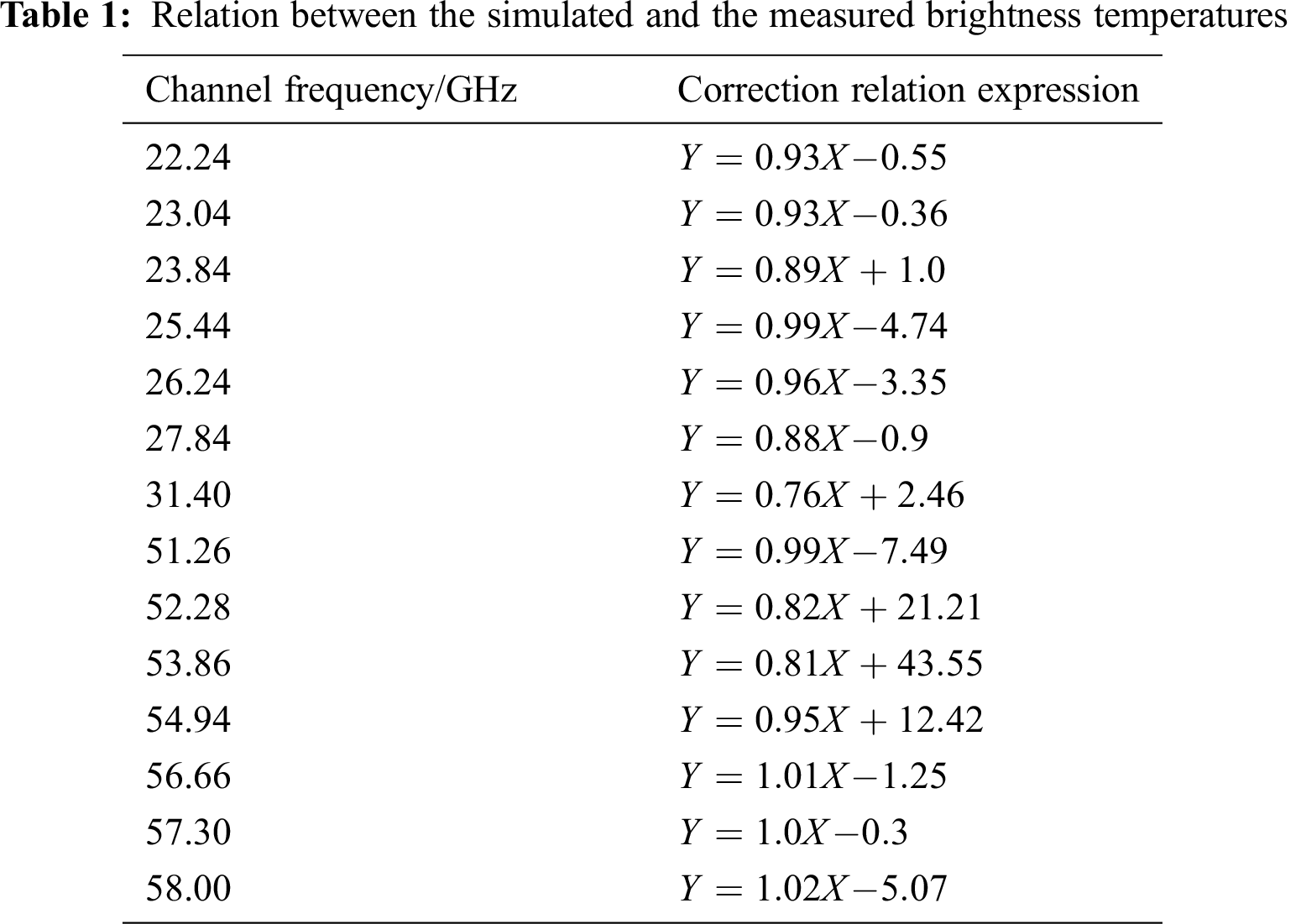
The data used in this paper are primarily sounding data, microwave radiometer data and millimeter-wave cloud radar data. Among these, the sounding data is L-band sounding data obtained twice per day in the meteorological station in a southern suburb of Beijing, China from July 2018 to June 2019. The microwave radiometer data is obtained from the Airda-HTG3 14 channel microwave radiometer installed at the Atmospheric Exploration and Test base of the China Meteorological Bureau. Among them, the K-band (22~32 GHz) and V-band (51~59 GHz) each have seven channels, the center frequencies of which are 22.24, 23.04, 23.84, 25.44, 26.24, 27.84, 31.4, 51.26, 52.28, 53.86, 54.94, 56.66, 57.3 and 58 GHz. While there are four kinds of data output, we only need to select Level 1 (first-level quality control) data to obtain the brightness temperature data. The data range is from January 2019 to September 2019; the millimeter-wave cloud radar data is from July 2019. As of September 2019, the Ka-band 35 GHz all-solid-state vertical-pointing Doppler weather radar of the Beijing Meteorological Station has a measuring height of 12 km, a vertical spatial resolution of 30 m, and an adjustable time resolution of 1~60 s.
In theory, the neural network algorithm can approach any complex nonlinear relationship, and it is not necessary to design a highly complex inversion algorithm. It has thus been successfully used in the field of atmospheric parameter profile inversion and is a relatively mature and widely used inversion algorithm. In this paper, four sets of inversion models are proposed: model A1 and model A2, with no cloud information added in the input layer, and model B1 and model B2, with six cloud information nodes added in the input layer on the basis of model A. The four sets of models all use a three-layer feedforward BP neural network. The hyperbolic tangent sigmoid transfer function tansig is selected from the input layer to the hidden layer, while the linear transfer function purelin is selected from the hidden layer to the output layer, enabling continuous function mapping to be realized with arbitrary precision. There are 17 nodes in the Model A input layer (without cloud information). The first 14 nodes are the measured brightness temperature values of 14 channels of the microwave radiometer, while the last three nodes are the ground temperature, relative humidity and pressure. The number of output layer nodes is set to 83: that is, the temperature or relative humidity at the 83 height layers, divided from the ground to the height of 10 km. The specific layering method is as follows: 0–500 meters every 25 meters, 500–2000 meters every time there is a floor of 50 meters, and a floor of 250 meters every 2000–10000 meters. Due to the high-speed requirement for atmospheric profile inversion in practical applications and the singular nature of the data samples used in this paper, a single hidden-layer structure is utilized. The number of hidden layer nodes is calculated according to the formula proposed in Gao [22].
In Eq. (1),
Building a BP neural network model for inverting temperature and humidity profiles requires a large amount of microwave radiometer data to be available for use as samples. However, due to the limited amount of measured microwave radiometer data and cloud radar data, this paper opts to use L-band sounding data as sample data. The first fourteen nodes of the input data for model training are the brightness temperature values, which are not included in the radiosonde data. This paper utilizes the radiation transmission mode to simulate the brightness temperature data of the microwave radiometer that corresponds to the sounding data. First, the radiosonde data is taken as the input data, while the MonoRTM radiation transmission mode is used to simulate and calculate the Level 1 brightness temperature data of the microwave radiometer. The final three nodes of the input data are the surface temperature, humidity and pressure values; in the sounding data, these are the temperature, humidity and pressure values corresponding to the bottom height. In Model B (with cloud information added), the input node has six additional cloud layer data points. We determine whether the relative humidity of each height layer reaches 85% in order to gauge whether it is entering or exiting the cloud, then calculate the sample corresponding to the three layers of bottom cloud height and cloud thickness as the sample input of the last six nodes. [23,24]. The output data of the model training is the temperature and humidity values that correspond to the 83 altitude layers. The appropriate temperature and humidity values can be obtained by interpolating the sounding data. The samples utilized in the model training contain sounding data obtained at China Meteorological Administration’s atmospheric sounding test base from July 2018 to June 2019, with a total of 700 valid data points. During the training process, 70% of the samples are used as the training set, with the remaining 30% used as the test set. The model quality is evaluated by means of cross-validation.
3.4 Brightness Temperature Correction
The brightness temperature is the actual measured value of the microwave radiometer. The accuracy of the brightness temperature data directly affects the accuracy of the inversion result. Due to the differences between the microwave radiometer equipment and the detection effect, a difference still remains between the measured brightness temperature and the simulated brightness temperature [25]. This experiment uses sounding data to simulate the brightness temperature during the model training process, while the actual measured brightness temperature is used during the inversion. The difference between the two causes bias in the inversion results. Therefore, the actual brightness temperature measured by the microwave radiometer is used to invert the temperature and humidity profile. Before line is inverted, it is necessary to correct the deviation of the brightness temperature value. Using the measured and simulated brightness temperature from January to June 2019, the linear fitting of the measured and simulated brightness temperatures is performed on each channel. Finally, the corrected relationship expression of the measured brightness temperature is obtained as shown in Tab. 1; here,
In this experiment, sounding data from July 2018 to June 2019 are used to train the model. For the model without cloud information, the simulated brightness temperature, ground temperature and humidity pressure data are used as input, while the corresponding observation time sounding temperature and humidity profile are used as the output to train the neural network. Moreover, for the model with cloud information, six nodes (the cloud base height and cloud thickness of three clouds) are added to the input node of the former, after which the model is trained in the same way.
3.6 Limitations of the Algorithm
The accuracy of the BP neural network inversion model studied in this paper can be easily affected by the quality of the training samples; a good model can only be trained using good-quality, representative training samples. However, due to the existence of instrumentation errors in the sounding balloon and the impact of wind on the observations, the temperature and humidity profile observed by the sounding instrument and the microwave radiometer detection of the temperature and humidity profile’s spatial location do not correspond; this will produce inversion errors, which represents a limitation of the inversion algorithm in this paper.
4 Experimental Results and Analysis
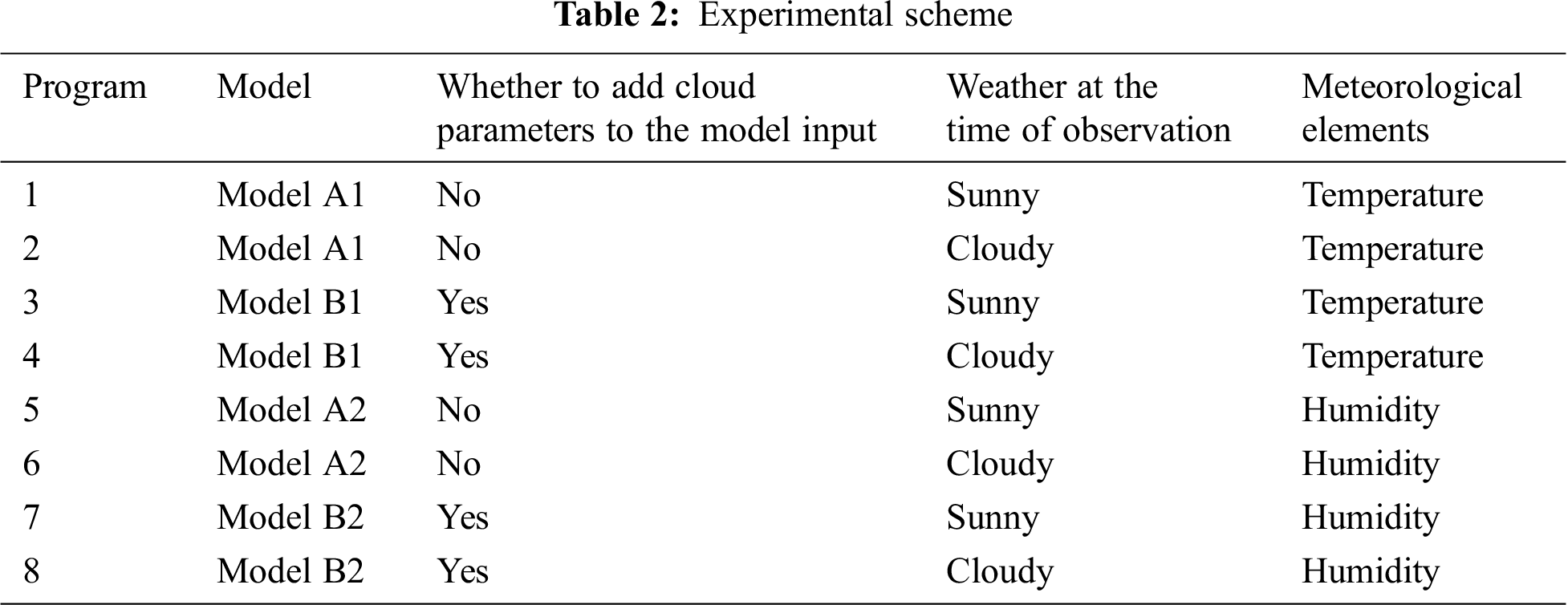
In this paper, we train four inversion models (model A1, model A2, model B1, model B2) according to whether or not cloud parameters are among the input factors. Depending on whether there are clouds (sunny days or cloudy days) within the range of 0–10 km, the test data are divided into eight experimental schemes. The two inversion models adopt different schemes to create a contrast comparison, then verify the actual effects of the two inversion models. These details are presented in Tab. 2.
Root mean square error is a statistic that describes the degree of data dispersion. The root mean square error (RMSE) is calculated as follows:
where,
The experiment in this paper uses sounding data as the standard, employing case analysis and statistical analysis to compare the inversion results of the two models with the sounding data. First, temperature and humidity profiles are drawn through the prediction of specific cases in order to visually demonstrate the model’s predictive ability; subsequently, we perform statistical analysis on the prediction results of the test samples, then calculate the RMSE value on each level to obtain a scientific prediction score curve.
4.3.1 Verification of Accuracy of Temperature Inversion Results
Fig. 1 presents the temperature profiles of the actual sounding data at 7:15 (UTC + 8) on September 8, 2019, along with the temperature profiles of model A1 and model B1 inversion obtained from the microwave radiometer LV1 product at that time. The weather at this observation time was sunny. As can be seen from the figure, the temperature profile inverted by the two models is essentially the same as the overall trend of the sounding data temperature profile. However, the model B1 curve with cloud information more closely resembles the actual curve; particularly at the heights of 4–5 km and 8–10 km, the predicted value of model A1 is relatively high, while the prediction result of model B1 can better reflect the actual vertical distribution of the atmospheric temperature. Fig. 2 presents the actual sounding data temperature profile at 13:15 (UTC+8) on July 21, 2019, along with the temperature profile comparison of Models A1 and B1 after the inversion of the microwave radiometer LV1 product at that time. The weather at observation time was cloudy. As can be seen from the graph, owing to the cloudy weather, the inverse effect of the temperature profile was affected to some extent. The temperature profiles inverted by the two models were both inferior to the inversion effect on sunny days in Fig. 1; at 0–6 km height, the prediction results of these two models are similar. At the height of 6–10 km, however, model B1 can still maintain a more accurate prediction result, while model A1 obviously deviates from the actual result. The error between model A1 and the actual curve thus increases rapidly, with the difference being largest at 10 km, reaching 11°C.

Figure 1: Comparison of atmospheric temperature profiles in sunny weather

Figure 2: Comparison of atmospheric temperature profiles under cloudy weather
Fig. 3 presents the root mean square error (RMSE) plots for the sunny day samples from July 1, 2019 to September 10, 2019. Here, temperature values from the actual sounding data are used as the standard to calculate the RMSE of the temperature results from the Model A1 and Model B1 inversions compared to the actual values at each altitude level. As can be seen from the figure, the prediction effects of both models can reach a good level. The average RMSE of model A1 is 0.62°C, while that of model B1 is 0.45°C. In terms of altitude level, the prediction results of the two models are similar at the 0–2 km altitude; at this altitude, the mean value of the RMSE difference between the two is only 0.08°C, while at altitudes above 2 km, the RMSE of Model A1 is significantly higher than that of Model B1. The average error of the former reaches 0.82°C, which is higher than that of the latter (0.52°C). As the height increases, the difference between the RMSE of the two undergoes a gradual increase, and the maximum difference reaches 0.84°C. This phenomenon is essentially consistent with the case in Fig. 1. It can be seen that, at low altitude, the prediction gap between the two models is not large. As the altitude increases, moreover, the prediction effect of model B1 with cloud information is still stable, which is significantly improved relative to model A1 without cloud information. Fig. 4 presents the root mean square error (RMSE) of cloudy samples from July 1, 2019 to September 10, 2019. Based on the temperature value of the actual sounding data, the root mean square error (RMSE) of the temperature results inverted by models A1 and B1 with the actual value calculated at each altitude level. As can be seen from the figure, compared with the sunny samples in Fig. 3, the error increases significantly when the weather is cloudy. The average RMSE of model A1 reaches 1.74°C, while the average RMSE of model B1 reaches 0.97°C, which is generally higher than is the case for sunny weather. This is because the appearance of clouds affects the observed brightness temperature of the microwave radiometer; this means that the inversion effect of cloud sky time will exhibit a greater deviation, which is consistent with the case in Fig. 2. It can further be seen that, under cloudy weather conditions, the inversion of temperature profiles becomes more difficult, with the prediction results of model A1 (without cloud information) deviating greatly from the actual values; by contrast, the model B1 (with added cloud information) is relatively stable and achieves obvious improvements. The addition of cloud information can thus effectively improve the inversion accuracy of the microwave radiometer’s atmospheric temperature profile under cloud conditions.

Figure 3: MSE comparison of atmospheric temperature profile inversion results in sunny weather
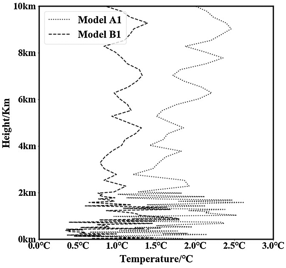
Figure 4: SE comparison of atmospheric temperature profile inversion results under cloudy weather
4.3.2 Accuracy Verification of Humidity Inversion Results
Fig. 5 presents the actual sounding data humidity profile at 13:15 (UTC+8) on August 29, 2019, along with the humidity profile comparison of Models A2 and B2 after inversion from the microwave radiometer LV1 at that time. At this observation time, the weather was sunny. As can be seen from the figure, the overall trend of the two humidity profiles inverted by the model in the low-altitude segment of 0–4 km is relatively close to the humidity profile of the sounding data. However, the inversion curve of Model B2 with added cloud information is closer to the actual curve, Moreover, in the high-altitude part above 5 km, the predicted value of Model A2 is generally lower by a factor of nearly 10%, while the maximum error is 20%. Compared with Model A2, the curve of B2 is significantly improved, more accurate, and yields prediction results that can better reflect the actual vertical distribution of atmospheric humidity. Fig. 6 presents the humidity profile of the actual sounding data at 07:15 (UTC + 8) on July 20, 2019, along with the humidity profile inverted by models A2 and B2 from the microwave radiometer LV1 product at that time. Weather conditions at this observation time were cloudy. The existence of the cloud layer has a substantial influence on the model’s inversion prediction effect. At this time, there are clouds at 0.2–1.9 km and 9.4–10 km. It can be seen from the figure that a significant difference exists between the prediction results of model A2 and the actual value in the cloud layer, while the model B2 (with cloud information) achieves obvious improvements, and its prediction results are similar to the actual value. At other cloud-free heights, the prediction results of the two models are similar to those of the sunny weather in Fig. 5, while the inversion curves of models A2 and B2 are close to the actual sounding curve.4.3.2 Accuracy verification of humidity inversion results.
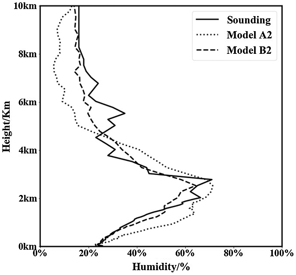
Figure 5: Comparison of atmospheric humidity profiles in sunny weather
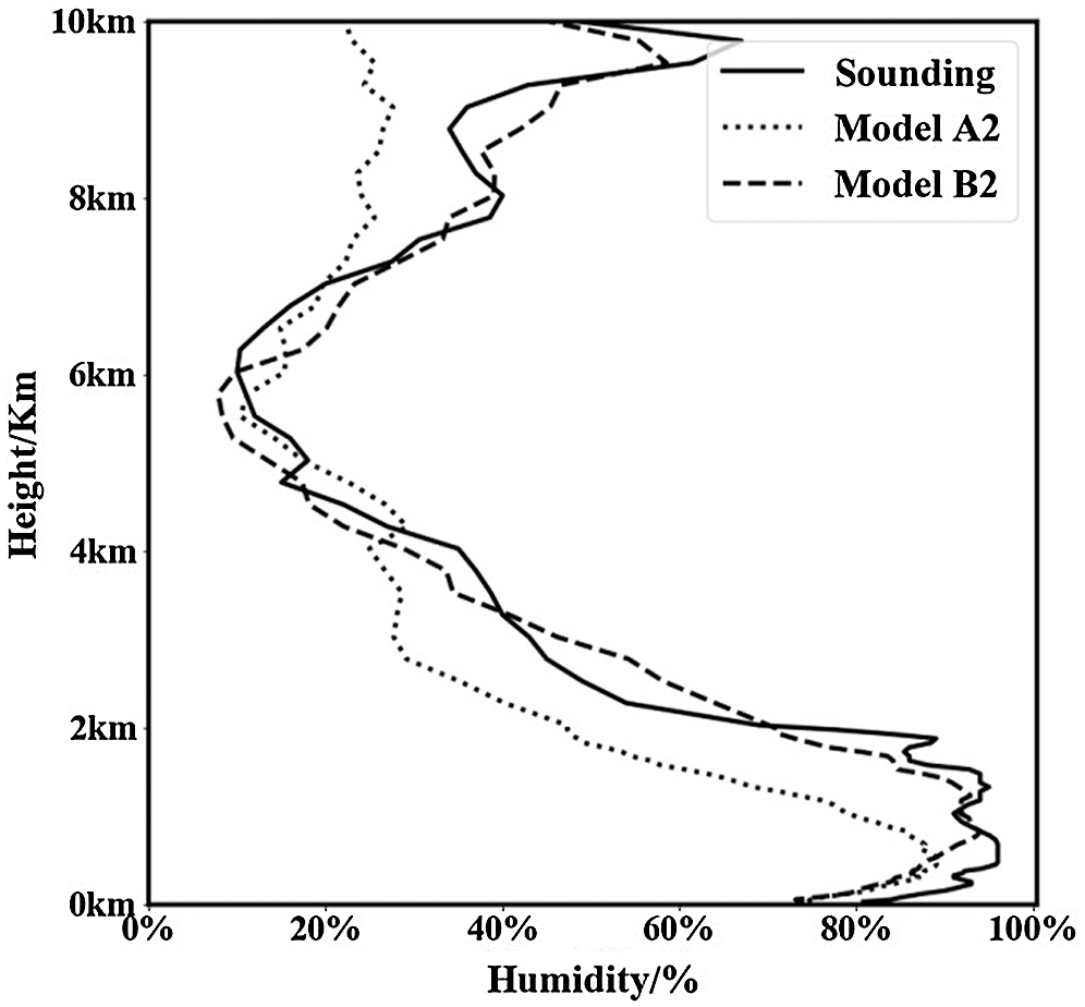
Figure 6: Comparison of atmospheric humidity profiles under cloudy weather
Fig. 7 presents the root mean square error chart of sunny weather samples from July 1, 2019 to September 10, 2019. Based on the humidity value of the actual sounding data, the root mean square error of humidity results inverted by models A2 and B2 with the actual value calculated at each altitude level. As can be seen from the figure, the RMSE of model B2 is significantly lower than that of model A2: the average RMSE of model A2 is 9.8%, and that of model B2 is 4.6%. For each altitude level, the RMSE of model A2 (without cloud information) increased rapidly from 3% to 13% within 0–2 km, while the RMSE of model B2 was stable at about 4%, and the highest RMSE was only 5.1%. At an altitude of 2–4 km, the RMSE of both models increased, with the highest RMSE of 16.2% for model A2 and 9.2% for model B2; the effect of the latter was better. At a height of 4–6 km, the prediction results of the two models are close, with average RMSE of 11.3% and 8.4% respectively. At altitudes above 6km, moreover, the RMSE of Model A2 is again significantly higher than that of Model B2, while the average error of the former reaches 10.8%, which is much higher than the latter’s 4.6%. As the altitude increases, the RMSE of the two gradually decreases. At 10 km, the RMSE of Model A2 is 6.3% and that of Model B2 is 2.7%. This phenomenon is consistent with the individual case in Fig. 5. At the medium altitude level, it can be seen that the prediction effects of the two models are similar, while at low and high altitudes, the prediction effect of Model B2 (with added cloud information) remains stable; this is a significant improvement compared with the model without cloud information. Fig. 8 presents the root mean square error chart of cloudy samples from July 1, 2019 to September 10, 2019. Based on the humidity value of the actual sounding data, the root mean square error of the humidity results inverted by model A2 and model B2 is calculated with the actual value at each altitude level. As can be seen from the figure, compared with the sunny samples in Fig. 7, due to the influence of clouds on humidity, RMSE in cloudy conditions is significantly increased. The average RMSE of model A2 reaches 13.6%, while that of model B2 reaches 8.9%, which is generally higher than that under sunny conditions. Through case analysis and statistical analysis, it can be seen that when clouds are present, the inversion difficulty of the humidity profile increases, and the prediction result of model A2 (without cloud information) deviates from the actual value; moreover, the inversion error of cloud layer and cloud height will evidently increase. B2 (the model with cloud information added) can suppress this error and obtain relatively stable and real prediction results, which is helpful in improving the inversion accuracy of a microwave radiometer under cloud conditions.
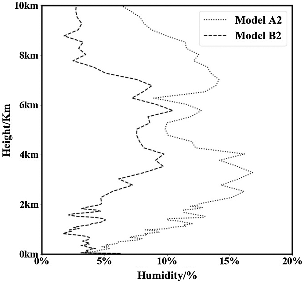
Figure 7: MSE comparison of atmospheric humidity profile inversion results under sunny weather
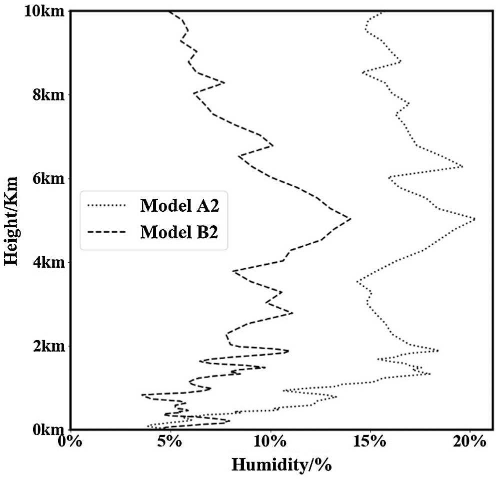
Figure 8: MSE comparison of atmospheric humidity profile inversion results under cloudy weather
In this paper, four network models for the inversion of atmospheric temperature and humidity profiles using microwave radiometer brightness temperature data are trained using sounding data obtained by the China Meteorological Administration from July 2018 to June 2019, combined with the MonoRTM radiation transfer model and BP neural network inversion algorithm. The model is evaluated and tested using Level 1 microwave radiometer data and millimeter wave cloud radar data from July 2019 to September 2019. The sounding data are used as the reference standard. After comparing several groups of experiments, the following conclusions can be drawn. In the entire troposphere, the inversion results of the two temperature models are found to be in good agreement with the measured values in clear weather. The average errors between the two models and the measured values are only 0.62°C and 0.45°C respectively, with these values increasing to 1.74°C and 0.97°C under cloudy conditions. Compared with sunny days, the inversion is more difficult and the effect is worse under cloudy conditions. The error of model A1 (without cloud information) increases by 1.12°C under these conditions, while that of model B1 (with cloud information) increases by 0.52°C, representing an improvement compared with model A1. This phenomenon is in line with expectations. Due to the influence of the cloud layer, the instability of the atmospheric temperature increases and the difficulty of inversion also increases. However, model B1 (with cloud information) is better able to adapt to this change. The inversion of the humidity profile is more difficult relative to the temperature profile. The results show that the variation trend of the two humidity models is similar to that of the sounding measured humidity profiles, but the accuracy is not high: the average errors between the two models and the measured values are 9.8% and 4.6% respectively. Similar to the inversion results of the temperature profile, the accuracy of the humidity profile will decrease under cloudy conditions, while the average error between the two models and the measured value increases to 13.6% and 7.58%. On the whole, model B2 (with cloud information) improves the accuracy of humidity profile inversion. Model A2 (without cloud information) exhibits a significant decline in layers with cloud, while model B2 remains stable; the latter model can thus effectively improve the prediction accuracy, with an average error reduction of 4% ~ 5%.The results show that the BP neural network can both feasibly and effectively invert the atmospheric temperature and humidity profiles. The temperature and humidity profiles obtained via inversion exhibit a good prediction trend and prediction accuracy. In addition, adding cloud information in the process of inverting atmospheric temperature and humidity profiles helps to improve the inversion accuracy and prediction effect, particularly in layers with cloud. Due to the lack of microwave radiometer and cloud radar data, as well as the imperfection of data quality control methods, the number of validation samples is small and invalid data points are present, which may affect the inversion results. In future research and testing work, we will increase the number of samples, improving the methods of data quality control for microwave radiometer and cloud radar data, thereby improving the accuracy of the inversion of atmospheric temperature and humidity profiles.
Funding Statement: This research was supported by the National Natural Science Foundation of China under Grant Nos. 61772280 and 62072249.
Conflicts of Interest: The authors declare that they have no conflicts of interest to report regarding the present study.
1. Z. G. Liu, “Using VHF radar to determine the height of troposphere and retrievefig temperature profile,” Meteorological Technology, vol. 13, no. 1, pp. 90–92, 1985. [Google Scholar]
2. Z. H. Wang, “A numerical experiment of the atmospheric temperature profile inversion from satellite-based amsu measurements through the improved of approach,” Journal of Nanjing Institute of Meteorology, vol. 13, no. 3, pp. 410–416, 1990. [Google Scholar]
3. X. B. Wu, F. Y. Zhang and Y. J. Zhu, “Inversion of atmospheric parameters using hyperspectral infrared data,” Meteorological Technology, vol. 31, no. 4, pp. 201–205, 2003. [Google Scholar]
4. C. H. Dong, J. Yang, N. M. Lu, Z. D. Yang, J. M. Shi et al., “Main characteristics and primary applications of polar-orbiting satellite FY-3A,” Journal of Geo-information Science, vol. 12, no. 4, pp. 458–465, 2010. [Google Scholar]
5. A. M. Zhang, “Atmospheric temperature and humidity profiles inversion from hyperspectral infrared simulation data based on FY 4, dissertation,” Nanjing University of Information Technology, 2017. [Google Scholar]
6. Y. H. Guan, J. Ren, Y. S. Bao, Q. F. Lu, H. Liu et al., “Research of the infrared high spectral (IASI) satellite remote sensing atmospheric temperature and humidity profiles based on the one-dimensional variational algorithm,” Transactions of Atmospheric Sciences, vol. 42, no. 4, pp. 602–611, 2019. [Google Scholar]
7. J. I. H. Askne and E. R. Westwater, “A review of ground-based remote sensing of temperature and moisture by passive microwave radiometers,” IEEE Transactions on Geoscience and Remote Sensing, vol. GE-24, no. 3, pp. 340–352, 1986. [Google Scholar]
8. A. Chedin, N. A. Scott, C. Wahiche and P. Moulinier, “The improved initialization inversion method: A high resolution physical method for temperature inversions from satellites of the TIROS-N series,” Journal of Climate and Applied Meteorology, vol. 24, no. 2, pp. 128–143, 1985. DOI 10.1175/1520-0450(1985)024<0128:TIIIMA>2.0.CO;2. [Google Scholar] [CrossRef]
9. Z. H. Wang and E. R. Westwater, “Using microwave radiometer and radar to jointly retrieve atmospheric temperature distribution,” Transactions of Atmospheric Sciences, vol. 9, no. 3, pp. 291–298, 1986. [Google Scholar]
10. H. Y. Liu, “The temperature profile comparison between the ground-based microwave radiometer and the other instrument for the recent three years,” Acta Meteorologica Sinica, vol. 69, no. 4, pp. 719–728, 2011. [Google Scholar]
11. X. L. Wang, J. K. Wang and J. Li, “Research for microwave radiometer remote sensing inversion of temperature and humidity profiles,” Meteorological Hydrological and Marine Instruments, vol. 29, no. 4, pp. 1–6, 2012. [Google Scholar]
12. J. L. Sanchez, R. Posada and E. Garcia-Ortega, “A method to improve the accuracy of continuous measuring of vertical profiles of temperature and water vapor density by means of a ground-based microwave radiometer,” Atmospheric Research, vol. 122, no. 2-4, pp. 43–54, 2013. [Google Scholar]
13. Q. Tan, Z. G. Yao, Z. L. Zhao, Z. G. Han, X. J. Sun et al., “Analysis of atmospheric parameter inversions from airborne microwave sounding instruments,” Meteorological Hydrological and Marine Instruments, vol. 31, no. 3, pp. 5–11, 2014. [Google Scholar]
14. N. Li, W. Zhang, Y. Chen, D. Liu, J. S. Shi et al., “Remote sensing detection of atmospheric temperature and humidity profile based on microwave radiometer,” Journal of Lanzhou University (Natural Sciences), vol. 51, no. 1, pp. 61–71, 2015. [Google Scholar]
15. J. J. Mao, X. F. Zhang, Z. C. Wang, R. K. Yang, X. G. Pan et al., “Comparison of brightness temperature accuracy of multi-model ground-based microwave radiometers,” Journal of Applied Meteorological Science, vol. 29, no. 6, pp. 724–736, 2018. [Google Scholar]
16. C. Z. Wu, J. Q. Hu and Q. H. Li, “Microwave radiometer MP3000A inversion error analysis,” Automation Application, vol. 24, no. 5, pp. 57–58, 2019. [Google Scholar]
17. H. H. Xu, X. F. Zhang, S. Y. Huang and W. Z. Fu, “Comparative analysis of ground-based microwave radiometer and UAV sounding observation,” Bulletin of Science and Technology, vol. 36, no. 1, pp. 48–53, 2020. [Google Scholar]
18. M. Montopoli, A. D. Carlofelice and M. Cicchinelli, “Lunar microwave brightness temperature: Model interpretation and inversion of spaceborne multifrequency observations by a neural network approach,” IEEE Transactions on Geoscience and Remote Sensing, vol. 49, no. 9, pp. 3350–3358, 2011. [Google Scholar]
19. L. Yang and L. Guan, “Study on the inversion of clear sky atmospheric humidity profiles with artificial neural network,” Meteorological Monthly, vol. 37, no. 3, pp. 18–324, 2011. [Google Scholar]
20. X. Y. Huang, X. Zhang, L. Leng, F. Li and Y. W. Fan, “Study on inversion methods with MonoRTM for microwave radiometer measurements,” Journal of the Meteorological Sciences, vol. 33, no. 2, pp. 138–145, 2013. [Google Scholar]
21. Y. S. Bao, Calx and Qlanc, “0~10 km temperature and humidity profiles inversion from ground-based radiometer,” J Trop Meteor, vol. 24, no. 2, pp. 243–252, 2018. [Google Scholar]
22. D. Q. Gao, “Research on the structure of linear basic function forward neural network with teachers,” Chinese Journal of Computers, vol. 21, no. 1, pp. 80–86, 1998. [Google Scholar]
23. K. D. Poore, “Top and thickness climatology from RAOB and surface data,” Cloud Impacts on DOD Operations and Systems Conference, 1991. [Google Scholar]
24. K. D. Poore, J. H. Wang and W. B. Rossow, “Cloud layer thicknesses from a combination of surface and upper-air observations,” JClimate, vol. 8, no. 3, pp. 550–568, 1995. [Google Scholar]
25. J. J. Mao, X. F. Zhang and Z. C. Wang, “Comparison of brightness temperature accuracy of multi-model ground-based microwave radiometers,” Journal of Applied Meteorology, vol. 29, no. 6, pp. 724–736, 2018. [Google Scholar]
 | This work is licensed under a Creative Commons Attribution 4.0 International License, which permits unrestricted use, distribution, and reproduction in any medium, provided the original work is properly cited. |