Intelligent Automation & Soft Computing DOI:10.32604/iasc.2021.018190
Article

A Hypergraph-Embedded Convolutional Neural Network for Ice Crystal Particle Habit Classification

Mengyuan Liao1, Jing Duan2,3,*, Rong Zhang2,3, Xu Zhou2,3, Xi Wu1, Xin Wang4 and Jinrong Hu1

1School of Computer Science, Chengdu University of Information Technology, Chengdu, 610000, China
2State Key Laboratory of Severe Weather, Chinese Academy of Meteorological Sciences, Beijing, 100081, China
3Key Laboratory for Cloud Physics of China Meteorological Administration, Chinese Academy of Meteorological Sciences, Beijing, 100081, China
4Keya Medical, Seattle, WA, 98104, USA
*Corresponding Author: Jing Duan. Email: duanjing@cma.gov.cn
Received: 28 February 2021; Accepted: 02 April 2021

Abstract: In the field of weather modification, it is important to accurately identify the ice crystal particles in ice clouds. When ice crystal habits are correctly identified, cloud structure can be further understood and cloud seeding and other methods of weather modification can be used to change the microstructure of the cloud. Consequently, weather phenomena can be changed at an appropriate time to support human production and quality of life. However, ice crystal morphology is varied. Traditional ice crystal particle classification methods are based on expert experience, which is subjective and unreliable for the identification of the categories by threshold setting. In addition, existing deep learning methods are faced with the problem of improving classification performance on datasets with unbalanced sample distributions. Therefore, we designed a Convolutional Neural Network (CNN) embedded with a hypergraph convolution module, named Hy-INet. The hypergraph convolution module can effectively capture information from hypergraphs constructed from local and global feature spaces and learn the features of small samples in ice crystal datasets that have unbalanced sample numbers. Experimental results demonstrate that the proposed method can achieve superior performance in the classification task of ice crystal particle habits.

Keywords: Classification; ice crystal particle; CNN; hypergraph

1  Introduction

The phase states of clouds are usually divided into ice clouds, water clouds, and mixed clouds. Ice clouds and mixed clouds are critical cloud systems that produce precipitation, and the frequency at which they occur is closely related to the frequency and amount of precipitation. Under different humidity, temperature, and environmental conditions, ice clouds are mainly composed of numerous different shapes and sizes of ice crystal particles. After obtaining accurate ice particle habits, we can further calculate the physical properties of ice clouds and mixed clouds, such as cloud liquid water content and the scale and concentration of ice crystal particles. Through a better understanding of the physical properties of ice clouds and mixed clouds, we can better understand the cloud microphysical process, decide the cloud seeding time, and evaluate the cloud seeding effect including precipitation enhancement and hail suppression. Thus, it is of great importance to accurately classify ice crystal particle images for research on cloud microphysics and weather modification.

In the past, the classification methods for ice crystal particles were all based on expert experience. Traditional methods require considerable time and effort and rely on much subjective empirical knowledge, which leads to inconsistencies and deviations. In addition, traditional methods of automatic classification of ice crystal particles are based on ice crystal particle physical properties, such as particle radius and circumference, to distinguish different categories, such as statistical recognition methods based on probability [1–3] and parameter identification methods based on particle image geometric characteristics [4,5]. Traditional physical methods are classified according to threshold setting and the subjective experience of experts. However, due to the different geographical and climatic conditions, the physical properties of ice crystal particle characteristics are variable. The threshold method will lead to inconsistent classification results and low prediction accuracy. Therefore, it is of great practical significance to use computer vision technology to solve practical weather tasks and realize high-precision automatic classification of ice crystal particles.

In recent years, deep learning has demonstrated excellent performance in the computer vision field, especially in image classification tasks, achieving extremely high accuracy. In 2012, the Convolutional Neural Network (CNN) AlexNet model, proposed by Krizhevsky et al. [6], made a historic breakthrough in the image classification task and significantly exceeded traditional methods. After that, as the model became deeper, a series of classic models [7–10] for image classification emerged. In the field of weather, Wang et al. [11] used lightweight convolutional neural networks to realize the recognition of weather phenomena. To the best of our knowledge, TL-ResNet152 [12], which is the first and only method to perform ice crystal classification using the deep learning method and CNN, has achieved good results. However, due to the variety of weather conditions and ice crystal morphology, the data for different categories in the ice crystal dataset will be unbalanced. The excellent performance of the traditional CNN is based on rich data, so the performance of the model on unbalanced datasets can be further improved, especially for categories with fewer data.

In addition, graph-based methods [13–18] have received a great deal of attention. Since the connection between each node is not fixed, it can be determined by our specific task characteristics. By calculation, we can connect the more similar vertices in the graph and can better capture the internal dependencies of data. Compared with the fixed-size convolution window in CNNs, the Graph Convolutional Neural Network (GCN) [19] can better capture the relationship between remote vertices to obtain more information and improve the model's classification accuracy.

Furthermore, we adopted hypergraphs [20]. Compared with regular graphs, hyperedges in hypergraphs can connect any number of vertices, enhancing the diversity of feature relationships. The hyperedge is used to connect the central vertex and the adjacent related vertex to obtain deeper characteristic information, which is also helpful for unbalanced sample learning. At the same time, during the training process, the hypergraph structure can be dynamically modified by adjusted feature embedding [21] so that the hypergraph features can be extracted better according to relevant tasks. Therefore, we propose a hypergraph convolution module. In this module, we use a hypergraph convolutional layer and combine local and global context relations to construct hyperedges, which is beneficial to our classification task. Since the CNN has good classification performance and embedding a GCN into a CNN can effectively extract more feature information to improve performance [22], we propose a CNN embedded with our hypergraph convolution module for ice crystal particle classification called Hy-INet.

An overview of our proposed model Hy-INet is shown in Fig. 1. The convolutional layers before the hypergraph convolutional layers can be regarded as a graph feature extraction module. We construct the hypergraph from the local and global feature space on the convolutional layer’s feature map output. Next, we input the constructed hypergraph into the hypergraph convolution module to obtain the graph structure features and convert the acquired feature map to the following convolutional layer’s desired size. Then, after the following learning by the convolutional layers, the model will output the predicted ice crystal particle category.

Figure 1: An overview of the network architecture of the Hy-INet model

There are two main key contributions of this paper:

1.    Based on transfer learning, we propose a convolutional neural network embedded with hypergraph convolution to realize automatic classification of ice crystal particles.

2.    We propose a hypergraph convolution module that combines global and local relations to construct hypergraphs and can be effectively used for ice crystal particle classification.

2  Materials and Methods

In this section, we introduce the proposed Hy-INet model, which is composed of a CNN embedded with our proposed hypergraph convolution module. The experimental results have demonstrated that the proposed hypergraph convolution module can effectively obtain feature information from unbalanced samples, thus improving overall classification performance.

2.1 Network Structure

Fig. 2 illustrates the network structure of the Hy-INet model. To obtain characteristic information that cannot be captured by the traditional CNN, we embed the proposed hypergraph convolution module into a CNN. The hypergraph convolution module can help to improve the learning ability of the traditional CNN for unbalanced samples, which improves its performance in the ice crystal classification task.

Figure 2: The network architecture of the Hy-INet model

First, in the selection of the CNN, we choose the ResNet152 network, which uses a global average pooling layer (GAP) [23] and has the best performance on the ImageNet dataset. The traditional classification CNN usually uses two fully connected layers at the end of the network to output the final prediction results. In contrast, using a GAP layer to replace the fully connected layer commonly used in the CNN's penultimate layer can reduce the dimensions of the feature map and regularize the structure of the whole network to prevent overfitting.

Second, in the hypergraph convolution module, we first use the feature maps previously obtained from the traditional convolution layer to construct hypergraphs. Then, we use hypergraph convolution to update the pixel values according to the hypergraph structure. A more specific design and implementation of this module are as follows.

2.2 Hypergraph Convolution Module

The purpose of the proposed hypergraph convolution module is to explore more diverse and advanced feature information that cannot be obtained by the traditional CNN to improve the performance for ice crystal classification tasks. The design idea of the proposed hypergraph convolution module is as follows.

First, the inputs to the hypergraph convolution module are the feature maps with shape X ∈ RB*C*H*W obtained from the previous traditional convolution operation, where B, C, H and W represent the batch size, channel, height and width, respectively.

Second, according to the correlation between each vertex in the feature maps, we select vertices from local and global feature spaces to construct hyperedges and then construct hypergraphs (see Fig. 3). Then, we reshape the feature maps as X ∈ RN*C, where N and C represent the number of vertices and channels, respectively, and N = B*H*W.

Figure 3: Hypergraphs constructed from local and global feature spaces

Third, we input the reshaped X ∈ RN*C into the hypergraph convolutional layer and update the vertices according to the vertex and edge structure information in the constructed hypergraphs. This step can help to learn more characteristics of the higher-level information, which will not be captured by the traditional convolution.

Finally, after the hypergraph convolution operation is completed, we restore X ∈ RN*C to the input size format suitable for the following traditional convolutional layers, which require a shape of X ∈ RB*C*H*W.

In the hypergraph convolution module, each hypergraph convolutional layer is followed by a nonlinear activation function and a dropout. In practical applications, we can flexibly set the number of hypergraph convolutional layers. To be embedded into the CNN, the number of input channels of the first hypergraph convolution layer should be equal to the number of output channels in the previous traditional convolutional layer. The number of output channels of the last hypergraph convolution layer should be the same as the number of input channels in the following traditional convolutional layer.

Next, the method for constructing hypergraphs from the local and global feature space is introduced as follows.

2.2.1 Hypergraphs from the Local Feature Space

Due to the local self-similarity of the image, the pixels adjacent to a pixel are likely to have a greater correlation. Simultaneously, the most noticeable feature used to distinguish categories usually appears in a local area. The category of the image can be inferred by combining the contextual information of surrounding pixels with a central pixel point. To obtain more detailed information, we need to establish feature relationships in local space.

We choose a simple and effective way to build local relationships. We select the eight neighborhood pixels of the center pixel to form a hyperedge that represents the local space's characteristic relationship around the center pixel. Simultaneously, using the flexibility and diversity of hyperedges that can contain any number of vertices, we can construct hyperedges containing different numbers of vertices for central pixels at different positions. For the center pixels that are not at the boundary, each hyperedge has four adjacent horizontal and vertical pixels surrounding its center and four adjacent diagonal pixels with a total of eight vertices. For center pixels on the edge, each hyperedge contains five or three surrounding pixels.

2.2.2 Hypergraphs from the Global Feature Space

In addition to characterizing detailed features, a comprehensive analysis of the image is also crucial to classification. In general, the KNN (K nearest neighbors) method is typically used to calculate the distance between two pixels and to select the K global nearest pixels to the center vertex through similarity measurement.

Based on the KNN, we add the idea of the patch-based method. We believe that after a patch is added, more vertex information is used when constructing hyperedges, improving classification performance. We define an N × N patch centered on a vertex. We calculate the distance of two patches to represent the distance between vertexes corresponding to two centers. On this basis, we can obtain the distance between each vertex and other vertices and then select the KNN of the center vertex, thus constructing a hyperedge that contains a K+1 vertex including the center vertex.

2.2.3 Hypergraph Convolution

A hypergraph is defined as G=(V,E,W) , where V is the set of finite vertices of the hypergraph, E is the set of hyperedges of the hypergraph, and W is the weight matrix of the hyperedge. In a hypergraph, the degree of a vertex ν∈V is defined as follows:

dv(ν)=∑{ν∈e,e∈E}⁡w(e) (1)

where w(e) is the weight of the hyperedge e .

For the hyperedge e∈E , the degree of the hyperedge is defined as the number of vertices contained in the hyperedge:

de(e)=|e| (2)

We denote the diagonal matrix forms of dv(ν) and de(e) as Dv and De . Similar to the matrix representation of ordinary graphs, a hypergraph can also be represented by constructing a |V|×|E| dimensional point-side incidence matrix H , which is defined as follows:

h(ν,e)={1,ifv∈e0,otherwise (3)

According to the definition of the incidence matrix H , the degree of vertices and edges in the hypergraph can be further expressed as

dv(ν)=∑{ν∈e,e∈E}⁡w(e)=∑{e∈E}⁡w(e)h(ν,e) (4)

de(e)=|e|=∑{v∈e}⁡h(ν,e) (5)

According to the symmetric Laplacian operator, the convolution expression on the hypergraph structure can be obtained,

X(l+1)=σ(Dv−1/2HWDe−1H⊤Dv−1/2X(l)Θ(l)) (6)

where σ(.) denotes the nonlinear activation function and X(l) denotes the hypergraph vertex characteristic matrix, and the convolution expression can be operated by a learnable parameter matrix Θ(l) to obtain the features of a vertex in a deeper dimension. According to the symmetric normalized Laplacian operator and the previously introduced hypergraph adjacent matrix H , by combining the vertex degree matrix Dv and hyperedge degree matrix De with the hyperedge characteristics, we can obtain the vertex characteristic matrix of the next layer X(l+1) .

2.3 Objective Function

We use the cross-entropy loss function to learn to predict the ice crystal category. It mainly describes the distance between the actual output and the expected output, which is defined as follows:

H(p,q)=−∑i=0N⁡p(xi)log(q(xi)) (7)

where N is the number of samples; the probability distribution p is the expected output, namely, the real tag of the data; and q is the actual output, namely, the tag predicted by the model. The smaller the cross-entropy loss is, the closer the two distributions are, and the better the classification result is.

2.4 Implementation Details

First, in the hypergraph convolution module, when defining the hyperedge weight matrix W, since we cannot explicitly define an appropriate matrix W, we define the weight of each hyperedge as 1. When constructing the global hypergraph, we set the patch to 3 × 3 and select the three global nearest points of the central vertex to form the hyperedge containing four vertices, including the central vertex. In addition, we choose Leaky ReLU as the activation function, and we set the parameter P of the dropout layer to 0.3.

Second, in the CNN, due to the small amount of ice crystal data, some transfer learning methods [24,25] are usually selected to accelerate and optimize the learning efficiency and classification performance of the new model. Therefore, we choose fine-tuning methods [26,27] to use the pre-trained parameters to initialize the traditional convolutional layers.

Third, we found that when the hypergraph convolution module was embedded between Layer1 and Layer2 in the ResNet152 network and was using one hypergraph convolution layer, the prediction accuracy could be maximally improved.

3  Experiments

To illustrate the effectiveness and accuracy of the Hy-INet model, we carried out comparative experiments using various models with the same post-processing and the same experimental conditions on the same dataset. The experimental results were evaluated by the same standard. The models compared include VGG16 [7], DenseNet169 [10] and the ResNet152 [9] model.

3.1 Data

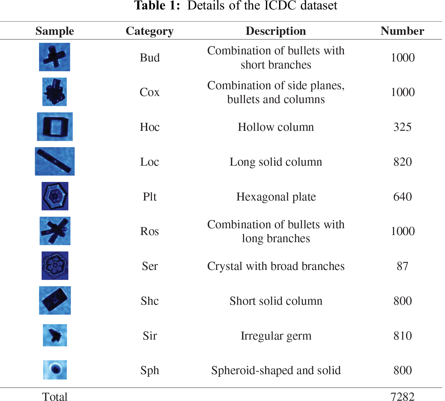
The data used in the experiments in this paper are based on the Ice Particle Database in China (ICDC) [12], which is a dataset of ice particle images with labels that are detected by the cloud particle imager (CPI) on an airplane in Hebei Province, China. The ICDC contains 7,282 images of ice crystals in the following ten categories: Budding Rosettes (Bud), Complex with Side Planes (Cox), Hollow Columns (Hoc), Long Columns (Loc), Plates (Plt), Rosettes (Ros), Sector Plates (Ser), Short Columns (Shc), Small Irregulars (Sir) and Spheroids (Sph). In this dataset, the data resolution varies, and each category contains a different number of samples. The lowest resolutions in the dataset are the Sir and Sph category, whose size is generally 39 × 35 pixels. The highest resolution image data are in the Cox category, which can reach 739 × 567 pixels. Among the ten categories, there are three categories (i.e., Bud, Cox and Ros) that contain the highest number of samples (each containing 1000 samples), while Ser has the lowest number of samples (only 87). See Tab. 1 for the specific category details.

3.2 Evaluation Metrics

To better evaluate the classification results of the Hy-INet model, we used accuracy to assess the overall classification results. Precision, recall, F1, precision-recall (PR) curve, average precision (AP) value, obfuscating matrix, receiver operating characteristic (ROC) curve, and the area under the curve of ROC (AUC) value were used to evaluate the classification results of each category.

Accuracy refers to the ratio between the number of samples correctly classified by the model and the total number of ice crystal images in a given training or test dataset, and it is defined as

Accuracy(y,y^)=1M∑i=0M⁡eq(yi,y^i) (8)

where y^i represents the tag value of the i-th image predicted by the model, yi is the corresponding true tag value, M is the total number of images input to the model, and eq(yi,y^i) is the equal function, which states that if and only if yi equals y^i , eq(yi,y^i) is equal to 1.

Precision (P) and recall (R) are calculated by TN (true negatives), TP (true positives), FN (false negatives), and FP (false positives). The definitions are as follows:

Pi=TPiTPi+FPi,Ri=TPiTPi+FNi (9)

where Pi and Ri represent the accuracy and recall of the i-th category, respectively. The F1 value is the harmonic mean value of P and R, and it is defined as follows:

F1i=21/Pi+1/Ri (10)

where F1i represents the F1 value of the i-th category.

Furthermore, the macro average values of P, R and F1 are calculated based on the whole result and are defined as follows:

Macro_P=1N∑i=1N⁡Pi,Macro_R=1N∑i=1N⁡Ri (11)

Macro_F1=1N∑i=1N⁡F1i (12)

The PR curve is derived from the horizontal axis, recall, and the vertical axis, precision. Recall reflects the classifier's ability to cover positive examples, precision reflects the precision of a classifier to predict positive examples, and the PR curve reflects the trade-off between the two. The AP value is the area under the PR curve, which is defined as follows:

AP=∫01⁡P(R)dR (13)

The ROC curve is calculated by the true positive rate (TPR) and the false positive rate (FPR). The closer the ROC curve is to the point (0,1), the better the classifier effect will be. TPR and FPR are defined as follows:

TPRi=TPiTPi+FNi,FPRi=FPiFPi+TNi (14)

where TPRi and FPRi represent the TPR and FPR values corresponding to the ROC curve of the i-th category, respectively.

The AUC value is the area under the ROC curve, which can be used to visually evaluate the quality of the classifier. The higher the AUC value, the better the performance of the classifier. The AUC definition is as follows:

AUC=∫01⁡TPR(FPR)dFPR (15)

3.3 Experimental Settings

To better analyze the performance of the proposed model and demonstrate its validity, we choose the same hyperparameters and dataset partitioning method as is used in the TL-ResNet152 model. We select approximately 20% of the data of each category in the ICDC dataset, a total of 1456 images, as the test set and the rest as the training set, ensuring that the training set data and the test set data do not overlap. Simultaneously, we enhance the input data, i.e., we randomly flip the original image horizontally and randomly sample the image to create an input image of size 224 × 224. In addition, to improve the generalization ability of the model, the dataset is also standardized by pixel. The pixel value of each channel in the image is subtracted from the mean value of the pixel value of the corresponding channel and then divided by the standard deviation to achieve data normalization. In the experiment, we calculate the mean value and standard deviation of different color channels in the training set and the test set to standardize the input data. The RGB channels' mean values in the training set are 0.035, 0.274 and 0.593, and the standard deviations are 0.069, 0.210 and 0.301, respectively. The mean values in the test set are 0.036, 0.279 and 0.600, and the standard deviations are 0.070, 0.211 and 0.301, respectively.

We choose the SGD optimizer to perform stochastic gradient descent to optimize the parameters and set its momentum parameter to 0.9. In addition, due to the small amount of training data, to improve the model's performance and optimize the learning efficiency, the parameters of the pre-trained ResNet152 model on ImageNet are used for the initialization of the corresponding convolutional layer of our model. The training process is set as 30 epochs, with an initial learning rate of 0.001 and a batch size of 8. The classification accuracy of the model is tested on the test set after each training epoch, and we save the model with the highest test accuracy.

We load three classic classification models, VGG16, DenseNet169, and ResNet152, which were also pre-trained on ImageNet. We change the output of the final fully connected layer to ten to correspond to the ten categories' predictions in our dataset. The above three models were trained with the same method on the same training set as the proposed model. The model that has the highest prediction accuracy of each model in the test set will be saved during the training process to be analyzed and compared.

3.4 Results and Discussion

We saved Hy-INet, VGG16, DenseNet169 and ResNet152 (which is used in TL-ResNet152 [12]) with the highest accuracy evaluated on the test set during the training process. We analyzed the prediction results of the four models on the test set.

Fig. 4 shows the confusion matrix of the four models' classification results on the test set, which has been standardized by row. The Hy-INet model can distinguish most categories of ice crystal images well, and the classification recalls of all categories are over 94%, with a low of 94.12% and a high of 100%. The lowest recalls of the TL-ResNet152, DenseNet169 and VGG16 models are 93.75%, 88.24% and 92%, respectively. There is no category that has 100% recall when tested on the DenseNet169 and VGG16 models. Simultaneously, the recall of the Hy-INet model was higher than that of the TL-ResNet152 model in all the other categories except Sir. It is also indicated that the performance of the Hy-INet model was superior to that of the TL-ResNet152 model in ice crystal classification.

Figure 4: Confusion matrix of the prediction maps of the four models on the test set

We evaluated the accuracy of the four models and the macro average values of precision, recall and F1 on the test set (see Tab. 2). We found that the accuracy of the Hy-INet model was 0.9808, higher than that of TL-ResNet152, which was 0.9753. At the same time, the Hy-INet model was superior to the other three models in terms of various evaluation metrics, which were all higher than 0.97. The evaluation metrics of VGG16, DenseNet169 and ResNet152 did not exceed 0.98. The macro-average value of R in the Hy-INet model was 0.9762, while the other metrics all exceeded 0.98. This indicates that our proposed Hy-INet model is effective and has good performance in the ice crystal classification task.

In addition, we further evaluated the test results in each category (see Tab. 3). Although the Ser category has the least sample data and only 70 images are used for training, the Hy-INet model's accuracy reaches 1.0. Both the recall and F1-score of Hy-INet are the highest values of the four methods. Moreover, we can see that the Hy-INet model obtains the highest value of F1-score for each category, and F1-score can weigh the values of P and R to better evaluate the classification model. All of the above results show that the proposed hypergraph convolution module has a good learning ability with a small sample, and the Hy-INet model has a good generalization ability.

We also analyzed and compared the PR and ROC curves of the four models (see Fig. 5). The area under the PR curve and area under the ROC curve are expressed as the corresponding AP value and AUC value, respectively. The larger their value is, the better the related classification effect will be. It is obvious that the AP value and AUC value obtained by the Hy-INet model are the highest both in macro- and micro-average value, which again indicates that the Hy-INet model has good performance in the ice crystal classification task.

Figure 5: Macro- and micro-average of PR and ROC curves

4  Conclusions

In this paper, we propose a Hy-INet model, which can effectively and accurately classify ice crystal particles on a class distribution imbalanced dataset. The key to this work is that we designed a hypergraph convolution module, which can effectively improve the model's classification accuracy on small samples. The experimental results show that the hypergraph convolution module can learn the feature information of a small sample of data well and achieves high precision on the ice crystal classification task. In the future, we will continue this work as follows: (1) We will expand the dataset further to improve the classification performance of ice crystal particles. (2) Based on the ice crystal particle category, we will further calculate clouds' physical properties, such as cloud liquid water content.

Funding Statement: This research was jointly funded by the National Key R&D Program of China (grant number 2018YFC1505702); the National Natural Science Foundation of China (grant number 41675137, 42075142); the Sichuan Science and Technology Program (grant number 2019ZDZX0005, 2019YFG0496); and the project of scientific research on weather modification in Northwest China, research for experiment design and application integration (RYSY201909).

Conflicts of Interest: The authors declare that they have no conflicts of interest to report regarding the present study.

This work is licensed under a Creative Commons Attribution 4.0 International License, which permits unrestricted use, distribution, and reproduction in any medium, provided the original work is properly cited.