Intelligent Automation & Soft Computing DOI:10.32604/iasc.2021.018338
Article

Optimization for Variable Height Wind Farm Layout Model

Bin Xu1,2,3,*, Jianming Zhu1, Junzhe Wen1, Shanshan Lin1, Yunkai Zhao1, Jin Qi1,2, Yu Xue4 and Sichong Qin5

1Nanjing University of Posts and Telecommunications, Nanjing, 210003, China
2Nanjing Pharmaceutical Co., Ltd., Nanjing, 210012, China
3Jiangsu Key Laboratory of Data Science and Smart Software, Jinling Institute of Technology, Nanjing, 211169, China
4School of Computer and Software, Nanjing University of Information Science and Technology, Nanjing 210044, China
5Central Washington University, Ellensburg 98926, United State
*Corresponding Author: Bin Xu. Email: xubin2013@njupt.edu.cn
Received: 03 March 2021; Accepted: 05 April 2021

Abstract: The optimization of wind farm layouts is very important for the effective utilization of wind resources. A fixed wind turbine hub height in the layout of wind farms leads to a low wind energy utilization and a higher LCOE (levelized cost of electricity). WOMH (Wind Farm Layout Optimization Model Considering Multiple Hub Heights) is proposed in this paper to tackle the above problem. This model is different from the traditional fixed hub height model, as it uses a variable height wind turbine. In WOMH, the Jensen wake and Weibull distribution are used to describe the wake effect on the wind turbines and wind speed distribution, respectively. An algorithm called DEGM (differential evolution and greedy method with multiple strategies) is proposed to solve WOMH, which is NP hard. In the DEGM, seven strategies are designed to adjust the distribution coordinates of wind turbines so that the height of the wind turbines will be arranged from low to high in the wind direction. This layout reduces the Jensen wake effect, thus reducing the value of the LCOE. The experimental results show that in the DEGM, when the number of wind turbines is 5, 10, 20, 30 and 50, the WOMH reduces the LCOE by 13.96%, 12.54%, 8.22%, 6.14% and 7.77% compared with the fixed hub height model, respectively. In addition, the quality of the solution of the DEGM is more satisfactory than that of the three-dimensional greedy algorithm and the DEEM (differential evolution with a new encoding mechanism) algorithm. In the case of five different numbers of wind turbines, the LCOE of DEGM is at least 3.67% lower than that of DEEM, and an average of 6.83% lower than that of three-dimensional greedy. The model and algorithm in this paper provide an effective solution for the field of wind farm layout optimization.

Keywords: Optimization of wind farm layout; variable multiple hub heights; differential evolution; Jensen wake model

1  Introduction

Air pollution, climate warming, the energy crisis and other factors are forcing people to find and develop clean energy that can replace fossil fuels. Wind energy is pollution-free and renewable and is currently one of the most competitive and mature green energy sources [1].

The main form of wind energy utilization is to generate electricity through wind farms [2]. Wind turbines are the core equipment used in wind farms to convert wind energy into electricity. The layout of a wind farm has a great impact on the wind turbines. There are three factors that affect the layout of wind farms: the size of the wind farm, the number of wind turbines placed in the wind farm, and the wake effect of upstream wind turbines on downstream wind turbines [3]. The focus of this research is how to eliminate the wake effect between wind turbines. A reasonable layout of wind turbines in wind farms can effectively reduce the wake effect, and a good wind farm layout can improve the power of wind turbines to make better use of wind energy resources.

The layout models of existing wind farms fall into two categories: discrete coordinate models and continuous coordinate models. The discrete coordinate model regards wind turbines as independent and scattered points for layout optimization. In the continuous coordinate model, the wind turbine can be placed anywhere in the wind farm. Because these two models are difficult to solve analytically and have a large amount of computations, many heuristic algorithms have been designed to solve the models. Mosetti et al. [4] proposed a model based on discrete coordinates and used a genetic algorithm to deter- mine the optimal solution. Considering the wake effect of wind farms, a wind farm cost model was designed that takes the LCOE (levelized cost of electricity) generated by the wind farm as the objective function. Three kinds of wind scenarios were assigned in the experiment: scenario 1-the wind direction and speed are constant; scenario 2-the wind speed is constant, and the wind direction is uniformly distributed between 0 and 360 degrees; scenario 3-the wind speed is variable, and the wind direction is uneven. Kusiak et al. [5] developed a continuous coordinate model and used the SPEA algorithm to solve the problem. They regarded individual wind turbines as a population, so when the number of wind turbines increases, the performance of the algorithm will be seriously degraded, and there may even be dimensional disasters. Subsequently, many researchers [6–10] studied different heuristic algorithms to solve the model based on continuous coordinates. Wang et al. [11] proposed a DE (differential evolution) algorithm with a new coding mechanism, which reduced the dimension of the search space to 2 and eliminated a key parameter (population size), thus solving the dimensional disaster problem.

However, only wind turbines with the same height are considered in the above studies. In practice, due to terrain or other reasons, the hub heights of wind turbines will differ. At the same time, different hub heights also help to further reduce the wake effect of the whole wind farm. In previous research, many scholars have discussed the multiple hub height model. Herbert et al. [12] placed wind turbines with two different heights in a line. The results showed that the use of wind turbines of different heights is beneficial for improving the power generation of wind farms. Chowdhury et al. [13] and Long et al. [14] used particle swarm optimization to optimize the multiple hub height model. The experimental results showed that the multiple hub height model can significantly increase the power output of the wind farm. Chen et al. [15] made use of greedy algorithm to solve wind turbines with different hub height models. In an experiment based on three-dimensional coordinates, two kinds of wind turbines with different hub heights were used. Then, two planes in three-dimensional coordinates were used as the candidate positions of the wind turbines. All of their results showed that the existence of wind turbines with different heights in a wind farm is beneficial for improving the power generation of the wind farm.

A wind farm layout optimization model considering multiple hub heights is studied in this paper. The DEGM (differential evolution and greedy method with multiple strategies) is proposed in this paper to solve the optimization problem. The complex terrain problem is studied and optimized in an experiment, and the advantages of using multiple hub height wind turbines in wind farms are further studied.

The main contributions of this paper are summarized as follows:

In the process of solving the actual wind farm layout, it is determined that wind turbines with multiple hub heights can effectively reduce the wake effect between wind turbines. In this paper, a novel model named WOMH (wind farm layout optimization model considering multiple hub heights) is designed to simulate the optimized layout of wind farms with multiple hub heights.

A series of adjustment strategies are proposed in the DEGM. These strategies integrate the position and height information of wind turbines so that the wind turbines are arranged in linear with a high probability to reduce the LCOE, and thus to improve the wind farm layout.

The remainder of this article is organized as follows. The second section introduces WOMH, and the specific details of the DEGM are described. The third part describes the experiment and data analysis. The fourth part summarizes the paper.

2  System Model

WOMH takes LCOE as the optimization goal. It contains three submodules: Jensen wake, Weibull distribution and output power. Jensen wake and Weibull distribution are used to describe the wake effect between wind turbines and wind speed distribution respectively. The output power model is made use of quantifying the output power.

2.1 The Jensen Wake Model

The Jensen wake model [16] is a one-dimensional wake model suitable for flat terrain. Fig. 1 depicts the Jensen wake model. In the model, v0 is the natural incoming wind speed, vr is the wind speed when the wind passes through the front turbine rotor, v is the incoming wind speed at the rear exhaust turbine affected by the wake, x is the distance between the front and rear exhaust turbines, R1 is the initial radius of the wake area, and Rw is the wake influence radius.

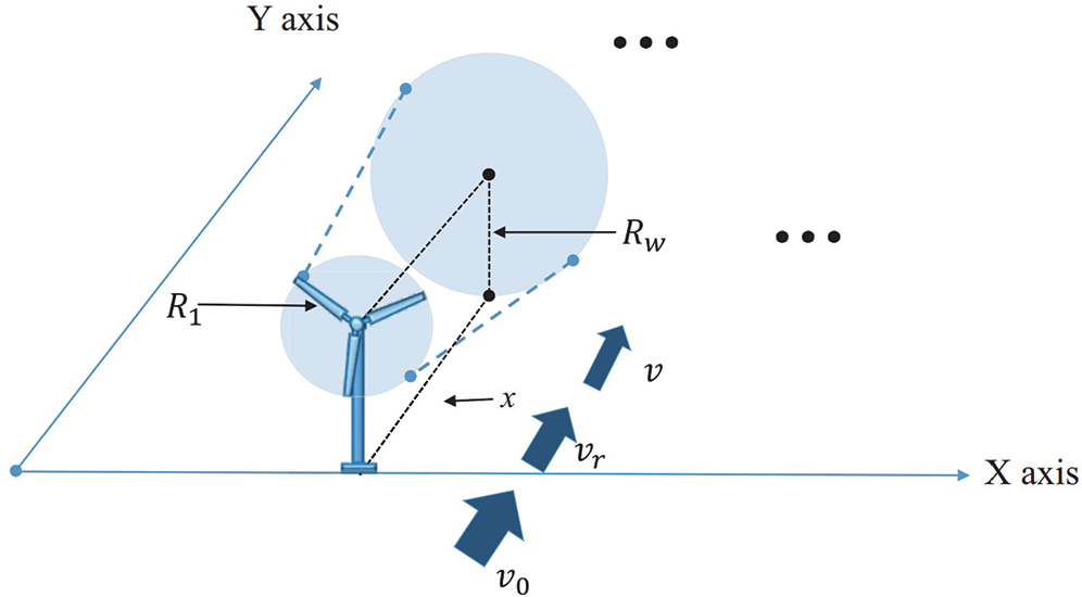
Figure 1: The Jensen wake model

The wind speed v in the downstream wake region is computed by (1):

v=v0[1−2t(1+kxRw)2], (1)

where k is the expansion rate of the wake area radius. k is related to the height, calculated by (2):

k=0.5ln(Hn0), (2)

where H is the height of the wind turbine, n0 is the roughness of the ground.

Rw is calculated by (3):

RW=R1+kx (3)

t is the axial induction factor, as shown in (4)

t=1−1−gT2, (4)

where gT is a fixed thrust coefficient [17,18].

2.2 Output Power Model

The wind turbine output power is related to the wind speed at the wind turbine wheel, Pi [19] is calculated by (5):

Pi=f(v)={0,vo≤v,v<vievα+βev,vi≤v<vrPrate,vr≤v≤vo, (5)

where Pi represents output power of the wind turbine i . α and β are the limiting parameters. vi , vo and vr represent cut-in speed, cut-off speed and rated speed, respectively. When vi is faster than v , energy cannot be extracted from the natural wind. When vo less than the wind speed v , the wind turbine will cut off and protect itself. If v is between the rated speed vr and vo , the wind turbine will sustain the rated output power Prate .

2.3 Weibull Distribution

To use the Jensen wake model, the wind farm is set up on a flat area. The wind turbines can always keep the rotation plane perpendicular to the wind direction by turning their nacelles. The wind direction is γ , and the wind speed is v which follows Weibull distribution. The probability distribution function [11] is (6):

ω(v,ci(γ),ki(γ))=ki(γ)ci(γ)(vci(γ))ki(γ)−1×e−(vci(γ))ki(γ),0∘≤γ<360∘, (6)

where ki(γ) is the shape parameter and ci(γ) is the scale parameter respectively.

2.4 Wind Farm Layout Model

2.4.1 Average Output Power of the Wind Turbines

The average output power E(Pi) [11] of wind turbine i can be obtained as (7):

E(Pi)=∫0∘360∘ω(γ)∫0∞f(v)ki(γ)ci,(γ)(vci,(γ))ki(γ)−1×e−vki(γ)ci,(γ)dvdγ, (7)

where ci,(γ) is the scale parameter modified by the wake effect.

2.4.2 The Layout Model of the Wind Farm

In optimizing the layout of wind farms, it is hoped that the total power output can be maximized while the cost can be minimized. Therefore, LCOE [20] is used as the evaluation function, as computed by (8):

LCOE=∑iN(CostH×Hi+Costb)∑i=1NE(Pi), (8)

where Costb is the basic cost of a wind turbine and CostH is the additional cost per unit height of the wind turbine, including the cost of cables and materials. The total number of wind turbines is N , and Hi represents the height of the wind turbine i .

The LCOE is the target of optimization in WOMH. In three-dimensional coordinates, the position of each wind turbine must ensure that the impeller does not cross the boundary and that the distance between two random wind turbines must be not less than five times the radius of the turbine impeller, that is, 5R. LCOE and its constraints are shown in (9):

{minimize:LCOE=∑iN(CostH×Hi+Costb)∑i=1NE(Pi)subjectto:(xj−xi)2+(yj−yi)2+(zj−zi)2≥5R,R≤xi≤x¯−R,R≤yi≤y¯−R,i=1,2,…,N,j=1,2,…,Nandj≠i. (9)

Suppose the coordinates of wind turbines i and j are (xi,yi,zi) , and (xj,yj,zj) , respectively, where x¯ and y¯ are the upper bounds of the wind farm. In WOMH, x , y , z are all continuous variables. Where z represents the height of the wind turbine, and its value range is [50,80].

2.5 DEGM Algorithm

In view of the variable hub height of wind turbine in WOMH, DEGM is proposed to solve this model. Before the advent of DEGM, many algorithms updated the coordinates of wind turbines in a way that was passive. Most of these algorithms use crossover, mutation or traversal when updating wind turbine coordinates. None of these methods is very purposeful. But DEGM is a purposeful algorithm. The DEGM not only integrates heuristic algorithms, such as DE and greedy algorithm, to balance the global search and local search capabilities but also adds six adjustment strategies to further improve the LCOE. In addition, a parameter adaptive mechanism [21,22] is introduced to give the DEGM a good robustness and ensure the quality of the solution. DEGM flowchart is shown in Fig. 2.

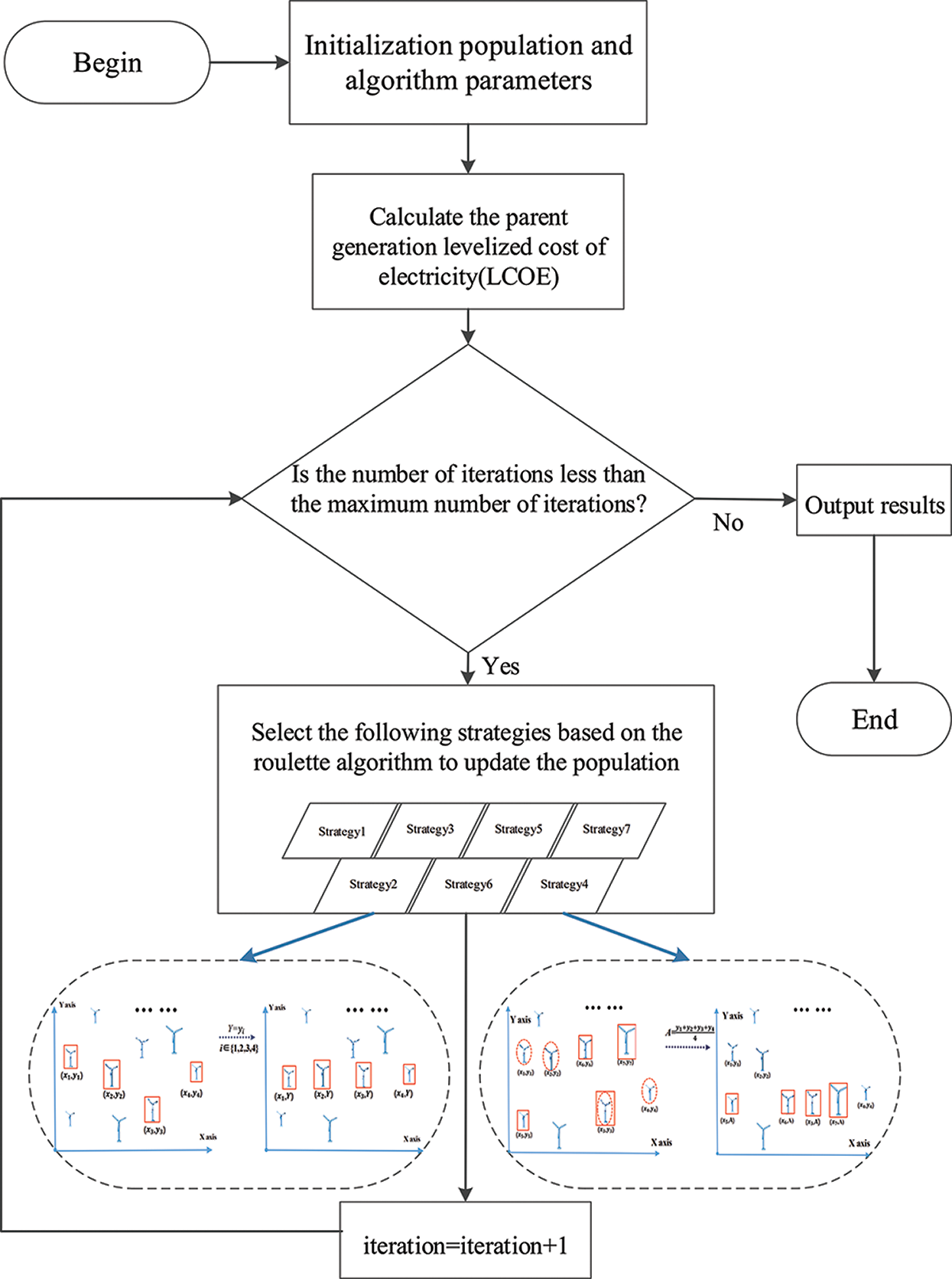
Figure 2: DEGM flowchart

2.5.1 Seven Strategies

Seven adjustment strategies are the core of the DEGM, which can adjust the positions of wind turbines to optimize LCOE. The following are the details of the seven adjustment strategies:

Strategy 1: Update the positions of wind turbines based on DE and greedy algorithm.

Strategy 2: Randomly select n wind turbines in the wind farm and set Y to the value of the y coordinates of one of the wind turbines. Then, the y coordinates of the n wind turbines are all set to Y . Strategy 2 is shown in Fig. 3.

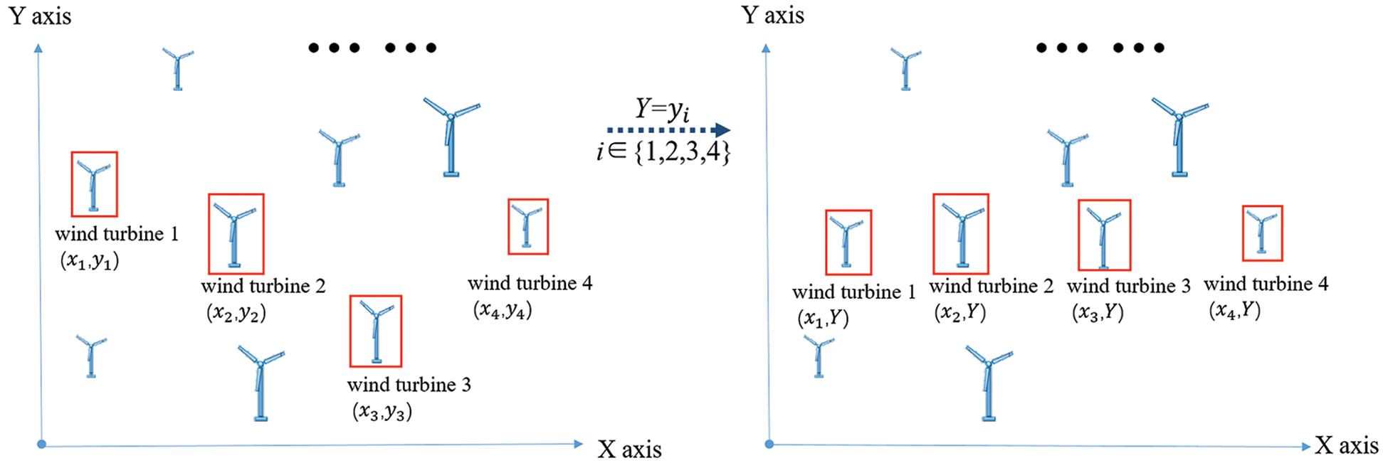
Figure 3: Strategy 2

Strategy 3: Randomly select n wind turbines in the wind farm and set X to the value of the x coordinates of one of the wind turbines. Then, the x coordinates of the n wind turbines are all set to X .

Strategy 4: n1 wind turbines are randomly selected from wind farms, and the average y coordinates of these wind turbines are recorded as A . Then, select n2 wind turbines from the wind farm and set the y coordinates of these wind turbines to A . Strategy 4 is shown in Fig. 4.

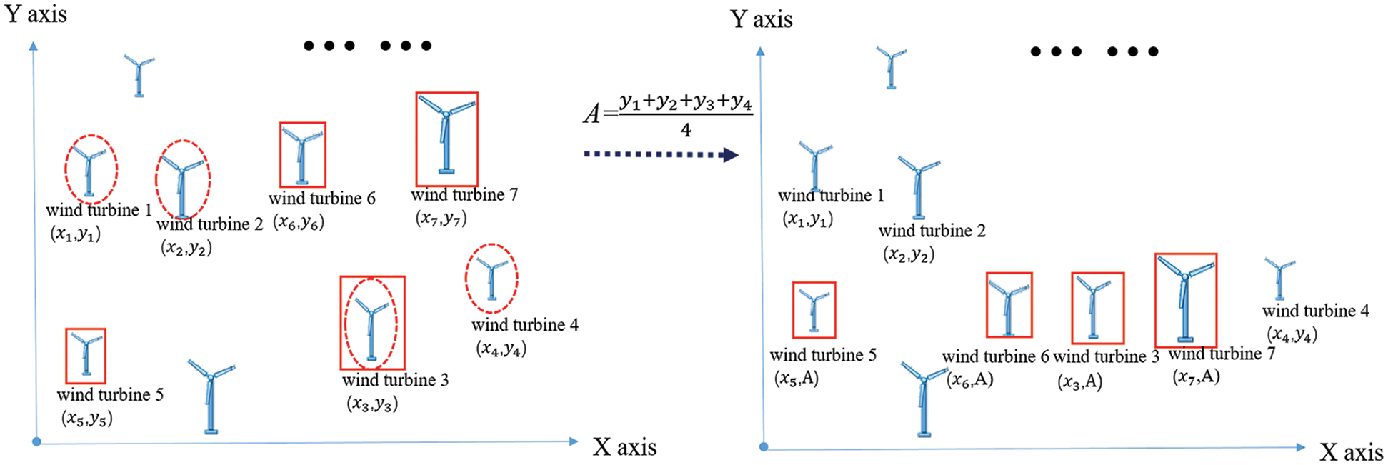
Figure 4: Strategy 4

Strategy 5: n3 wind turbines are randomly selected from wind farms, and the average x coordinates of these wind turbines are recorded as B . Then, select n4 wind turbines from the wind farm and set the x coordinates of these wind turbines to B .

Strategy 6: Randomly select n wind turbines and set them to random values.

Strategy 7: Randomly select Strategy 1 to Strategy 6 as Strategy 7.

These seven adjustment strategies can guide the algorithm to seek breakthroughs in different goals. To a certain extent, the algorithm not only has the global search ability, but also has a good local search ability.

2.5.2 Strategy Selection

In this paper, the roulette wheel algorithm is adopted to select the above seven strategies. The advantage of using this mechanism is that each strategy has the opportunity to be selected in each iteration, which increases the diversity of the position and the height of the wind turbine, so the algorithm has a good global search ability.

When the fitness value of population which selects si is less than the previous one, the corresponding selected probability λ(si) will be updated. The probability of being selected is calculated by (10)-(11):

Φ(si)=g(si)∑i=1Ng(si), (10)

λ(si)=1−Φ(si)∑iN(1−Φ(si)), (11)

where si refers to population i , g(si) is the fitness value of strategy i , Φ(si) is the weight of the fitness value, and λ(si) is the selected probability for this strategy.

3  Experimental Design and Results

3.1 Experimental Scheme Design

DEGM , DEEM and three-dimensional greedy algorithm are used to conduct experiments on fixed-hub height and multiple hub height in WOMH to verify that multiple hub heights can further improve the utilization of wind resources. In addition, the experiments also compare the performance of DEGM, DEEM and three-dimensional greedy algorithm in the above two models. DEEM refers to differential evolution with a new encoding mechanism. GREEDY is used instead of “three-dimensional greedy algorithm”. GREEDY is a classical mathematical probability algorithm, and DEEM is the latest and effective algorithm. So we chose these two algorithms to compare with DEGM. Finally, the probability of the emergence of seven adjustment strategies and the impact of these probabilities on the algorithm are analyzed.

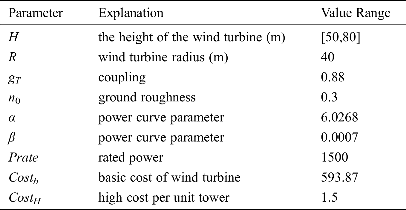
In order to ensure the rationality of the results, the experiments are conducted on different numbers of wind turbines in a wind scenario [4,15,23], and the scale of the wind farm is changed for each number of wind turbines. The specific parameters are shown in Tab. 1.

Table 1: Wind turbine parameters

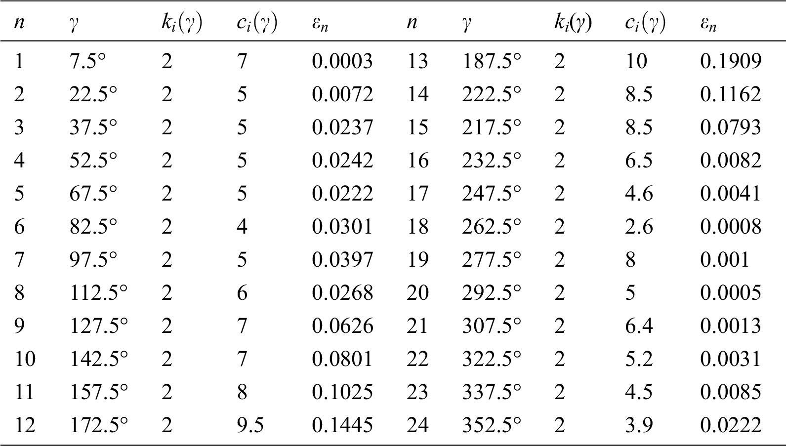
In order to simulate the real wind scenario, the following definition is adopted in this paper. The wind direction is defined as 0° from west to east, 90° from south to north, 180° from east to west and 270° from north to south. εn is the weight of each wind direction. ki(γ) is the shape parameter and ci(γ) is the scale parameter respectively. For details of εn , please see [11]. The specific parameters of the wind scenario are shown in Tab. 2.

Table 2: The specific parameters of the wind scenario

3.2 Experimental Results and Analysis

Tab. 3 records the LCOE obtained by GREEDY, DEEM and the DEGM. -F means the algorithm is applied to the wind farm with the fixed hub height, and -M means the algorithm is applied to a situation with multiple hub heights. In the experiment, both DEEM and the DEGM will be run 30 times. GREEDY is deterministic, so it only runs once.

In this kind of wind scenario, the distribution of the wind direction is very irregular. The probability distribution of the wind speed in each wind direction is also different, which puts higher requirements on the performance of the algorithm. In every case, the results of DEGM-M are smaller than those of DEEM-M and GREEDY-M.

Table 3: Comparison of the LCOE of the three algorithms when N is 5, 10, 20, 30 and 50, respectively

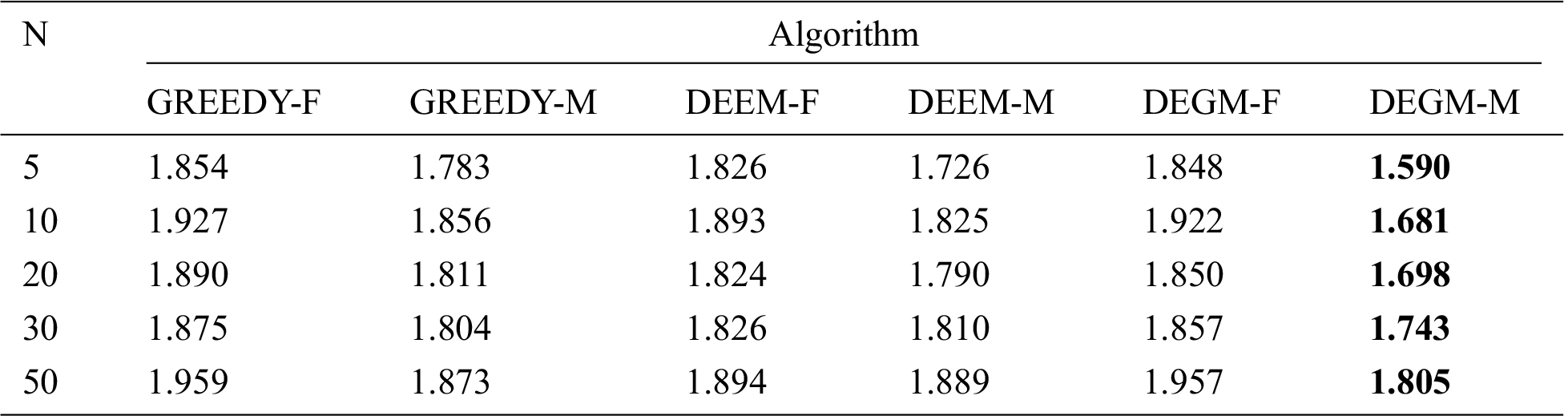
In the case of N = 5, 10, 20, 30, and 50, DEGM-M reduces the LCOE by 7.91%, 7.91%, 5.13%, 3.67%, and 4.45% compared with DEEM- M, respectively. Compared with GREEDY-M, DEGM-M was reduced by 10.81%, 9.43%, 6.88%, 3.38%, and 3.64%, respectively. This shows that the DEGM has a strong adaptability when facing complex wind scenes. In addition, no matter how the number of wind turbines varies, the performance of different algorithms in WOMH is always better than that of fixed hub height model. For example, when the number of wind turbines is 5, the LCOE of DEGM-M, DEEM-M and GREEDY-M are 13.96%, 5.48% and 3.83% lower than those of DEGM-F, DEEM-F and GREEDY-F, respectively. This shows that multiple hub heights are beneficial for reducing the influence of the wake effect.

Figs. 5 and 6 reflect the layout of wind turbines under different algorithms. Here we take the number of wind turbines as 5 and 50 as examples. The trend of DEGM arranging from low to high along a certain wind direction is obvious. The main reason the DEGM achieves an excellent performance in the complex wind scenario is that its seven adjustment strategies. These seven adjustment strategies constantly update the coordinates of wind turbines so that they are roughly arranged in lines. This layout further reduces the wake effect.

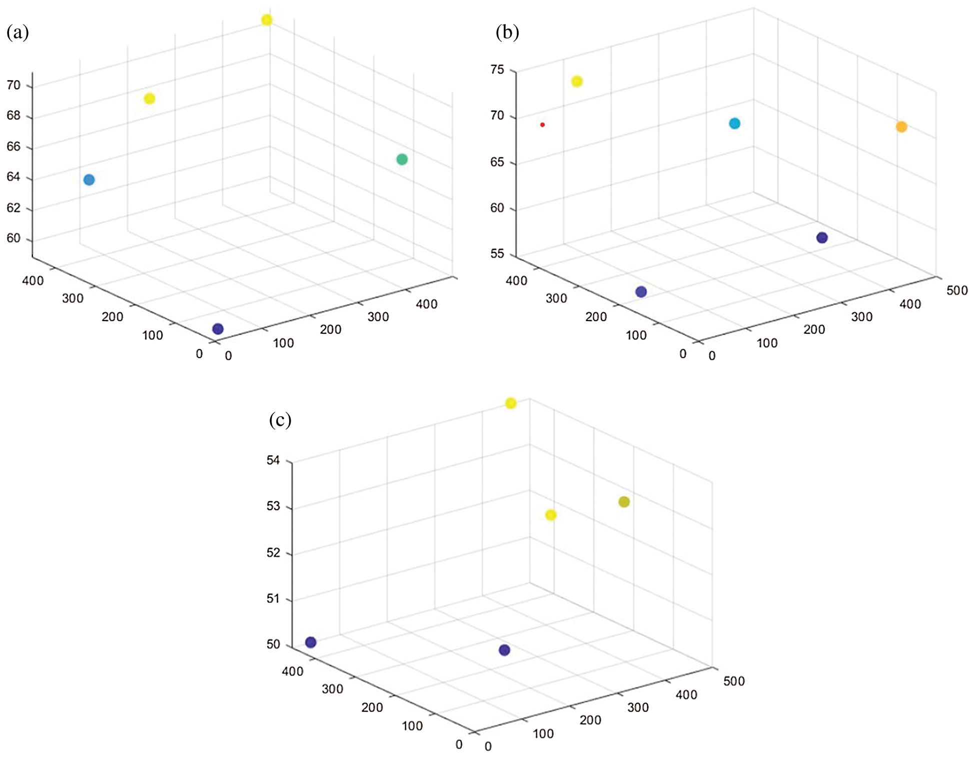
Figure 5: The layout of wind turbines under three algorithms when the number of wind turbines is 5 (a) The layout obtained by GREEDY-M (b) The layout obtained by DEEM-M (c) The layout obtained by DEGM-M

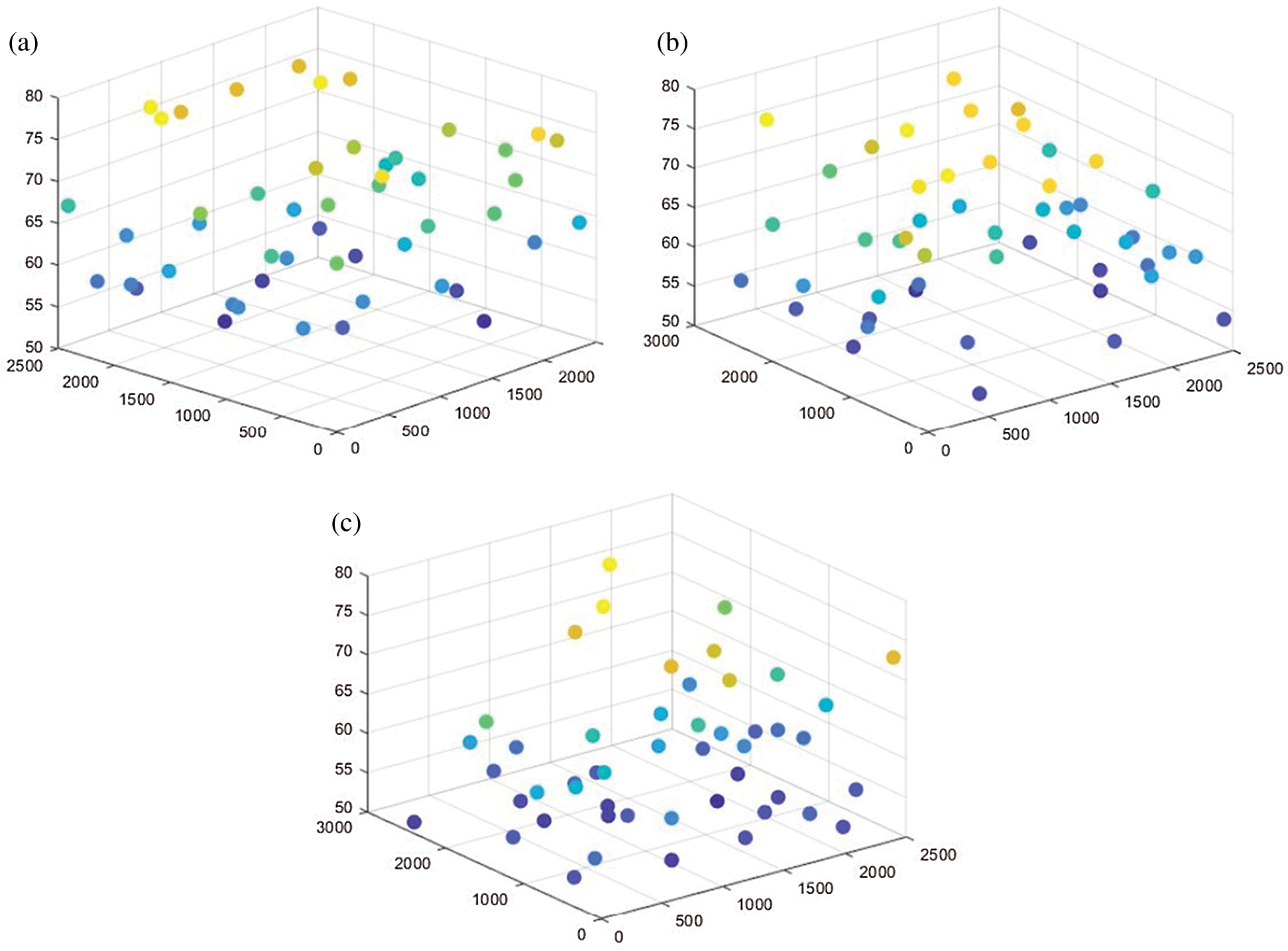
Figure 6: The layout of wind turbines under three algorithms when the number of wind turbines is 50 (a) The layout obtained by GREEDY-M (b) The layout obtained by DEEM-M (c) The layout obtained by DEGM-M

Fig. 7 records LCOE of three algorithms when FEs changes from 0 to 200000. From Fig. 7a, we can see that GREEDY is the most unsatisfactory in terms of the convergence speed and solution quality. Fig. 7b magnifies the results of DEEM and DEGM, and it shows that DEEM quickly converges to the a local optimal solution. In addition, it can also be observed in Fig. 7b that the curve of DEGM decreases significantly several times, which is not available in DEEM. Because the adjustment strategy of DEGM plays an important role, so that it will not converge to the local optimal solution prematurely.

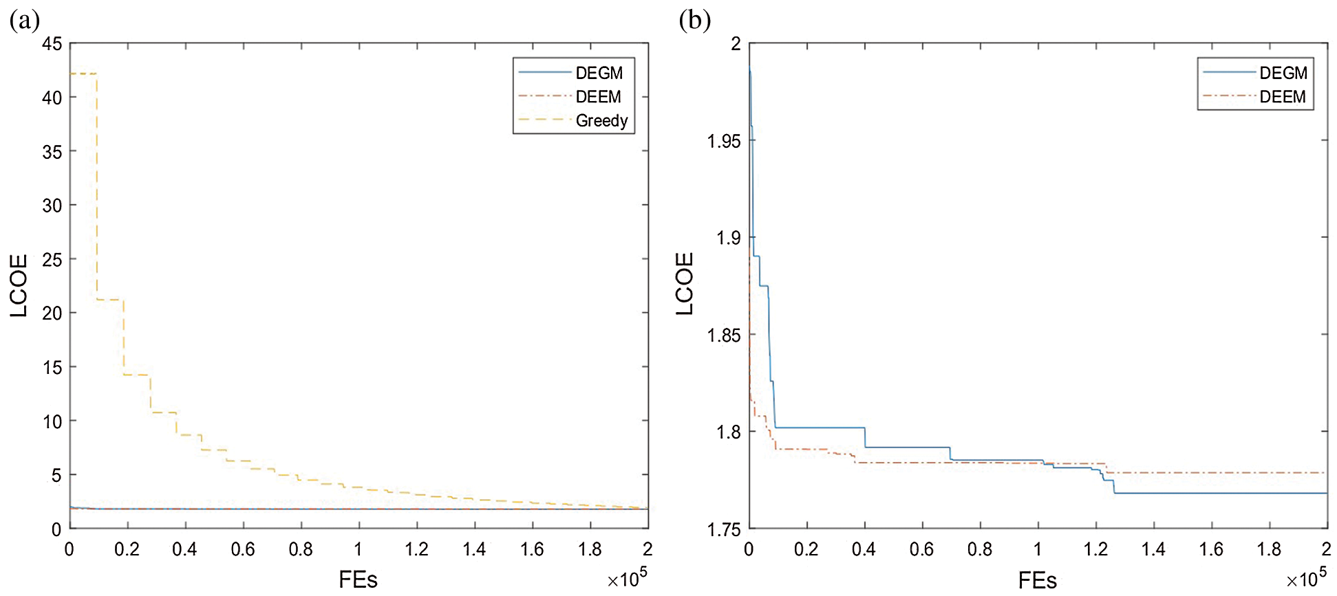
Figure 7: The LCOE convergence comparison among the three algorithms (a) The LCOE provided by DEEM, DEGM, GREEDY (b) The LCOE provided by the DEEM and DEGM

Fig. 8 records the relationship between strategy selected probability, selected strategy and FEs. From Fig. 8a, we can see that the probabilities of all strategies fluctuate obviously when FEs is less than 20000. When FEs is greater than 20000 and less than 40000, the probability of Strategy 1 and Strategy 6 decreases gradually, while the probability of other strategies increases. When FEs is greater than 40000, the probability of all strategies tends to be stable. In the end, the probability of Strategy 1 is the highest, and the probability of Strategy 6 is the lowest. It fully reflects that various strategies can show different performance in different periods of the algorithm, which reflects that the algorithm has a good adaptive ability. It is observed from Fig. 8b that although the probability of selecting different strategies varies, all kinds of strategies have the chance of being selected. Through Fig. 8a, we can find that the probability of strategy 6 being selected in the later stage is low, but from Fig. 8b we can see that it is still possible to be selected, which shows that the algorithm retains a certain diversity. To sum up, DEGM has good adaptive ability and maintains the diversity.

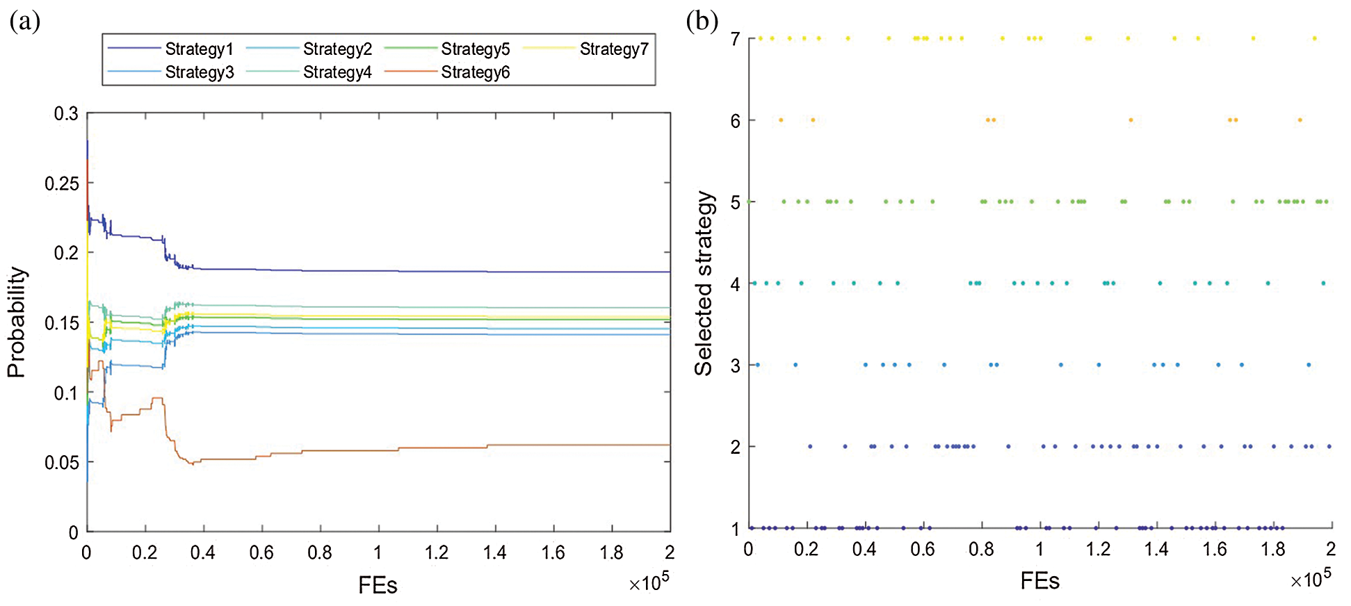
Figure 8: The relationship between strategies selected probability, selected strategy and FES (a) The relationship between selected probability of seven strategies and FEs (b) The selected strategy corresponding to FEs

4  Conclusions

A novel model called WOMH is proposed in this paper. Different from the traditional fixed hub height model, WOMH can effectively reduce the wake effect and achieve lower LCOE. In order to solve the WOMH, DEGM was proposed. In DEGM, the seven adjustment strategies are designed to update the coordinates of wind turbines and further reduce the Jensen wake effect between wind turbines. WOMH with DEGM provides a reference solution for the field of wind farm layout optimization. The wind farm layout optimization under the flexible multi-stage long-term planning optimization model of distributed multi-energy system will be further researched, which will comprehensively consider multiple dynamic factors, including energy demand, price.

Funding Statement: This paper was supported in part by Project funded by China Postdoctoral Science Foundation under Grant 2020M671552, in part by Jiangsu Planned Projects for Postdoctoral Research Funds under Grant 2019K223, in part by NUPTSF(NY220060), in part by the Opening Project of Jiangsu Key Laboratory of Data Science and Smart Software (No.2020DS301), in part by Natural Science Foundation of Jiangsu Province of China under Grant BK20191381, in part by the National Natural Science Foundation of China under Grant 61772286, Grant 61771258 and Grant 61876089.

Conflicts of Interest: The authors declare that they have no conflicts of interest to report regarding the present study.

References

 1.  M. Tan and Z. J. Zhang, “Wind turbine modeling with data-driven methods and radially uniform designs,” IEEE Transactions on Industrial Informatics, vol. 12, no. 3, pp. 1261–1269, 2016. [Google Scholar]

 2.  Y. S. Hamed, A. A. Aly, B. Saleh, A. F. Alogla, A. M. Aljuaid et al., “Vibration performance stability and energy transfer of wind turbine tower via pd controller,” Computers, Materials & Continua, vol. 64, no. 2, pp. 871–886, 2020. [Google Scholar]

 3.  R. Maheswari and R. Umamaheswari, “Wind turbine drivetrain expert fault detection system: Multivariate empirical mode decomposition based multi-sensor fusion with Bayesian learning classification,” Intelligent Automation & Soft Computing, vol. 26, no. 3, pp. 479–488, 2020. [Google Scholar]

 4.  G. Mosetti, C. Poloni and B. Diviacco, “Optimization of wind turbine positioning in large windfarms by means of a genetic algorithm,” Journal of Wind Engineering and Industrial Aerodynamics, vol. 51, no. 1, pp. 105–116, 1994. [Google Scholar]

 5.  A. Kusiak and Z. Song, “Design of wind farm layout for maximum wind energy capture,” Renewable Energy, vol. 35, no. 3, pp. 685–694, 2010. [Google Scholar]

 6.  F. Wang, D. Y. Liu and L. H. Zeng, “Study on computational grids in placement of wind turbines using genetic algorithm,” in 2009 World Non- Grid-Connected Wind Power and Energy Conference, IEEE, pp. 1–4, 2009. [Google Scholar]

 7.  R. Q. Sun, Z. H. He, L. Gao and J. L. Bai, “Station layout optimization genetic algorithm for four stations today location,” Journal of Physics: Conference Series, vol. 1176, pp. 062008, 2019. [Google Scholar]

 8.  J. W. Park, B. S. An, Y. S. Lee, H. Jung and I. Lee, “Wind farm layout optimization using genetic algorithm and its application to daegwallyeong wind farm,” JMST Advances, vol. 1, no. 4, pp. 249–257, 2019. [Google Scholar]

 9.  J. F. Cao, W. J. Zhu, W. Z. Shen and Z. Y. Sun, “Wind farm layout optimization with special attention on noise radiation,” Journal of Physics: Conference Series, vol. 1618, pp. 042022, 2020. [Google Scholar]

10. Y. Wu, S. Zhang, R. Q. Wang, Y. F. Wang and X. Feng, “A design methodology for wind farm layout considering cable routing and economic benefit based on genetic algorithm and GeoSteiner,” Renewable Energy, vol. 146, no. 3, pp. 687–698, 2020. [Google Scholar]

11. Y. Wang, H. Liu, H. Long, Z. Zhang and S. X. Yang, “Differential evolution with a new encoding mechanism for optimizing wind farm layout,” IEEE Transactions on Industrial Informatics, vol. 14, no. 3, pp. 1040–1054, 2018. [Google Scholar]

12. J. Herbert-Acero, J. Franco-Acevedo, M. Valenzuela-Rendón and O. Probst-Oleszewski, “Linear wind farm lay-out optimization through computational intelligence,” in Mexican Int. Conf. on Artificial Intelligence, Springer, pp. 692–703, 2009. [Google Scholar]

13. S. Chowdhury, J. Zhang, A. Messac and L. Castillo, “Optimizing the arrangement and the selection of turbines for wind farms subject to varying wind conditions,” Renewable Energy, vol. 52, no. 1–2, pp. 273–282, 2013. [Google Scholar]

14. H. Long, Z. J. Zhang, Z. Song and A. Kusiak, “Formulation and analysis of grid and coordinate models for planning wind farm layouts,” IEEE Access, vol. 5, pp. 1810–1819, 2017. [Google Scholar]

15. K. Chen, M. X. Song, X. G. Zhang and S. F. Wang, “Wind turbine layout optimization with multiple hub height wind turbines using greedy algorithm,” Renewable Energy, vol. 96, no. 1, pp. 676–686, 2016. [Google Scholar]

16. I. Katic, J. Hojstrup and N. O. Jensen, “A simple model for cluster efficiency,” European Wind Energy Association Conference and Exhibition, vol. 1, pp. 407–410, 1986. [Google Scholar]

17. Y. Chen, H. Li, K. Jin and Q. Song, “Wind farm layout optimization using genetic algorithm with different hub height wind turbines,” Energy Conversion and Management, vol. 70, no. 11–12, pp. 56–65, 2013. [Google Scholar]

18. N. Mohanapriya and B. Kalaavathi, “Adaptive image enhancement using hybrid particle swarm optimization and watershed segmentation,” Intelligent Automation and Soft Computing, vol. 25, no. 4, pp. 663–672, 2019. [Google Scholar]

19. H. Long and Z. J. Zhang, “A two-echelon wind farm layout planning model,” IEEE Transactions on Sustainable Energy, vol. 6, no. 3, pp. 863–871, 2015. [Google Scholar]

20. M. A. Lackner and C. N. Elkinton, “An analytical framework for offshore wind farm layout optimization,” Wind Engineering, vol. 31, no. 1, pp. 17–31, 2016. [Google Scholar]

21. J. S. González, M. B. Payán, J. M. R. Santos and F. G. Longatt, “A review and recent developments in the optimal wind-turbine micro-siting problem,” Renewable and Sustainable Energy Reviews, vol. 30, pp. 133–144, 2014. [Google Scholar]

22. Y. Xue, T. Tang, W. Pang and A. X. Liu, “Self-adaptive parameter and strategy based particle swarm optimization for large-scale feature selection problems with multiple classifiers,” Applied Soft Computing, vol. 88, no. 4, pp. 106031, 2020. [Google Scholar]

23. L. H. Zhu, Z. Q. Wu, L. Wang and Y. Wang, “The identification of the wind parameters based on the interactive multi-models,” Computers, Materials & Continua, vol. 65, no. 1, pp. 405–418, 2020. [Google Scholar]

This work is licensed under a Creative Commons Attribution 4.0 International License, which permits unrestricted use, distribution, and reproduction in any medium, provided the original work is properly cited.