DOI:10.32604/iasc.2021.016219
| Intelligent Automation & Soft Computing DOI:10.32604/iasc.2021.016219 | |
| Article |
A Deep Learning Approach for the Mobile-Robot Motion Control System
1King Saud University, Riyadh, 11451, Saudi Arabia
2King Abdulaziz City for Science and Technology, Riyadh, Saudi Arabia
3College of Computing and Information Technology, University of Bisha, Bisha, 67714, Saudi Arabia
4Laboratory for Analysis, Conception and Control of Systems, LR-11-ES20, Department of Electrical Engineering, National Engineering School of Tunis, Tunis El Manar University, Tunis, 1002, Tunisia
*Corresponding Author: Rihem Farkh. Email: rfarkh@ksu.edu.sa
Received: 22 December 2020; Accepted: 24 January 2021
Abstract: A line follower robot is an autonomous intelligent system that can detect and follow a line drawn on floor. Line follower robots need to adapt accurately, quickly, efficiently, and inexpensively to changing operating conditions. This study proposes a deep learning controller for line follower mobile robots using complex decision-making strategies. An Arduino embedded platform is used to implement the controller. A multilayered feedforward network with a backpropagation training algorithm is employed. The network is trained offline using Keras and implemented on a ATmega32 microcontroller. The experimental results show that it has a good control effect and can extend its application.
Keywords: Neural control system; real-time implementation; navigation environment; and mobile robots
With the advancement of technology and science and improvement of productivity, robots are increasingly being used in various fields ranging from industry, military, healthcare and related fields [1], search and rescue, management, and agriculture, allowing humans to accomplish complicated tasks [2,3]. Currently, robots are developing in the direction of high precision, high speed, and stable safety [4]. To design and manufacture useful products, intelligent mobile robots combine control, electronic, computer, software, and mechanical engineering [5].
Mobile robots can move between locations to perform desired and complex tasks [6]. A mobile robot is controlled by software and integrated sensors, such as infrared, ultrasonic, and magnetic sensors, and webcams and GPSs. Wheels and DC motors are used to drive the robot [7].
Line follower robots can be utilized in many industrial applications, such as transporting heavy materials and materials that pose a danger to human safely, e.g., nuclear products. These robots are also capable of monitoring patients in hospitals and notifying medical personnel of dangerous conditions [8]. A significant number of researchers have focused on control techniques and smart vehicle navigation, since traditional tracking techniques are limited owing to environmental instability under which a vehicle is intended to move. Therefore, intelligent control mechanisms, such as neural networks, are required. Such mechanisms provide a good solution vehicle navigation problems owing to their ability to learn the nonlinear relationship between input and sensor values [9].
Deep learning technology has significantly advanced developments in artificial intelligence, particularly in the fields of image processing, object recognition, detection, computer vision, and mobile-robot control [10–13].
Deep learning is a branch of artificial intelligence used to solve various problems, particularly in logic and rule-based systems [14]. Deep learning has helped researchers develop breakthrough methods related to the perception capabilities of robotic systems. These methods empower robots to learn from sensory data and, based on learned models, to react and take decisions accordingly [15]. Recent advances in human-robot interaction, complex robotic tasks, intelligent reasoning, and decision-making are, to some extent, the result of the evolution and success of deep learning algorithms [16]. Using deep learning techniques, the ability of an intelligent robot to navigate and recognize a given place in a complex environment was improved and approached human level capability [17].
Several attempts have been made to improve low-cost autonomous cars using different neural network configurations. Kaiser et al. [18] used a multilayered perceptron network for mobile-robot motion planning. The network was implemented on a PC with an Intel Pentium 350 MHz processor. In [19], the problem of mobile-robot navigation was solved with the aid of a local neural network model.
In this study, low-cost implementation of a multilayered feedforward network with a backpropagation training algorithm suitable for a line follower robot is realized using the Arduino platform.
2 Line Follower Robot Architecture
In this section, the architecture, engine capabilities, sensor system housing of the brain neural network, system block diagram, and the design and implementation of the neural network are described. First, a suitable configuration is selected to develop a line follower robot using three infrared sensors connected through the Arduino Uno to the motor driver IC. This configuration is illustrated in the block diagram shown in Fig. 1.
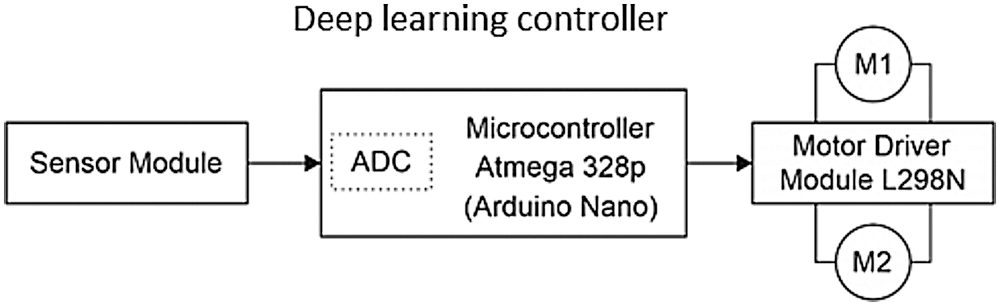
Figure 1: Block diagram of the line follower robot
Implementing the system on the Arduino Uno ensures the following:
• moving the robot in the desired direction
• reading the infrared sensors for line detection
• predicting the direction using the deep learning controller
• controlling the four DC motors and determining the speed of the left and the right motors
The path line is shown in Fig. 2.
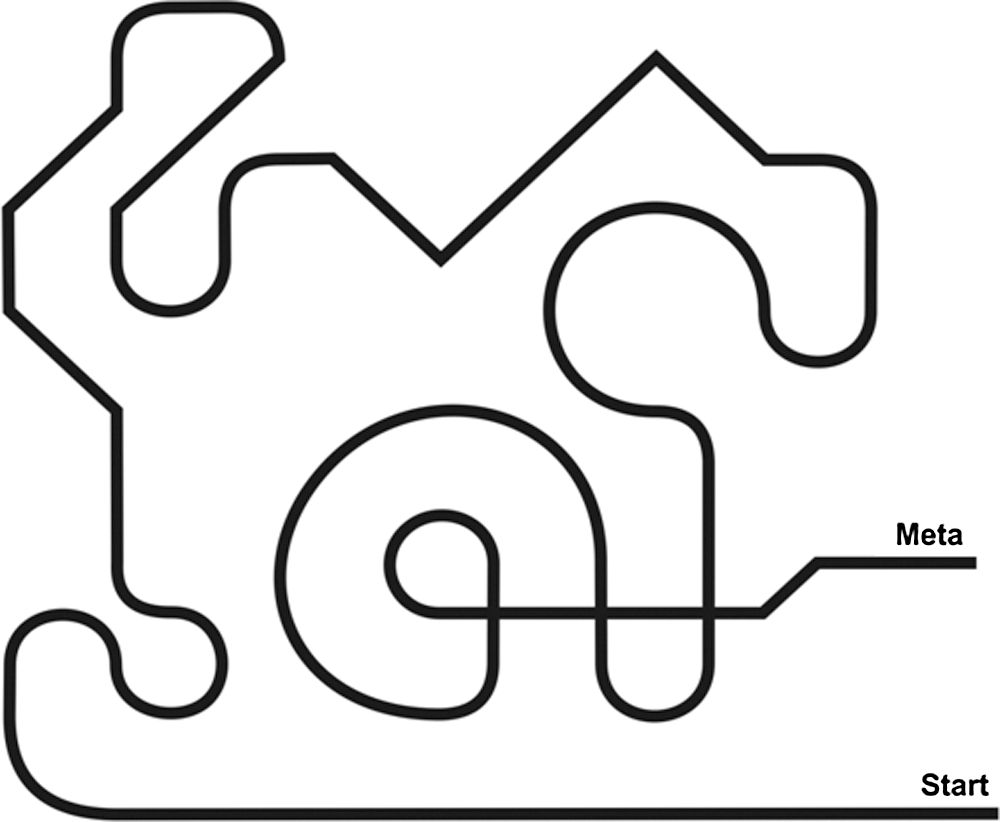
Figure 2: Robot’s path line
In this study, the proposed mobile-robot design can be easily modified and adapted to new and future research studies. The physical appearance of the robot was evaluated, and its design was based on several criteria, such as functionality, material availability, and mobility. During the analysis of different guided robots of reduced size and simple structure.
The following parts were used in the robot’s construction:
1. Four wheels
2. Four DC motors
3. Two base structures
4. Control board formed using the Arduino ATmega 32 board
5. L298 IC circuit for DC-motor driving
6. Expansion board
7. Line tracking module
2.2 Arduino Uno Microcontroller
The Arduino Uno is a microcontroller board based on the ATmega328P (Fig. 3). It has 14 digital input/output pins (six of which can be used as PWM outputs), six analog inputs, a 16-MHz quartz crystal, a USB connection, a power jack, an ICSP header, and a reset button. It contains everything needed to support the microcontroller and can be simply connected to a computer with a USB cable. It can be powered by an AC-to-DC adapter or a battery [20]. In this study, the Arduino microcontroller is very well suited to drive a PWM signal for the DC motor. The microcontroller is capable of improving the output response of the DC motor position control system.
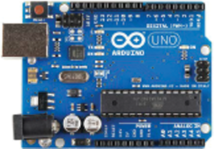
Figure 3: Arduino Uno
The line tracking sensor used is capable of detecting white lines on a black surface and black lines on a white surface (Fig. 4). The single line tracking signal provides a stable output TTL signal for more accurate and stable line tracking. A multichannel operation can be easily achieved by installing the required line tracking robot sensors [21].
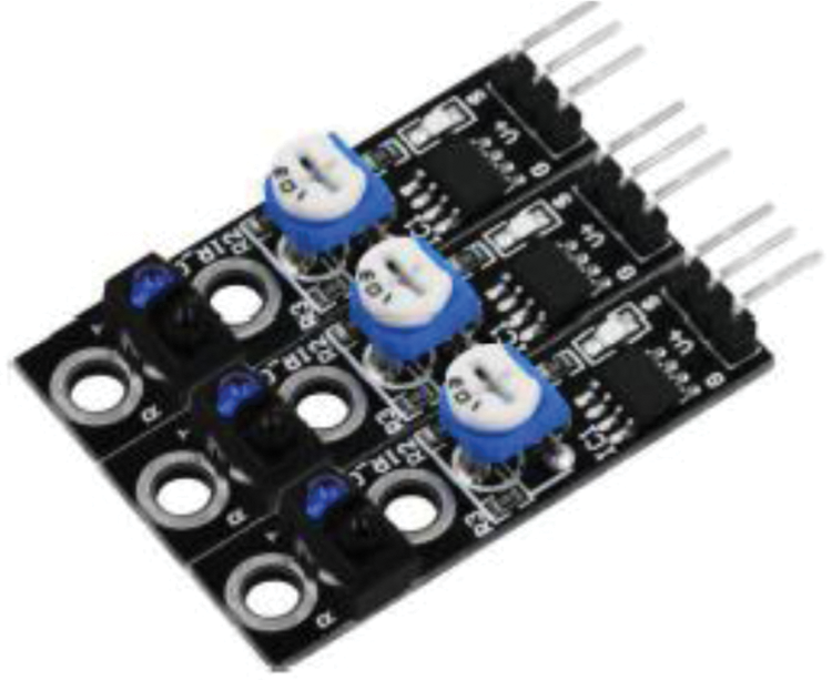
Figure 4: Tracking sensor
The L298N motor driver (Fig. 5) comprises two complete H-bridge circuits; thus, it can drive a pair of DC motors. This feature makes it ideal for robotic applications because most robots have two or four powered wheels operating at 5- and 35-V DC with a peak current of up to 2 A. This module incorporates two screw terminal blocks for Motors A and B, and another screw terminal block for the ground pin, the VCC for the motor, and a 5-V pin, which can either be an input or output. The pin assignments for the L298N dual H-bridge module are shown in Tab. 1. The digital pin, assigned from HIGH to LOW or LOW to HIGH, is used for IN1 and IN2 on the L298N board to control the direction. The controller output PWM signal is sent to the ENA or ENB to control the position. The forward and reverse speed or position control of the motor is realized using the PWM signal [21]. Then, using the Arduino analogWrite() function, the PWM signal is sent to the Enable pin of the L298N board, which drives the motor.
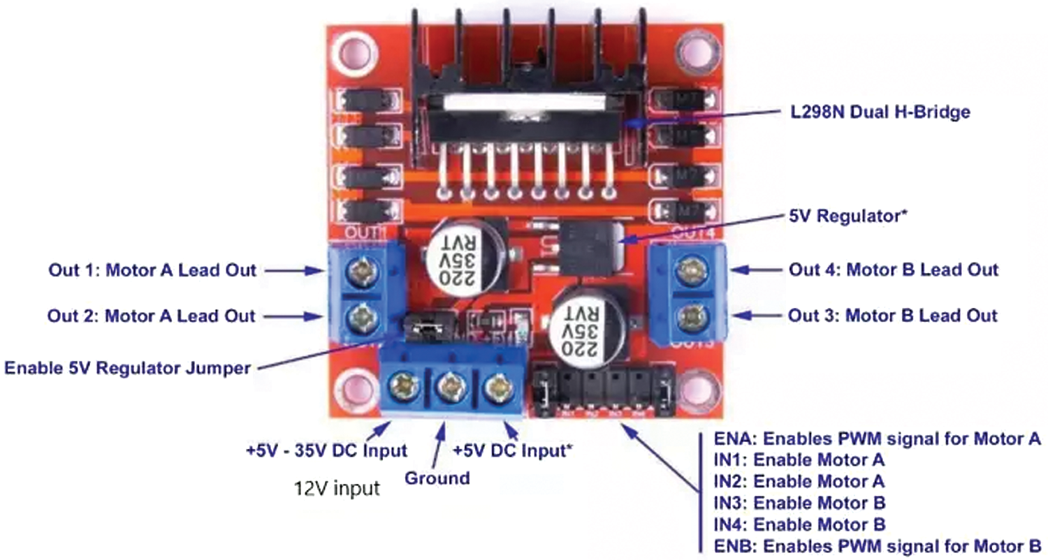
Figure 5: LN298 IC motor driver
A diagram showing the wire connections used for the design and implementation of the mobile robot is given in Fig. 6, including the embedded system, line tracking sensors, DC motors, and L298 IC circuit for driving the motors.
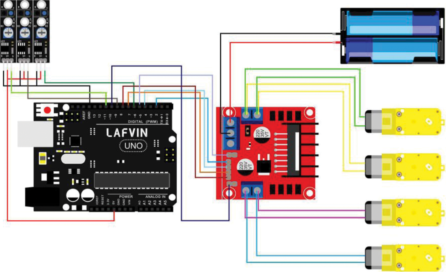
Figure 6: Wire connections
3 Neural Network Controller for Line Follower Robot
A neural network is used to develop the robot control navigation. Here, the neural network predicts the robot’s position on the path and provides a control signal to the IC driver for motion control (Fig. 7). The neural network, i.e., a multilayered perceptron (MLP), demonstrates good characteristics relative to solving classification problems that are similar to this study’s target problem. In addition, it is a relatively simple architecture for implementation in a robot.
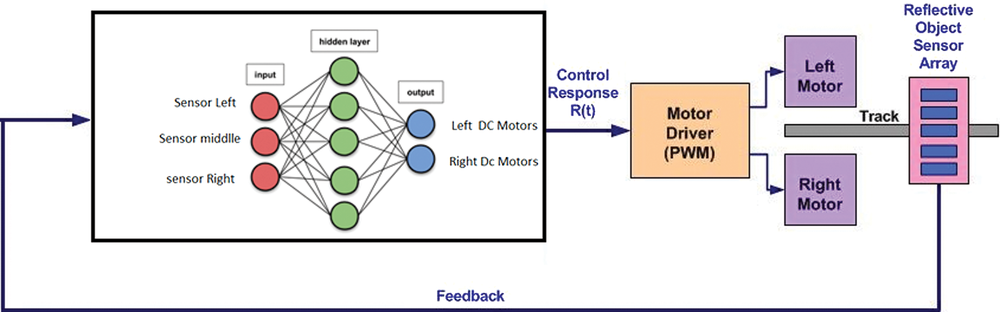
Figure 7: Mobile robot motion control system
3.1 Artificial Neural Network Mathematical Model
An artificial neural network (ANN) comprises many simple but highly interconnected processing elements, and these elements are processed by variations in external inputs. The presented ANN structure was constructed using multiple weighted hidden layers, which are supervised by a feedforward network using a backpropagation algorithm, which is a widely used method in many applications [22].
ANNs are best suited to human-like operations, e.g., image processing, speech recognition, robotic control, and the power sector for power system protection and control management. ANNs can be compared to the human brain. The human brain operates quickly and comprises many neurons (or nodes). Each signal or bit of information travels through a neuron, where it is processed, calculated, manipulated, and then transferred to the next neuron cell. The overall processing speed of each neuron or node may be slow; however, the overall network is very fast and efficient.
3.2 Artificial Neural Network Structure
The first layer used in the ANN is the input layer and the highest layer, i.e., the output layer. Each bit of information is processed through a single layer, i.e., hidden layers (intermediate layer) and output layers. The signal or data are manipulated, calculated, and processed in each layer, and then transferred to the respective network layers. Information is processed through layers or nodes in an ANN network; thus, more efficient results can be achieved as the number of hidden layers increases.
The ANN operates through these layers and calculates and overwrites the results as it is trained using given data. Thus, the entire network is quite efficient, can predict future outcomes, and make necessary decisions. This is why ANNs are frequently compared to the neuron cells of the human brain.
The neural network developed in this study comprises three inputs or neurons. The first input is dedicated to the left sensor, the second is dedicated to the middle sensor, and the third is dedicated to the right sensor. Note that the hidden layer comprises 10 neurons. Then, the output layer is formed of two neurons for the left and right motors (Fig. 8).
In this network, n (=3) is the number of inputs, H (=10) is the number of hidden cells, and T (=2) is the number of output layers. The weight between an input unit i and hidden unit j is denoted W1i, j, and the weight between a hidden unit i and output unit j is denoted W2i,j. In addition, the hidden and output layers employ a sigmoid function as the activation function.
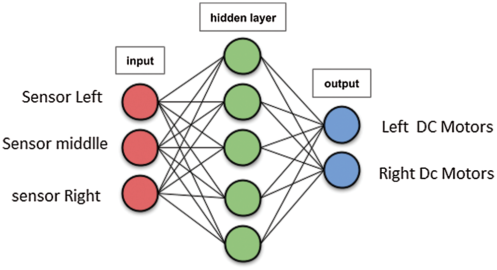
Figure 8: Neural network structure
Here, two-layered feedforward networks supervised by the backpropagation algorithm are employed. Thus, two functions must be constructed, i.e., one for the inputs to hidden layers, and the other for the hidden layers to output layers or targets. A block diagram showing the equations of the final output is shown in Fig. 9.
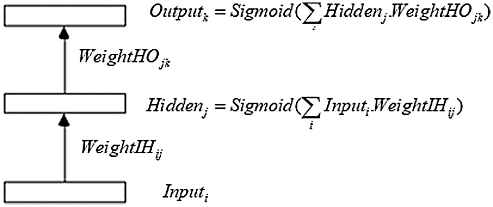
Figure 9: Neural network equations
4 Neural Network Controller Implementation
The neural network algorithm developed and implemented for the proposed mobile robot was programmed in the C language for implementation in an embedded system. However, there are some challenges associated with implementing a neural network in a very small system, and these challenges have been significant for the inexpensive microcontrollers and hobbyist boards of earlier generations. Fortunately, Arduinos, like many modern boards, can complete the required tasks quickly.
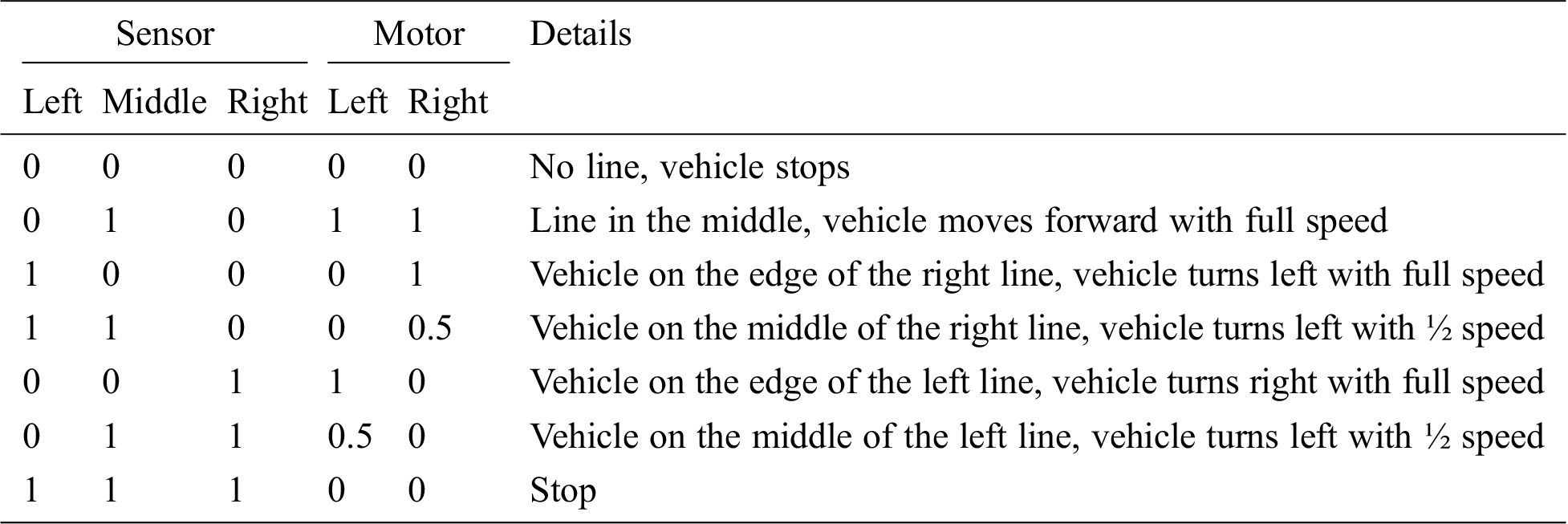
The Arduino Uno used in this study is based on Atmel’s ATmega328 microcontroller, and its 2 K of SRAM is adequate for a sample network with three inputs, 10 hidden cells, and two outputs. By exploiting the Arduino’s GCC language support for multidimensional arrays and floating point math, the programming process becomes very manageable. The neural network architecture and algorithm design apprenticeship are monitored offline by Keras, where the values of synaptic weights extract the entailment. Here Keras was used to train the proposed ANN according to the following sensor positions on the path line. The sensor positions are shown in Fig. 10 and indicated in Tab. 1.
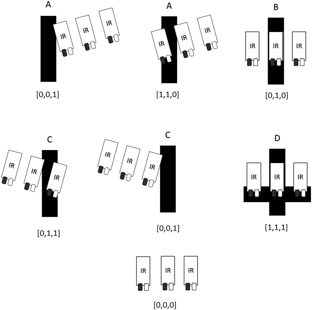
Figure 10: Sensor positions
Tab. 1 shows the manual training data for our neural network.
Table 1: Follower-logic target/neuronal network manual training data
After running 1000 iterations with a decaying learning rate, the weight of each dense was found with RMS = 0.08%. Here, the weights connecting the input layer to the hidden layer are stored in a dense_1 matrix with three rows and 10 columns.
dense_1
• [−1.6969934, −3.46079, 4.466045, −3.3381639, 2.7561083, 2.5783126, −5.0599, 1.770869, −0.8076482, −3.3734348],
• [ 2.807798, −2.7026825, 1.7920414, −5.039168, −1.7310187, 5.8257327, −2.5614583, −2.3312418, −4.9812517, 0.24215572],
• [ 4.393107, 1.4633285, −2.6768272, −1.2254419, −4.0297103, 2.8168633, 2.6069236, −4.016101, −3.3138442, 3.4869163]
In addition, the weights connecting the hidden layer to the output are stored in a dense_2 matrix with 10 rows and two columns.
dense_2
• [3.4826534, 0.99970883],
• [−2.990506, −4.2969046],
• [−2.000733, 4.053016],
• [−6.710817, −7.727256],
• [−3.4904156, 4.05857],
• [3.1300664, 3.464316],
• [0.44800535, −4.182376],
• [−3.768459, −0.8049714],
• [−7.593585, −7.1745195],
• [ 5.2892675, −2.603934]
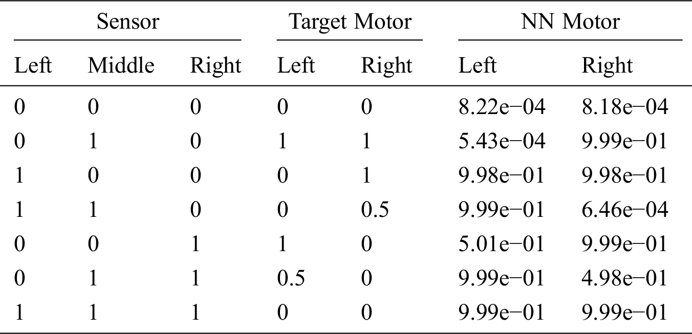
A comparison between real targets and the predictions calculated by Keras is given in Tab. 2.
Table 2: Comparison of real targets and neural network predictions
A single neuron receives an input (In) and produces an output activation (Out), and the activation function calculates the neuron’s output based on the sum of the weighted connections feeding that neuron. The most common activation function, i.e., the sigmoid function, is expressed as follows.
Out = 1.0/(1.0 + exp(-In))
The following C code is used to compute the hidden unit activation.
/* j loop computes hidden unit activations */
for(j = 1; j <= NumHidden; j++)
{
SumH[j]=WeightIH [0][j]; for(i = 1; i <= NumInput; i++) {
SumH[j] += Input[i] * WeightIH[i][j];
} Hidden[j] = 1.0/(1.0 + exp(-SumH[j]));
}
We use the following C code to compute the output unit activation:
/* k loop computes output unit activations */
for(k = 1; k <= NumOutput; k++)
{
SumO[k]=WeightHO [0][k]; for(j = 1; j <= NumHidden; j++) {
SumO[k] += Hidden[j] * WeightHO[j][k];
} Output[k] = 1.0/(1.0 + exp(-SumO[k]));
}
4.2 Neural Network Implementation Using Python and Keras
The neural network architecture and algorithm design apprenticeship are monitored offline by Keras, where the values of synaptic weights extract the entailment.
Keras is a powerful and easy-to-use Python library for developing and evaluating deep learning models. It wraps around the efficient numerical computation libraries Theano and TensorFlow, and this allows users to define and train neural network models using only a few short lines of code.
1. A random number generator is initialized with a fixed seed value; thus, the same code can be run repeatedly, and the same result is obtained.
from keras.models import Sequential
from keras.layers import Dense
import numpy
numpy.random.seed(7)
2. The models in Keras are defined as a sequence of layers. A fully-connected network structure with three layers is used, and the fully-connected layers are defined using the Dense class. The first layer is created with the input_dim argument by setting it to 3 for the three input variables. The number of neurons in the layer can be specified as the first argument, and the activation function can be specified using the activation argument. Note that the sigmoid activation function is used for all layers. The hidden layer has 10 neurons and expects three input variables (e.g., input_dim=3). Finally, the output layer has two neurons to predict the class.
model = Sequential()
model.add(Dense(10, input_dim = 3,activation = ‘sigmoid’,use_bias = False))
model.add(Dense(2, activation = ‘sigmoid’,use_bias = False))
3. Once the model is defined, it can be compiled. Here, the loss function must be specified to evaluate a set of weights, and an optimizer is used to search through different weights in the network. The mse loss and rmsprop algorithms are used for our target case.
# Compile model
model.compile(loss = ‘mse’, optimizer = ‘RMSprop’, metrics = [rmse])
4. The proposed model can be trained or fit to the loaded data by calling the fit() function. The training process runs for a fixed number of iterations through a dataset called epochs. Here, the batch size is the number of instances evaluated before performing a weight update in the network via trial and error.
# Fit the model
model.fit(X, Y, epochs = 10000, batch_size = 10)
5. The proposed neural network was trained on the entire dataset, and the network performance was obtained for the same dataset.
# Evaluate the model
scores = model.evaluate(X, Y)
The complete code is given as follows.
from keras.models import Sequential
from keras.layers import Dense
import numpy
from keras import backend
# from sklearn.model_selection import train_test_split
#from matplotlib import pyplot
# fix random seed for reproducibility
numpy.random.seed(7)
def rmse(y_true, y_pred):
return backend.sqrt(backend.mean(backend.square(y_pred - y_true), axis = −1))
# # split into input (X) and output (Y) variables
X = numpy.loadtxt(‘input_31.csv’, delimiter = ‘,’)
Y = numpy.loadtxt(‘output_31.csv’, delimiter = ‘,’)
#(trainX, testX, trainY, testY) = train_test_split(X, Y, test_size = 0.25, random_state = 6)
# create model
model = Sequential()
model.add(Dense(10, input_dim = 3, activation = ‘sigmoid’,use_bias = False))
model.add(Dense(2, activation = ‘sigmoid’,use_bias = False))
# Compile model
model.compile(loss = ‘mse’, optimizer = ‘RMSprop’, metrics = [rmse])
# Fit the model
model.fit(X, Y, epochs = 10000)
# evaluate the model
#result = model.predict(testX)
#print(result- testY)
scores = model.evaluate(X, Y)
The vehicle with the trained neural network controller was successfully tested on various paths. Note that its speed must be variable to cope with real situations. The neural controller can be further refined by adding speed input such so that the robot can move faster in a straight path and reduce its speed in curves.
In this study, we have proposed a mobile-robot platform with a fixed four-wheel configuration chassis and an electronic system designed using Arduino Uno interfaces. The results demonstrate that neural networks are well suited to mobile robots because they can operate with imprecise information. More advanced and intelligent control methods based on computer vision and convolutional neural networks can be developed and implemented using a Raspberry Pi, which is more powerful than any Arduino board.
Acknowledgement: The authors acknowledge the support of King Abdulaziz City of Science and Technology.
Funding Statement: The authors received no specific funding for this study.
Conflicts of Interest: The authors declare that they have no conflicts of interest to report regarding the present study.
1. K. Chakraborty, S. Bhatia, S. Bhattacharyya, J. Platos, R. Bag et al., “Sentiment analysis of COVID-19 tweets by deep learning classifiers—a study to show how popularity is affecting accuracy in social media,” Applied Soft Computing, vol. 97, pp. 106754, 2020. [Google Scholar]
2. H. Masuzawa, J. Miura and S. Oishi, “Development of a mobile robot for harvest support in greenhouse horticulture-Person following and mapping,” in International Symposium on System Integration, Taipei, pp. 541–546, 2017. [Google Scholar]
3. Z. Zhang, P. Li, S. Zhao, Z. Lv, F. Du et al., “Du etal, An adaptive vision navigation algorithm in agricultural IoT system for smart agricultural robots,” Computers, Materials & Continua, vol. 66, no. 1, pp. 1043–1056, 2021. [Google Scholar]
4. L. Juang and S. Zhang, “Intelligent service robot vision control using embedded system,” Intelligent Automation and Soft Computing, vol. 25, no. 3, pp. 451–458, 2019. [Google Scholar]
5. T. Jumphoo, M. Uthansakul, P. Duangmanee, N. Khan and P. Uthansakul, “Soft robotic glove controlling using brainwave detection for continuous rehabilitation at home,” Computers, Materials & Continua, vol. 66, no. 1, pp. 961–976, 2021. [Google Scholar]
6. R. Siegwart and I. R. Nourbakhsh. Introduction to Autonomous Mobile Robots. A Bradford Book, The MIT Press, London, England, pp. 12–22, 2011. [Google Scholar]
7. S. E. Oltean, “Mobile robot platform with arduino uno and raspberry pi for autonomous navigation,” Procedia Manufacturing, vol. 32, no. 1, pp. 572–577, 2019. [Google Scholar]
8. D. Janglova, “Neural networks in mobile robot motion,” International Journal of Advanced Robotic Systems, vol. 1, no. 3, pp. 15–22, 2004. [Google Scholar]
9. F. Li, J. Zhang, E. Szczerbicki, J. Song, R. Li et al., “Deep learning-based intrusion system for vehicular ad hoc networks,” Computers, Materials & Continua, vol. 65, no. 1, pp. 653–681, 2020. [Google Scholar]
10. Y. Tian, L. Wang, H. Gu and L. Fan, “Image and feature space-based domain adaptation for vehicle detection,” Computers, Materials & Continua, vol. 65, no. 3, pp. 2397–2412, 2020. [Google Scholar]
11. R. Yin and J. Yang, “Research on robot control technology based on vision localization,” Journal on Artificial Intelligence, vol. 1, no. 1, pp. 37–44, 2019. [Google Scholar]
12. H. Wu, Q. Liu and X. Liu, “A review on deep learning approaches to image classification and object segmentation,” Computers, Materials & Continua, vol. 60, no. 2, pp. 575–597, 2019. [Google Scholar]
13. M. A. Khan, A. Rehman, K. M. Khan, M. A. Al Ghamdi and S. H. Almotiri, “Enhance intrusion detection in computer networks based on deep extreme learning machine,” Computers, Materials & Continua, vol. 66, no. 1, pp. 467–480, 2021. [Google Scholar]
14. J. Shabbir and T. Anwer, “A survey of deep learning techniques for mobile robot applications,” arXiv preprint arXiv:1803.07608, 2018. [Google Scholar]
15. P. Yang, K. Sasaki, K. Suzuki, K. Kase, S. Sugano and T. Ogata, “Repeatable folding task by humanoid robot worker using deep learning,” IEEE Robotics and Automation Letters, vol. 2, no. 2, pp. 397–403, 2017. [Google Scholar]
16. R. L. Truby, C. D. Santina and D. Rus, “Distributed proprioception of 3D configuration in soft, sensorized robots via deep learning,” IEEE Robotics and Automation Letters, vol. 5, no. 2, pp. 3299–3306, 2020. [Google Scholar]
17. H. Li, Q. Zhang and D. Zhao, “Deep reinforcement learning-based automatic exploration for navigation in unknown environment,” IEEE Transactions on Neural Networks and Learning Systems, vol. 31, no. 6, pp. 2064–2076, 2020. [Google Scholar]
18. F. Kaiser, S. Islam, W. Imran, K. H. Khan and K. M. A. Islam, “Line-follower robot: Fabrication and accuracy measurement by data acquisition,” in International Conference on Electrical Engineering and Information & Communication Technology, Dhaka, pp. 1–6, 2014. [Google Scholar]
19. H. A. Awad and M. A. Al-Zorkany, “Mobile robot navigation using local model networks,” International Journal of Information Technology, vol. 1, no. 2, pp. 58–63, 2004. [Google Scholar]
20. P. Gaimar, The Arduino Robot: Robotics for Everyone. Kindle Edition, pp. 100–110, 2020. [Online]. Available: https://www.amazon.com/Arduino-Robot-Robotics-everyone-ebook/dp/B088NPQQG9. [Google Scholar]
21. S. F. Barrett, Arduino II: systems, Synthesis Lectures on Digital Circuits and Systems, pp. 10–20, 2020. [Google Scholar]
22. V. Silaparasetty, Deep Learning Projects Using TensorFlow 2: Neural Network Development with Python and Keras. Apress, pp. 10–22, 2020. [Google Scholar]
 | This work is licensed under a Creative Commons Attribution 4.0 International License, which permits unrestricted use, distribution, and reproduction in any medium, provided the original work is properly cited. |