DOI:10.32604/iasc.2021.017890
| Intelligent Automation & Soft Computing DOI:10.32604/iasc.2021.017890 | |
| Article |
Inference of Truncated Lomax Inverse Lomax Distribution with Applications
1Department of Mathematics, Faculty of Science, Jazan University, Jazan, Saudi Arabia
2Faculty of Graduate Studies for Statistical Research, Cairo University, Giza, 12613, Egypt
3The Higher Institute of Commercial Sciences, Al Mahalla Al Kubra, 31951, Egypt
4Deanship of Information Technology, King Abdulaziz University, Jeddah, 21589, Kingdom of Saudi Arabia
5Department of Mathematics, Faculty of Science, Jazan University, Jazan, Saudi Arabia
6Faculty of Business Administration, Sinai University, Cairo, Egypt
*Corresponding Author: M. Elgarhy. Email: m_elgarhy85@sva.edu.eg
Received: 12 February 2021; Accepted: 16 March 2021
Abstract: This paper introduces a modified form of the inverse Lomax distribution which offers more flexibility for modeling lifetime data. The new three-parameter model is provided as a member of the truncated Lomax-G procedure. The new modified distribution is called the truncated Lomax inverse Lomax distribution. The density of the new model can be represented as a linear combination of the inverse Lomax distribution. Expansions for quantile function, moment generating function, probability weighted moments, ordinary moments, incomplete moments, inverse moments, conditional moments, and Rényi entropy measure are investigated. The new distribution is capable of monotonically increasing, decreasing, reversed J-shaped and upside-down shaped hazard rates. Maximum likelihood estimators of the population parameters are derived. Also, the approximate confidence interval of parameters is constructed. A simulation study framework is established to assess the accuracy of estimates through some measures. Simulation outcomes show that there is a great agreement between theoretical and empirical studies. The applicability of the truncated Lomax inverse Lomax model is illustrated through two real lifetime data sets and its goodness-of-fit is compared with that of the recent models. In fact, it provides a better fit to these data than the other competitive models.
Keywords: Truncated Lomax-G family; inverse Lomax distribution; maximum likelihood method; moments
The inverse Lomax (IL) distribution is very flexible in analyzing situations of different types of hazard rate function. It is a member of the inverted family of distributions, that is, the IL distribution is the reciprocal of the well-known Lomax distribution. Kleiber et al. [1] reported that the IL distribution can be used in economics and actuarial sciences. Singh et al. [2] the reliability estimators of the IL distribution were investigated under type-II censoring. Yadav et al. [3] discussed parameter estimators of the IL model in the case of hybrid censored samples. Reyad et al. [4] regarded the Bayesian estimation of a two-component mixture of IL distribution based on a type-I censoring scheme. Bantan et al. [5] provided entropy estimators based on multiple censored scheme. The cumulative distribution function (cdf) of the IL distribution is given by:
where, b and
Recent studies about the generalization and extensions of the IL distribution have been proposed by several authors. Hassan et al. [6] provided the inverse power Lomax distribution. Hassan et al. [7] introduced the Weibull IL distribution. ZeinEldin et al. [8] provided the alpha power transformed IL distribution. Maxwell et al. [9] introduced the Marshall-Olkin IL distribution. ZeinEldin et al. [10] introduced odd Fréchet IL distribution. Hassan et al. [11] proposed Topp-Leone IL distribution.
A classical strategy to generate families of probability distributions consists of adding parameter(s) to baseline distributions. These families have the ability to improve the desirable properties of the probability distributions as well as to extract more information from the several data applied in many areas like engineering, economics, biological studies and environmental sciences. Another useful generator that works with the truncated random variable. The notable studies about the truncated-G families in this regard, are the truncated Fréchet-G [12], truncated inverted Kumaraswamy-G [13], truncated Lomax-G [14], truncated power Lomax-G [15] and truncated Cauchy power-G [16].
Hassan et al. [14] suggested the newly truncated Lomax–G (TL-G) family with the following cdf,
where
The main purpose of this work is to suggest a more flexible and enhance model called the truncated Lomax IL (TLIL) distribution. The key motivations of the TLIL distribution in the practice are (i) to enhance the flexibility of the IL distribution by using TL-G, (ii) to introduce the modified form of the IL distribution whose density can be expressed as a linear combination of the IL distributions, (iii) to develop a new model with increasing, decreasing, reversed J-shaped and upside-down shaped hazard functions and (iv) to provide better fits than the competing models. Further, we study various statistical properties and estimate the model parameters by using the maximum likelihood (ML) method. Finally, simulation studies as well as applications to real data are given.
This work can be arranged as follows. In Section 2, we give the model description of the TLIL distribution and provide a linear representation of its density and distribution functions. Section 3 provides some structural properties of the TLIL distribution. Estimation of parameters along with simulation study is considered in Section 4. Applications are given in Section 5 followed by comments and conclusions.
In this section, we define and provide the density and distribution function of the TLIL distribution. This model is yielded by taking the base-line Eq. (3) to be the cdf of the IL model. A random variable Y is said to have the TLIL, if its cdf is represented as:
where,
Expression of hazard rate function (hrf) is given by:
Graphic features of the pdf and hrf plots of Y ∼ TLIL
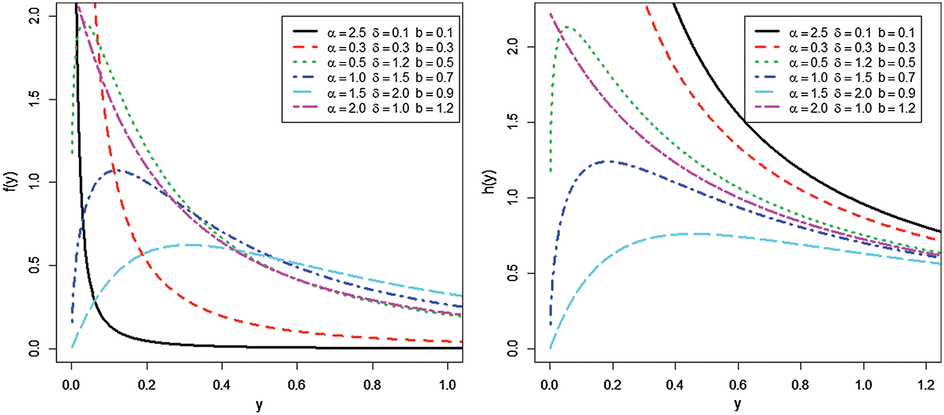
Figure 1: Plots of the pdf and hrf for TLIL model
Fig. 1 gives density and hazard functions plots for specified values of parameters. It is observed that the pdf of the TLIL can be right-skewed, uni-modal and reversed J-shaped. The hazard function can be increasing, decreasing, reversed J-shaped and upside-down bathtub.
2.1 Quantile Function and Median
The quantile function of Y, denoted by Q(u), is defined by inverting Eq. (5) as follows
where u~ U(0,1). Further, the TLIL distribution can be simply simulated from Eq. (8). The median of Y is obtained by putting u = 0.5 in Eq. (8).
Here, we provide the representation of cdf Eq. (5) and pdf Eq. (6) of the TLIL distribution. As mentioned in Hassan et al. [14], the pdf of the TL-G family is expressed as follows:
where
where,
Furthermore, Hassan et al. [14] provided a useful expression of cdf
where
3.1 Probability-Weighted Moments
The probability-weighted moments (PWMs) are less sensitive to outliers. They are utilized to study characteristics of the probability distributions. They are sometimes used when maximum likelihood estimates are unavailable or difficult to compute. The PWMs, denoted by
where, k and h are positive integers. The class of the PWMs of the TLIL is obtained by substituting Eq. (10) and Eq. (12) in Eq. (13) as follows
where;
3.2 Moments and Related Measures
Here, we provide an infinite sum representation for the n-th moment about the origin, inverse moments and incomplete moments of the TLIL model, since it has a pivotal role in the study of the distribution and real data applications. The n-th moment for the TLIL is obtained as follows:
The first four moments are obtained by setting n =1, 2, 3 and 4 in Eq. (15). The n-th central moment (
Based on Eq. (16), we can obtain the skewness and kurtosis measures using the well-known relationships. Further, the moment generating function of the TLIL distribution for |t| < 1, is given by
The m–th inverse moment, for the TLIL distribution is derived by using pdf Eq. (10) as follows:
The harmonic mean of the TLIL distribution can be obtained by using the first inverse moment.
Additionally, the n-th incomplete moment of Y can be obtained from Eq. (10) as follows:
where, B(.,.,t) is the incomplete beta function.
The conditional moments and the mean residual lifetime function are of interest for lifetime models to be obtained. The r-th conditional moment is defined as:
The r-th moment of the residual life of the TLIL distribution is obtained by substituting Eq. (10) in Eq. (20) as follows
where B(.,.,t) is the incomplete beta function. In particular, the mean residual life of the TLIL model is obtained by substituting r =1 in Eq. (21).
Moreover, the reversed residual life (RRL) is defined as the conditional random variable ????−Y|Y≤???? which denotes the time elapsed from the failure of a component given that its life is less than or equal to ????. The r-th moment of the RRL is defined by:
The r-th moment of the RRL of TLIL distribution is obtained by substituting Eq. (10) in Eq. (22) as follows
The mean of RRL (mean waiting time) represents the waiting time elapsed since the failure of an item on condition that this failure had occurred. For, r = 1 in Eq. (23) we obtain the mean of RRL of the TLIL distribution.
The entropy affords a great tool to evaluate the amount of information (or uncertainty) exists in a random observation relating to its parent distribution. A small value of entropy provides the smaller uncertainty in the data. Hassan et al. [14] mentioned that the Rényi entropy of the TL-G distributions is defined as:
where
So, after some manipulation, the Rényi entropy of the TLIL distribution is given by
where, B(.,.) is the beta function.
4 Estimation and Numerical Study
In this section, the ML estimators of the model parameters are derived in the case of complete samples. Also, approximate confidence intervals (CIs) are obtained. Furthermore, a numerical study is conducted.
Suppose that x1, x2,…,xn be the observed values from TLIL distribution whose lifetimes have the pdf Eq. (6). The log-likelihood based on complete sample, is given by
where,
For interval estimation of the parameters, it is known that under regularity conditions, the asymptotic distribution of ML estimators of elements of unknown parameters for
where,
where
In this sub-section, we perform a simulation study to evaluate the behavior of the ML estimates (MLEs). The attitude of the different estimates is checked in terms of their mean square errors (MSEs), standard errors (SEs) and average lengths (ALs) of the CIs. 10000 random samples of sizes 30, 50, 75 and 100 are generated from TLIL distribution. Four sets of parameter values are chosen as;
Table 1: MSEs, SEs and ALs of the MLEs for TLIL distribution
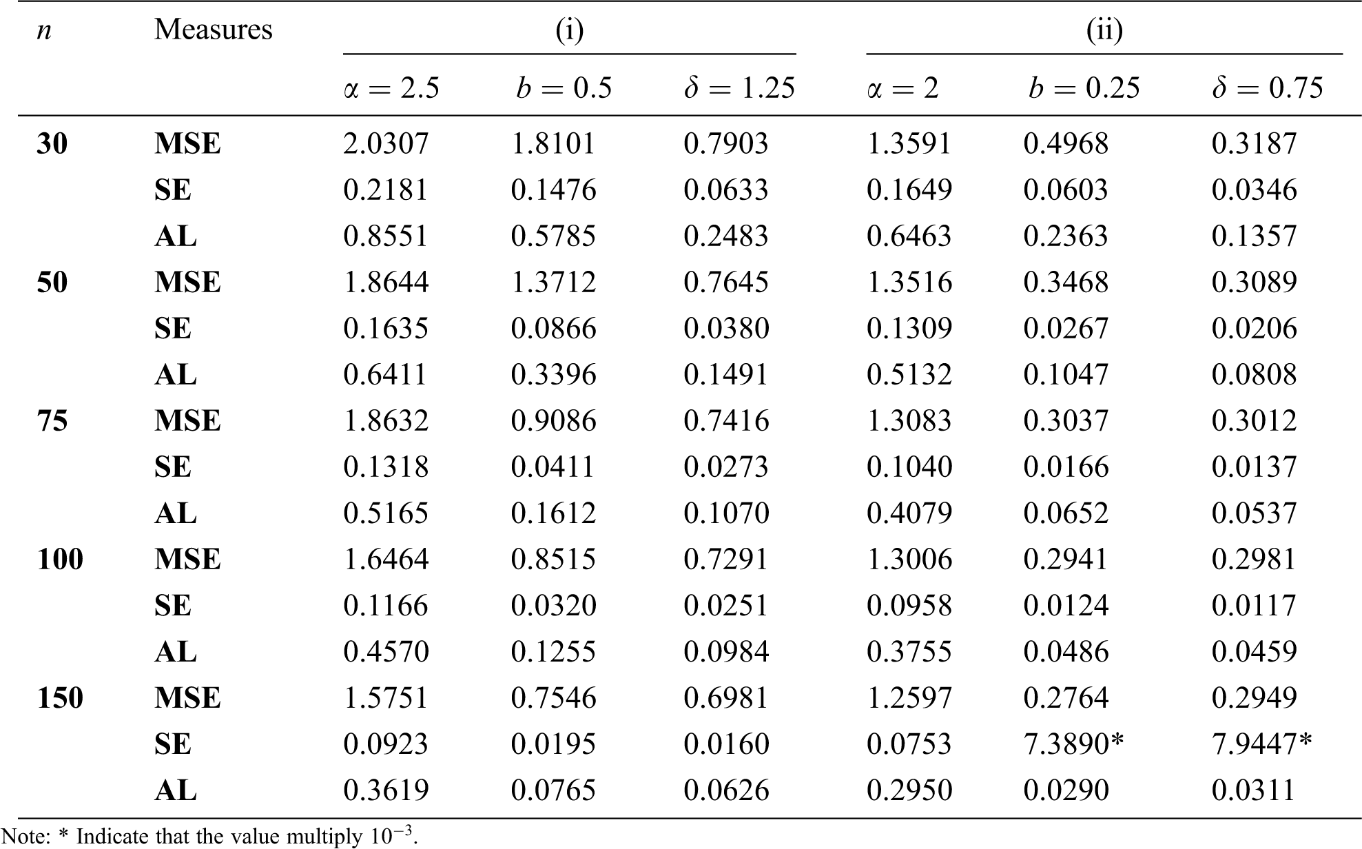
Table 2: MSEs, SEs and ALs of the MLEs for TLIL distribution
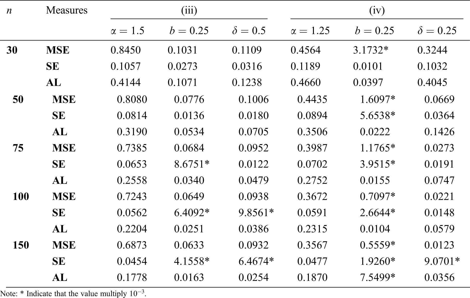
Based on the above tables, we conclude the following
• It is clear that MSEs, SEs and ALs decrease as sample size increases for all estimates.
• The MSEs for
• The MSEs for
• As the value of
• As the value of
• The SEs and ALs for
In this section, we provide the applicability of TLIL distribution by using two real data sets. These data have been used by several authors to show the superiority of other competing models. We also provide a formative evaluation of the goodness of-fit of the models and make comparisons with other distributions. The measures of goodness of fit including; the Akaike information criterion (AIC), Consistent AIC (CAIC), Hannan-Quinn information criterion (HQIC), Anderson-Darling(A∗) and Cramér- von Mises (W∗) are calculated to compare the fitted models. Generally, the best fit to the data that is correspond to the lowest values of these statistics.
The first data set was proposed by Murthy et al. [18], which represents the failure times for a particular windshield device. For these data, we shall compare the TLIL model with the following models: the Zubair Lomax (ZL) [19], gamma-Lomax (GL) [20], exponentiated transmuted generalized Rayleigh (ETGR) [21], transmuted Weibull Lomax (TWL) [22], Kumaraswamy Lomax (KwL) [23], Kumaraswamy Weibull (KwW) [24], McDonald Weibull (McW) [25], beta Weibull (BW) [26] and transmuted Marshall-Olkin Fréchet (TMOFr) [27]. The estimated parameters of these models and the corresponding SEs for windshield data are provided in Tab. 3. The statistics AIC, CAIC, HQIC, A* and W* are mentioned in Tab. 4. The estimated pdf, cdf, sf and PP plots for Aircraft Windshield data of the fitted models are displayed in Fig. 2.
Table 3: MLEs and SEs (in parentheses) for Aircraft Windshield data
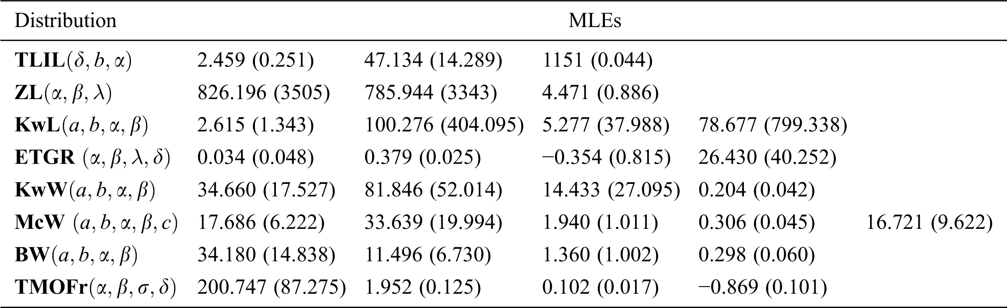
Table 4: The measures of goodness of fit for Aircraft Windshield data
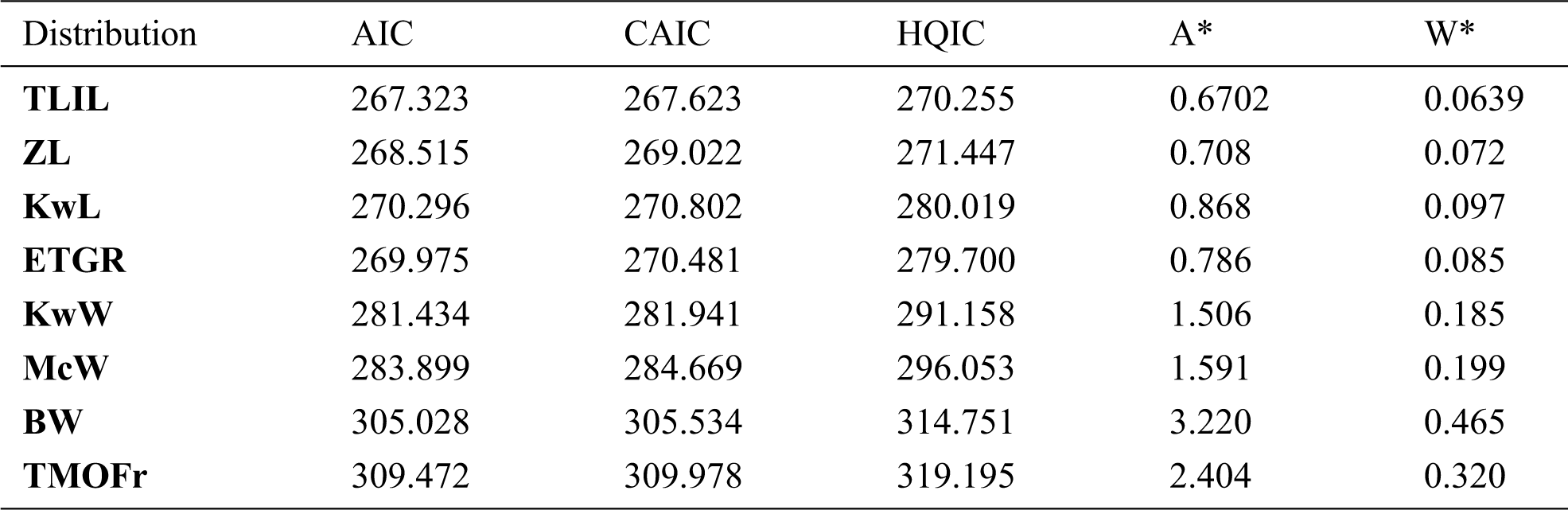
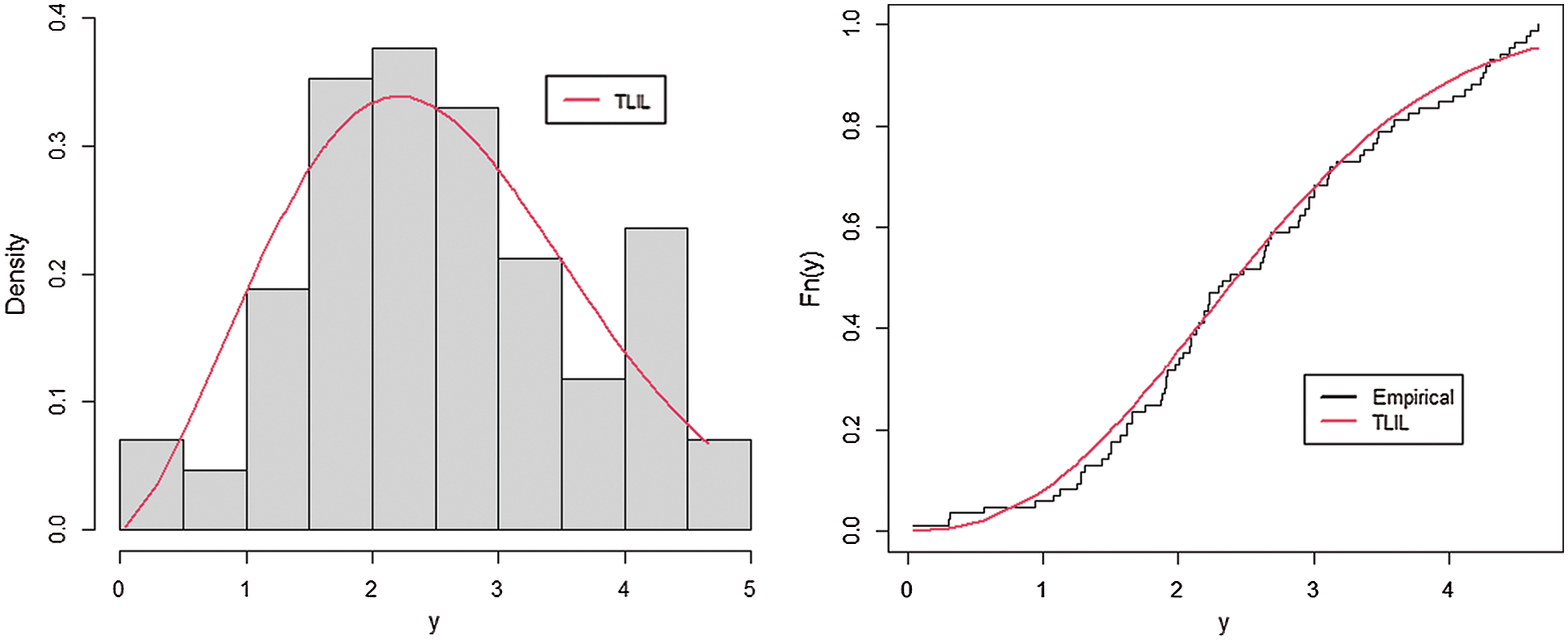
Figure 2: Plots of estimated pdf and cdf for Aircraft Windshield data
It is clear from Tab. 3, Tab. 4 and Fig. 2 that the TLIL provides a better fit to the data and therefore could be chosen as the best model.
This data set describes there mission times (in months) of a random sample of 128 bladder cancer patients studied by Lee et al. [28]. For these data, we compare the fit of the TLIL with some other distributions like; the ZL, transmuted modified Weibull (TMW) distribution [29], transmuted additive Weibull (TAW) distribution [30], generalized inverse gamma distribution distribion [31], beta exponentiated Burr XII (BEBXII) distribution [32], beta Fréchet (BFr) distribution [33] and ETGR distribution The estimated parameters along with their SEs are provided in Tab. 5. The statistics of the fitted models are presented in Tab. 6. We note from Tab. 6 that the TLIL gives the lowest values of AIC, CAIC, HQIC, A∗ and W∗ as compared to the other competitive models. Therefore, TLIL distribution provides the best fit for the cancer patient data. More information can be found in Fig. 3.
Table 5: Estimates and SE (in parentheses) for cancer data
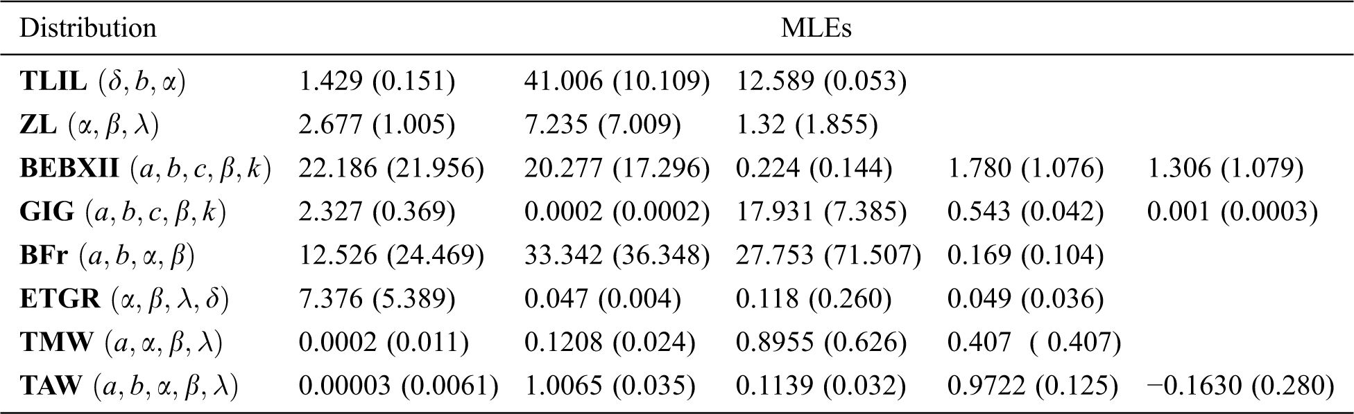
Table 6: The measures of goodness of fit for cancer data
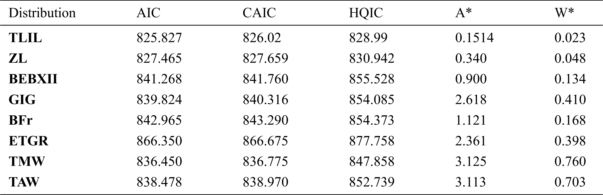
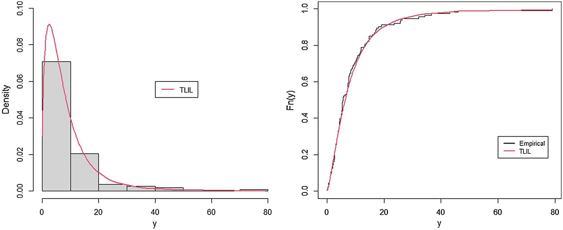
Figure 3: Plots of estimated pdf and cdf plots for cancer data
As seen from Fig. 3 that the TLIL provides a better fit to cancer data and so could be preferred than the other competitive model.
We provide a new three-parameter lifetime distribution depends on the recent truncated Lomax-G family. The new truncated Lomax inverse Lomax model offers flexibility for modeling lifetime data. Expressions of density and distribution functions are obtained as a linear combination of the inverse Lomax distribution. Several mathematical properties of the new model are derived like; probability weighted moments, quantile function, moment generating function, ordinary and incomplete moments, inverse moments, conditional moments, and Rényi entropy. The maximum likelihood method of estimation is employed to obtain the point and approximate confidence interval of population parameters. We assess the accuracy of estimates viz simulation study. Applications to two real data are utilized to illustrate the importance and usefulness of the new model compared to some models.
Acknowledgement: We would like to thank all four reviewers and the academic editor for their interesting comments on the article, greatly improving it in this regard.
Funding Statement: The authors received no specific funding for this study.
Conflicts of Interest: The authors declare that they have no conflicts of interest to report regarding the present review.
1. C. Kleiber and S. Kotz, Statistical size distributions in economics and actuarial sciences. Hoboken, New Jersey: John Wiley and Sons, 2003.
2. S. K. Singh, U. Singh and A. S. Yadav, “Reliability estimation for inverse Lomax distribution under type II censored data using Markov chain Monte Carlo method,” International Journal of Mathematics and Statistics, vol. 17, no. 1, pp. 128–146, 2016.
3. A. S. Yadav, S. K. Singh and U. Singh, “On hybrid censored inverse Lomax distribution: Application to the survival data,” Statistica, vol. 76, no. 2, pp. 185–203, 2016.
4. H. M. Reyad and S. A. Othman, “E- Bayesian estimation of two- component mixture of inverse Lomax distribution based on type- I censoring scheme,” Journal of Advances in Mathematics and Computer Science, vol. 26, no. 2, pp. 1–22, 2018.
5. R. A. R. Bantan, M. Elgarhy, C. Chesneau and F. Jamal, “Estimation of entropy for inverse Lomax distribution under multiple censored data,” Entropy, vol. 22, no. 6, pp. 601, 2020.
6. A. S. Hassan and M. Abd-Allah, “On the inverse power Lomax distribution,” Annals of Data Science, vol. 6, no. 2, pp. 259–278, 2018.
7. A. S. Hassan and R. E. Mohamed, “Weibull inverse Lomax distribution,” Pakistan Journal of Statistics and Operation Research, vol. 15, no. 3, pp. 587–603, 2019.
8. R. A. ZeinEldin, M. A. U. Haq, S. Hashmi and M. Elsehety, “Alpha power transformed inverse Lomax distribution with different methods of estimation and applications,” Complexity, vol. 2020, pp. 1–15, 2020.
9. O. Maxwell, A. U. Chukwu, O. S. Oyamakin and M. A. Khaleel, “The Marshall-Olkin inverse Lomax distribution (MO-ILD) with application on cancer stem cell,” Journal of Advances in Mathematics and Computer Science, vol. 33, no. 4, pp. 1–12, 2019.
10. R. A. ZeinEldin, M. A. ul Haq, S. Hashmi, M. Elsehety and M. Elgarhy, “Statistical inference of odd Fréchet inverse Lomax distribution with applications,” Complexity, vol. 2020, pp. 20, 2020.
11. A. S. Hassan and D. M. Ismail, “Estimation of parameters of Topp-Leone inverse Lomax distribution in presence of right censored samples,” Gazi university Journal of Science. Forthcoming.
12. S. H. Abid and R. K. Abdulrazak, “[0,1] truncated Fréchet-G generator of distributions,” Applied Mathematics, vol. 7, no. 3, pp. 51–66, 2017.
13. R. A. R. Bantan, F. Jamal, C. Chesneau and M. Elgarhy, “Truncated inverted Kumaraswamy generated family of distributions with applications,” Entropy, vol. 21, no. 11, pp. 1089, 2019.
14. A. S. Hassan, M. A. Sabry and A. M. Elsehetry, “A new family of upper-truncated distributions: Properties and estimation,” Thailand Statistician, vol. 18, no. 2, pp. 196–214, 2020.
15. A. S. Hassan, M. A. Sabry and A. M. Elsehetry, “A new probability distribution family arising from truncated power Lomax distribution with application to Weibull model,” Pakistan Journal of Statistics and Operation Research, vol. 16, no. 4, pp. 661–674, 2020.
16. M. A. Aldahlan, J. Farrukh, C. Chesneau, M. Elgarhy and I. Elbatal, “The truncated Cauchy power family of distributions with inference and applications,” Entropy, vol. 22, no. 346, pp. 346, 2020.
17. B. Fisher and A. Kılıcman, “Some results on the gamma function for negative integers,” Applied Mathematics and Information Sciences, vol. 6, no. 2, pp. 173–176, 2012.
18. D. N. P. Murthy, M. Xie and R. Jiang, Weibull models. New York: Wiley, 2004.
19. R. Bantan, A. S. Hassan and M. Elsehetry, “Zubair Lomax distribution: Properties and estimation based on ranked set sampling,” Computers, Materials & Continua, vol. 65, no. 3, pp. 2169–2187, 2020.
20. G. M. Cordeiro, E. M. M. Ortega and B. V. Popović, “The gamma-Lomax distribution,” Journal of Statistical Computation and Simulation, vol. 85, no. 2, pp. 305–319, 2015.
21. A. Z. Afify, Z. M. Nofal and A. N. Ebraheim, “Exponentiated transmuted generalized Rayleigh: A new four parameter Rayleigh distribution,” Pakistan Journal of Statistics and Operation Research, vol. 11, no. 1, pp. 115–134, 2015.
22. A. Z. Afify, Z. M. Nofal, H. M. Yousof, Y. M. El Gebaly and N. S. Butt, “The transmuted Weibull Lomax distribution: Properties and application,” Pakistan Journal of Statistics & Operation Research, vol. 11, no. 1, pp. 135–152, 2015.
23. T. M. Shams, “The Kumaraswamy-generalized Lomax distribution,” Middle-East Journal of Scientific Research, vol. 17, no. 5, pp. 641–646, 2013.
24. G. M. Cordeiro, E. M. M. Ortega and S. Nadarajah, “The Kumaraswamy Weibull distribution with application to failure data,” Journal of the Franklin Institute, vol. 347, no. 8, pp. 1399–1429, 2010.
25. G. M. Cordeiro, E. M. Hashimoto and E. M. Ortega, “McDonald Weibull model,” Statistics Journal of Theoretical and Applied Statistics, vol. 48, no. 2, pp. 256–278, 2014.
26. C. Lee, F. Famoye and O. Olumolade, “Beta-Weibull distribution: Some properties and applications to censored data,” Journal of Modern Applied Statistical Methods, vol. 6, no. 1, pp. 173–186, 2007.
27. A. Z. Afify, G. G. Hamedani, I. Ghosh and E. M. Mead, “The transmuted Marshall-Olkin Fréchet distribution: Properties and applications,” International Journal of Probability and Statistics, vol. 4, no. 4, pp. 132–148, 2015.
28. E. T. Lee and J. W. Wang, Statistical Methods for Survival Data Analysis, 3rd edition. New York: Wiley, 2003.
29. M. S. Khan and R. King, “Transmuted modified Weibull distribution: A generalization of the modified Weibull probability distribution,” European Journal of Pure and Applied Mathematics, vol. 6, no. 1, pp. 66–88, 2013.
30. I. Elbatal and G. Aryal, “On the transmuted additive Weibull distribution,” Austrian Journal of Statistics, vol. 42, no. 2, pp. 117–132, 2013.
31. M. Mead, “Generalized inverse Gamma distribution and its application in reliability,” Communications in Statistics-Theory and Methods, vol. 44, no. 7, pp. 1426–1435, 2015.
32. M. Mead, “A new generalization of Burr XII distribution,” Journal of Statistics: Advances in Theory and Applications, vol. 12, no. 2, pp. 53–73, 2014.
33. S. Nadarajah and A. K. Gupta, “The beta Fréchet distribution,” Far East Journal of Theoretical Statistics, vol. 14, no. 1, pp. 15–24, 2004.
 | This work is licensed under a Creative Commons Attribution 4.0 International License, which permits unrestricted use, distribution, and reproduction in any medium, provided the original work is properly cited. |