Intelligent Automation & Soft Computing DOI:10.32604/iasc.2021.017652
Article

A New Four-Parameter Moment Exponential Model with Applications to Lifetime Data

Abdullah Ali H. Ahmadini1, Amal S. Hassan2, Rokaya E. Mohamed3,*, Shokrya S. Alshqaq4 and Heba F. Nagy5

1Department of Mathematics, Faculty of Science, Jazan University, Jazan, Saudi Arabia
2Faculty of Graduate Studies for Statistical Research, Department of Mathematical Statistics, Cairo University, Egypt
3Sadat Academy for Management Sciences, Department of Mathematics, Statistics and Insurance, Cairo, Egypt
4Department of Mathematics, Faculty of Science, Jazan University, Jazan, Saudi Arabia
5Faculty of Graduate Studies for Statistical Research, Department of Mathematical Statistics, Cairo University, Egypt
*Corresponding Author: Rokaya E. Mohamed. Email: rokayaelmorsy@gmail.com
Received: 01 February 2021; Accepted: 06 March 2021

Abstract: In this research article, we propose and study a new model the so-called Marshal-Olkin Kumaraswamy moment exponential distribution. The new distribution contains the moment exponential distribution, exponentiated moment exponential distribution, Marshal Olkin moment exponential distribution and generalized exponentiated moment exponential distribution as special sub-models. Some significant properties are acquired such as expansion for the density function and explicit expressions for the moments, generating function, Bonferroni and Lorenz curves. The probabilistic definition of entropy as a measure of uncertainty called Shannon entropy is computed. Some of the numerical values of entropy for different parameters are given. The method of maximum likelihood is adopted for estimating the model parameters. We study the behavior of the maximum likelihood estimates for the model parameters using simulation study. A numerical study is performed to evaluate the behavior of the estimates with respect to their absolute biases, standard errors and mean square errors for different sample sizes and for different parameter values. Further, we conclude that the maximum likelihood estimates of the Marshal-Olkin Kumaraswamy moment exponential distribution perform well as the sample size increases. We take advantage of applied studies and offer two applications to real data sets that prove empirically the power of adjustment of the new model when compared to other lifetime distributions.

Keywords: Marshal-Olkin Kumaraswamy family; moment exponential distribution; quantile function; maximum likelihood estimation

1  Introduction

The modeling and analysis of lifetimes are important aspects of statistical work in a wide variety of technological fields. The procedure of adding one or two shape parameters to a class of distributions to obtain more flexibility, especially for studying tail behavior, is a well-known technique in the statistical literatures. Marshall et al. [1] proposed a method of adding a shape parameter to a family of distributions and many authors used their method to extend several well-known distributions.

The cumulative distribution function (cdf) and the probability density function (pdf) of the Marshall- Olkin (MO) family are defined as follows:

FMO(x;α,ζ)=G(x;ζ)/G(x;ζ)[1−α¯(G¯(x;ζ))][1−α¯(G¯(x;ζ))], (1)

and,

fMO(x;α,ζ)=αg(x;ζ)/αg(x;ζ)[1−α¯(G¯(x;ζ))]2[1−α¯(G¯(x;ζ))]2, (2)

where, α>0, α¯=1−α, and G¯(x;ζ)=1−G(x;ζ) is the survival function. The parameter α¯ is known as a tilt parameter and interpreted α¯ in terms of the behavior of the hazard rate function (hrf) of F¯(x). This ratio is increasing in x for α¯≥1 and decreasing in x for α¯∈(0,1) (see [2]). It is obvious that many new families can be derived from MO set up by considering different baseline distributions-G in Eq. (1). These new families are usually termed as MO extended-G distribution. The generalized MO proposed in [3] through exponentiating the MO survival function is defined as follows:

F¯GMO(x;α,b,ζ)=[α(G¯(x;ζ))1−α¯(G¯(x;ζ))]b. (3)

Tahir et al. [4] presented another generalization by exponentiating the cdf of the MO family; as follows:

FG2MO(x;α,b,ζ)=[1−α(G¯(x;ζ))1−α¯(G¯(x;ζ))]b. (4)

[For more on MO distributions see [5–13]]. Cordeiro et al. [14] defined the Kumaraswamy-G (Kw-G) class with the cdf and pdf given by

FKw(x;a,b,ζ)=1−[1−(G(x;ζ))a]b, (5)

and,

fKw(x;a,b,ζ)=abg(x;ζ)(G(x;ζ))a−1[1−(G(x;ζ))a]b−1, (6)

where a > 0 and b > 0 are shape parameters, in addition to those in the baseline distribution which partly govern skewness and variation in tail weights. Handique et al. [15] proposed a new extension of the MO family by considering the cdf and pdf of Kw-G distribution in (5) and (6) and call it MO Kumaraswamy-G (MOKw-G) distribution with cdf and pdf given by:

FMOKw(x;a,b,α,ζ)=1−[1−(G(x;ζ))a]b1−α¯[1−(G(x;ζ))a]b, (7)

and,

fMOKw(x;a,b,α,ζ)=abαg(x;ζ)(G(x;ζ))a[1−(G(x;ζ))a]b−1(1−α¯[1−(G(x;ζ))a]b)2, (8)

where G(x;ζ) is the baseline cdf depending on a parameter vector ζ; and a,b>0, are additional shape parameters. The MOKw-G family generalizes the Kw-G family as well as the MO family.

The exponential distribution is a very popular statistical model and, probably, is one of the parametric models that most extensively applied in several fields [16]. Due to its importance, several studies introducing and/or studying extensions of the exponential distribution are available in the literatures. Some forms of exponential distribution are; the exponentiated exponential [17,18], beta exponential [19], beta generalized exponential [20], moment exponential [21], exponentiated moment exponential [22], generalized exponentiated moment exponential [23], extended exponentiated exponential [24], MO exponential Weibull [25], MO generalized exponential (MOGE) [26], MO length-biased exponential (MOLBE) [27], alpha power transformed extended exponential [28] and MO Kumaraswamy exponential (MOKwE) [29] distributions.

Moment distributions have a vital role in mathematics and statistics, in particular in probability theory, in the perspective research related to ecology, reliability, biomedical field, econometrics, survey sampling and in life-testing. Dara et al. [21] proposed the moment exponential (ME) distribution through assigning weight to the exponential distribution. They showed that their proposed model is more flexible model than the exponential distribution. The pdf of the ME distribution is specified by:

g(x;β)=xβ2e−xβ,β,x>0, (9)

where, β is the scale parameter. The cdf corresponding to (9) is

G(x;β)=1−(1+xβ)e−xβ,β,x>0. (10)

In this paper, we introduce and study the MO Kumaraswamy ME (MOKwME) distribution. The MOKwME model includes as special cases the generalized exponentiated ME (GEME), exponentiated ME (EME), MOLBE, Kumaraswamy ME (KwME) and ME distributions, which are very important statistical models, especially for applied works. It is interesting to observe that its hazard rate function can be, increasing, decreasing, and upside-down bathtub. Accordingly, it can be used effectively to analyze lifetime data sets. Some statistical properties of the proposed model are provided. Maximum likelihood (ML) estimators of the model parameters are presented. A simulation study and an application of the suggested model on real life data set are given.

2  Model Formulation

The cdf and pdf of the MOKwME distribution are obtained by substituting (9) and (10) in (7) and (8) as follows:

F(x;ψ)=1−[1−(1−Λ(x,β))a]b1−α¯[1−(1−Λ(x,β))a]b,a,b,α,β>0,x>0, (11)

and,

f(x;ψ)=abαxβ2e−xβ(1−Λ(x,β))a−1(1−(1−Λ(x,β))a)b−1(1−α¯[1−(1−Λ(x,β))a]b)−2. (12)

where, Λ(x,β)=(1+x/xββ)e−xβ, ψ=(a,b,α,β) is a set of parameters. A random variable X has MOKwME distribution will be denoted by X~ MOKwME (a,b,α,β). The MOKwME distribution is a very flexible model that approaches to some distributions as follows:

•   For α=0 and b=1, we obtain EME distribution presented in [22]

•   For a=1 and b=1, we obtain MOLBE distribution presented in [27].

•   For α=0,b=1, and y=x1/δ we obtain, GEME distribution presented in [23].

•   For a=1, b=1, and α=0, we obtain, ME distribution presented in [21].

•   For α=1, we obtain, KwME distribution as a new model.

Next, we provide a simple motivation for the MOKwME distribution in the medical context as follows (see [15]): Consider a random sample X1, X2,…, XN, where the Xi’s, i =1,2,…,N, be a sequence of identically independent distributed random variables with survival function [1−(1−Λ(x,β))a]b then

•   If N has a geometric distribution with parameter α;(0<α<1) independent of Xi’s then the density of the random variable W1= min( X1, X2,…,XN ) is that MOKwME (a,b,α,β).

•   If N has a geometric distribution with parameter 1/α;(α>1) independent of, Xi’s then density of the random variable W2 = max( X1, X2,…, XN ) distributed as MOKwME (α−1,a,b,β).

This setup is usually common in oncology, where N represents the amount of cells with metastasis potential and Xi denotes the time for the ith cell to metastasis. So, X represents the recurrence time of the cancer.

The survival and hazard rate functions of X are given, respectively, as follows:

F¯(x;ψ)=α[1−(1−Λ(x,β))a]b{1−α¯[1−(1−Λ(x,β))a]b}−1, (13)

and

h(x;ψ)=abβ2xe−xβ(1−Λ(x,β))a−1(1−(1−Λ(x,β))a)−1{1−α¯[1−(1−Λ(x,β))a]b}−1. (14)

Plots of the pdf and hrf of the MOKwME distribution are displayed in Figs. 1 and 2, respectively, for different values of parameters. As seen from Fig. 1, the shapes of the pdf take different forms. Also, it is clear from Fig. 2 that the shapes of the hrf are reversed J-shaped, decreasing, increasing and upside-down bathtub at some selected values of parameters.

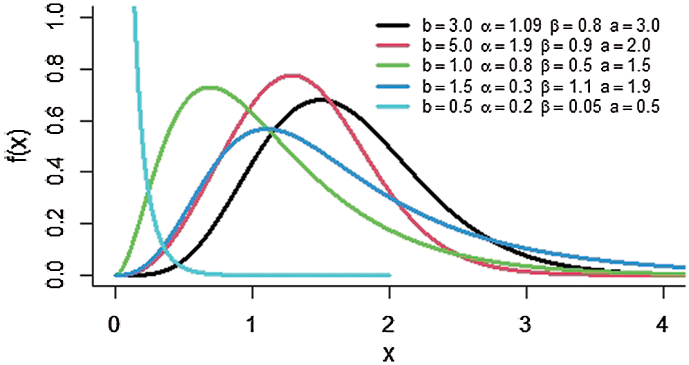
Figure 1: The pdf of the MOKwME distribution for some values of parameters

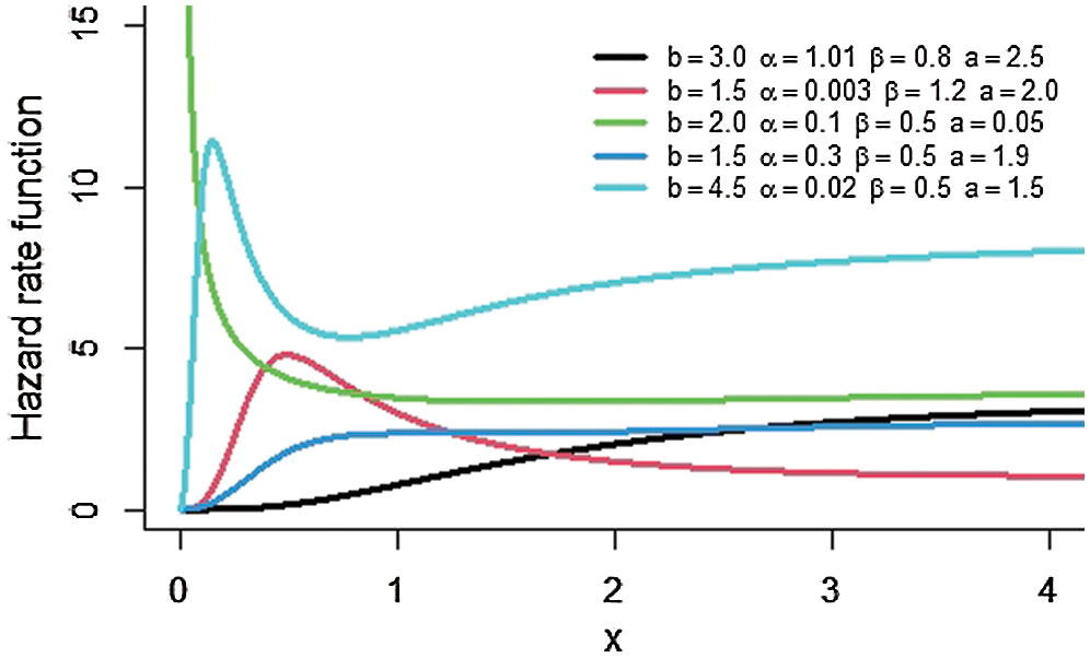
Figure 2: The hrf of the MOKwME distribution for some values of parameters

3  Statistical Properties

3.1 Expansion

Here, explicit expression for the MOKwME density function is provided. Since, the binomial expansion, for real non-integer value of k, is given by:

(1−y)−k=∑j=0∞Γ(k+j)yjΓ(k)j!,|y|<1,k>0. (15)

Using (15) in pdf (12), we obtain

f(x;ψ)=∑j=0∞(j+1)abα(α¯)jxβ2e−xβ(1−(1+xβ)e−xβ)a−1(1−(1−(1+xβ)e−xβ)a)b(j+1)−1. (16)

Again applying the binomial expansion in "previous equation", we obtain

f(x;ψ)=∑i,j=0∞(−1)i(j+1)abα(α¯)j(b(j+1)−1i)xβ2e−xβ(1−(1+xβ)e−xβ)a(i+1)−1. (17)

Hence the pdf of MOKwME distribution can be written as follows:

f(x;ψ)=∑i,j=0∞wi,ja(i+1)g(x;β)(G(x;β))a(i+1)−1, (18)

where, wi,j=bα(α¯)j(i+1)(−1)i(j+1)(b(j+1)−1i).

Eq. (18) reveals that the MOKwME density function is a linear mixture of EME density functions with power parameter a(i+1) .

3.2 Moments

Here, we discuss the sth moment for the MOKwME distribution. The sth moment for the MOKwME distribution about zero is derived by using pdf (18) as follows:

μs′=∑i,j=0∞wi,ja(i+1)β2∫0∞xs+1e−xβ(1−(1+xβ)e−xβ)a(i+1)−1dx. (19)

Suppose v=x/xβ,β, then μs′ can be written as follows:

μs′=∑i,j=0∞wi,ja(i+1)βs∫0∞vs+1e−v(1−(1+v)e−v)a(i+1)−1dv. (20)

Using binomial expansion, then

μs′=∑i,j,ℓ=0∞∑m=0ℓbi,j,m,ℓβsΓ(s+m+2)(ℓ+1)s+m+2,s=1,2,..., (21)

where bi,j,m,ℓ=a(i+1)(−1)ℓ(a(i+1)−1ℓ)(ℓm).

The mean of the MOKwME distribution is obtained by putting s =1 in (21). The sth central moment (μs ) of X is given by

μs=E(X−μ1′)s=∑i=0s(−1)i(si)(μ1′)iμs−i′. (22)

3.3 Incomplete Moments

The sth incomplete moment, say τs(t) is defined by:

τs(t)=∫−∞t⁡xsf(x)dx. (23)

Hence, the sth moment of MOKwME is derived by substituting (18) in (23) as follows:

τs(t)=∑i,j,ℓ=0∞∑m=0ℓbi,j,ℓ,mβsγ(s+m+2(ℓ+1)s+m+2,tβ), (24)

where γ(k,t)=∫0txk−1e−kdx is the lower incomplete gamma function. The Bonferroni and Lorenz curves and the Gini indices have applications in economics, reliability, demography, insurance and medicine (see [30]). The Lorenz curve of MOKwME distribution is given as follows:

L[X]=1μ′1∫0xtf(t)dt=∑i,j,ℓ=0∞∑m=0ℓbi,j,ℓ,mγ(m+3(ℓ+1)m+3,xβ)∑i,j,ℓ=0∞∑m=0ℓbi,j,ℓ,mΓ(m+3)(ℓ+1)m+3. (25)

The Bonferroni curve of MOKwME distribution is obtained as

BF[X]=1μ′1F(x)∫0xtf(t)dt=1F(x;ψ)∑i,j,ℓ=0∞∑m=0ℓbi,j,ℓ,mγ(m+3(ℓ+1)m+3,xβ)∑i,j,ℓ=0∞∑m=0ℓbi,j,ℓ,mΓ(m+3)(ℓ+1)m+3. (26)

3.4 Moments of Residual Life Function

The residual life plays an important role in life testing situations and reliability theory. The nth moment of the residual life is defined by:

ϖn(t)=E[(X−t)n|X>t]=1F¯(t)∫t∞(x−t)nf(x)dx. (27)

Using the binomial expansion and pdf (18), then ϖn(t) can be written as follows:

ϖn(t)=1F¯(t;ψ)∑r=0n∑i,j=0∞(nr)wi,ja(i+1)(−t)n−r∫t∞xr+1β2e−xβ(1−(1+xβ)e−xβ)a(i+1)−1dx. (28)

So, after simplification the nth moment of the residual life of MOKwME distribution is obtained as follows:

ϖn(t)=1F¯(t;ψ)∑r=0n∑i,j,ℓ=0∞∑m=0ℓ(nr)bi,j,ℓ,m(−t)n−rβrΓ(r+m+2(ℓ+1)r+m+2,tβ), (29)

where Γ(k,t)=∫t∞xk−1e−kdx is the upper incomplete gamma and F¯(t;ψ) is the survival function of MOKwME distribution In particular, the mean residual life (MRL) which represents the expected additional life length for a unit which is alive at age t is obtained by substituting n =1 in (29).

3.5 Quantile

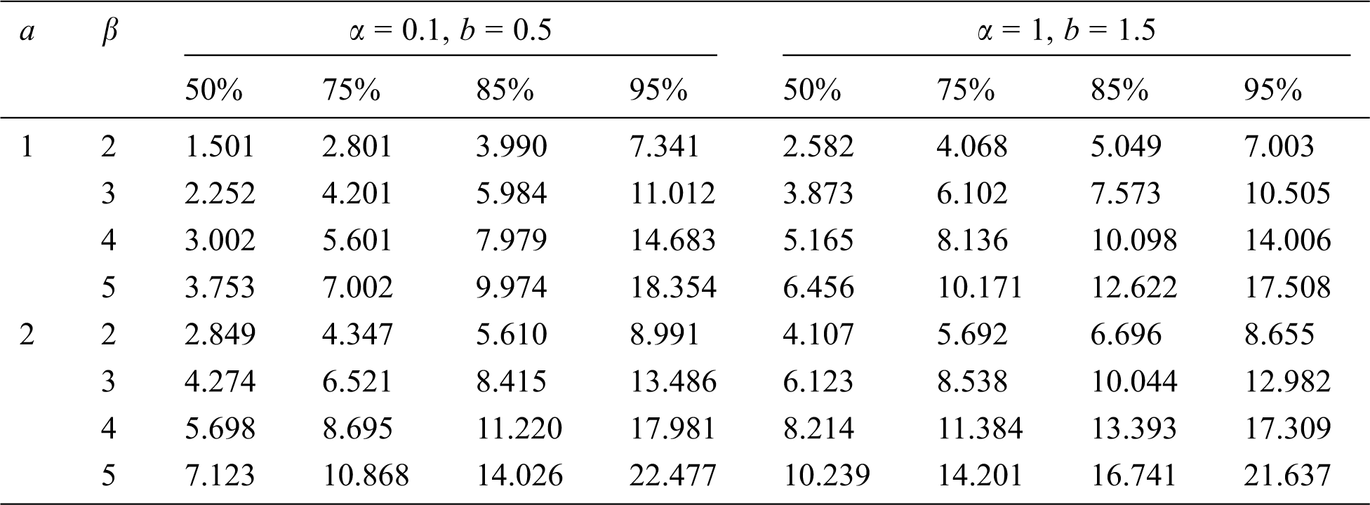
The P-th quantile function (also called the percentile of order p) of the MOKwME distribution is of the form:

1−[1−(1−Λ(x,β))a]b1−α¯[1−(1−Λ(x,β))a]b=P. (30)

In particular, the median, denoted by M, can be obtained from (30) by substituting P = 0.5 and solving the following:

1−[1−(1−Λ(x,β))a]b1−α¯[1−(1−Λ(x,β))a]b=0.5. (31)

Solving the Eq. (30) numerically, the percentage points are computed for some selected values of the parameters. These values are provided in Tab. 1.

Table 1: Percentage points for a,b,α and β

4  Shannon Entropy

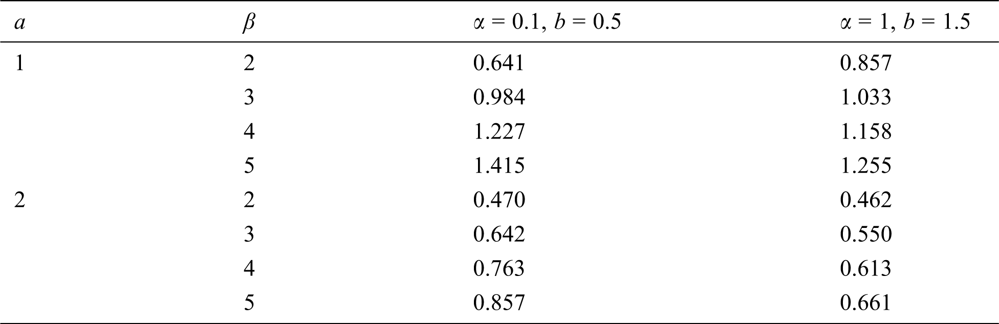
Shannon [31] introduced the probabilistic definition of entropy as a measure of uncertainty. It is also a useful instrument for comparing two or more distributions. The Shannon entropy of a random variable X is defined by:

SH(f)=−(∫−∞∞f(x)log⁡(f(x))dx). (32)

The Shannon entropy for the MOKwME distribution with pdf (12) is as follows:

SH(f)=−∫0∞abαxβ2e−xβ(1−Λ(x,β))a−1(1−(1−Λ(x,β))a)b−1(1−α¯[1−(1−Λ(x,β))a]b)−2log[abαxβ2e−xβ(1−Λ(x,β))a−1(1−(1−Λ(x,β))a)b−1(1−α¯[1−(1−Λ(x,β))a]b)−2]dx. (33)

Since the theoretical result of entropy is not in a closed form, some of the numerical values of entropy for different parameters are given in Tab. 2.

Table 2: Shannon Entropy for some values of a,b,α and β

5  Maximum Likelihood Estimators

We consider the estimation of the unknown parameters of the MOKwME distribution using the ML method. Let X1, X2, …, Xn be the observed values from the MOKwME distribution with set of parameters ψ=(a,b,α,β)T. The log-likelihood function, denoted by LnL, based on complete sample for the vector of parameters ψ can be expressed as

LnL=nln⁡a+nln⁡b+nln⁡α−2nln⁡β+∑i=1nlnxi−∑i=1nxiβ+(a−1)∑i=1nln(1−Λ(xi,β))+(b−1)∑i=1nln⁡(1−(1−Λ(xi,β))a)−2∑i=1nln(1−α¯[1−(1−Λ(xi,β))a]b), (34)

The partial derivatives of the log-likelihood function with respect to a,b,α and β components of the score vector U(ψ)=∂LnL/∂LnL∂ψ∂ψ=(U(a),U(b),U(α),U(β))T can be obtained as follows:

U(a)=na+∑i=1nln⁡(1−Λ(xi,β))−(b−1)∑i=1nln⁡(1−Λ(xi,β))((1−Λ(xi,β))−a−1)−2∑i=1nα¯bln⁡(1−Λ(xi,β))(1−Λ(xi,β))a[1−(1−Λ(xi,β))a]b−1(1−α¯[1−(1−Λ(xi,β))a]b), (35)

U(b)=nb+∑i=1nln⁡(1−(1−Λ(xi,β))a)+2∑i=1nln⁡[1−(1−Λ(xi,β))a]((1/1α¯α¯)[1−(1−Λ(xi,β))a]−b−1), (36)

U(α)=nα+2∑i=1n[1−(1−Λ(xi,β))a]b(1−α¯[1−(1−Λ(xi,β))a]b), (37)

U(β)=−2nβ+∑i=1nxiβ2−∑i=1n(a−1)(1−Λ(xi,β)∂Λ(xi,β)∂β+∑i=1na(b−1)(1−Λ(xi,β))a−1(1−(1−Λ(xi,β))a)∂Λ(xi,β)∂β+2∑i=1nabα¯[1−(1−Λ(xi,β))a]b−1(1−Λ(xi,β))a−1(1−α¯[1−(1−Λ(xi,β))a]b)∂Λ(xi,β)∂β, (38)

and,

∂Λ(xi,β)∂β=xi2β3e−xiβ. (39)

The ML estimators of the model parameters are determined by solving the non-linear equations U(a)=0,U(b)=0,U(α)=0, and U(β)=0. These equations cannot be solved analytically and statistical software can be used to solve them numerically via iterative technique.

6  Simulation Study

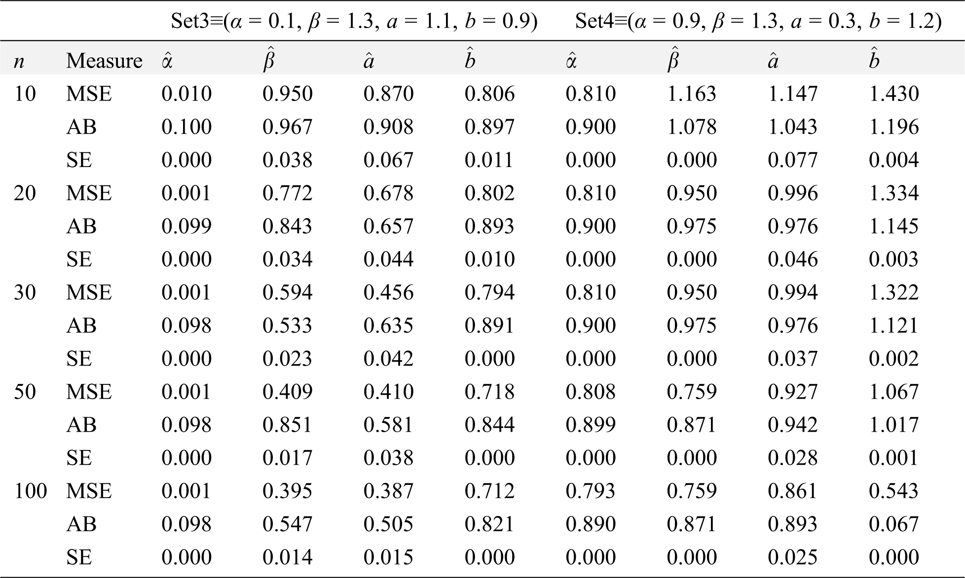
A numerical study is performed to evaluate the performance of the estimates with respect to their absolute biases (ABs), standard errors (SEs) and mean square errors (MSEs) for different sample sizes and for different parameter values. The numerical procedures are described through the following steps:

Step 1: A random sample X1,…,Xn of sizes n =10, 20, 30, 50 and 100 are selected, these random samples are generated from the MOKwME distribution.

Step 2: Four different set values of the parameters are selected as, Set1≡(α=0.3,β=0.8,a=0.8,b=0.5), Set2≡ (α=0.6,β=0.8,a=0.5,b=0.7), Set3≡ (α=0.1,β=1.3, a=1.1, b=0.9) and Set4≡(α=0.9,β=1.3,a=0.3,b=1.2).

Step 3: For each sample size, the ML estimates (MLEs) of α, β, a and b are computed.

Step 4: Steps from 1 to 3 are repeated 1000 times, then, the ABs, SEs and MSEs of the estimates are computed.

Numerical results are reported in Tabs. 3 and 4, from these tables, the following observations can be detected on the behavior of estimated parameters from the MOKwME distribution.

•   The ABs, SEs and MSEs decrease as sample sizes increase (see Tabs. 3 and 4).

•   The ABs of a decrease as the value of b increases (see Tab. 3). Also, the ABs of β increase as the value of β increases, in approximately, most of the situations.

•   For fixed values of β and as the values of b and α increase, the ABs and MSEs are decreasing, in approximately most of situations (see Tab. 3). As the values of α increase and for fixed values of β, the ABs and MSEs for all estimates decrease (see Tab. 4).

Table 3: ABs, SEs and MSEs of MOKwME parameter estimates for Set 1and Set 2

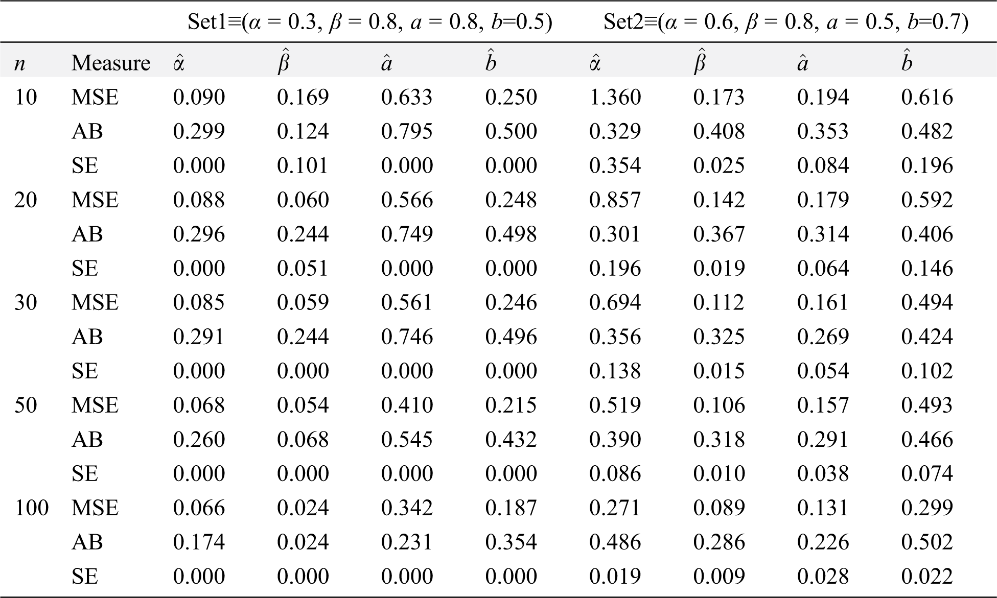
Table 4: ABs, SEs and MSEs of MOKwME parameter estimates for Set 3and Set 4

7  Real Data Applications

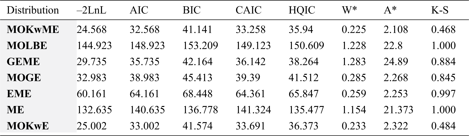
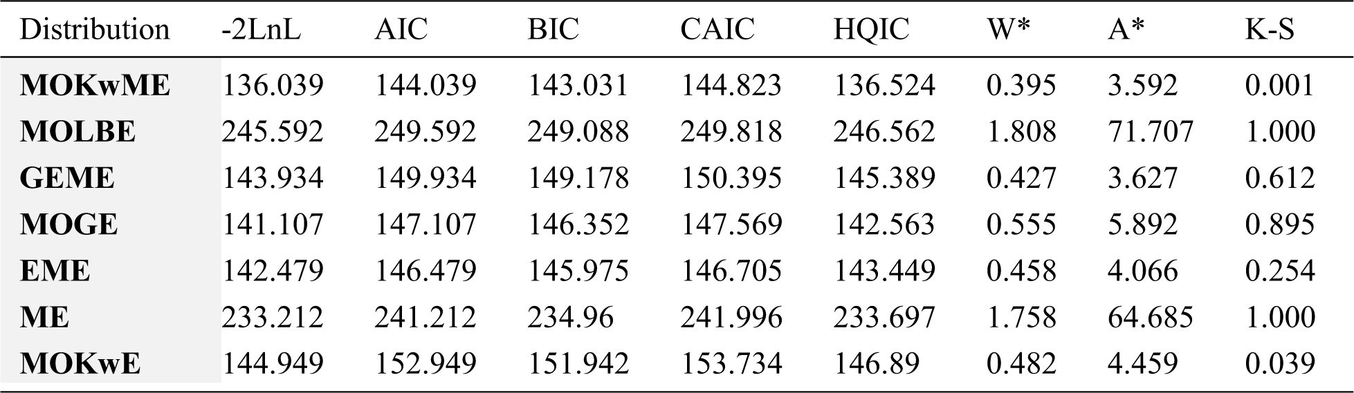
In this section, we fit the MOKwME distribution into two distinct real data sets and we compare the performance with those of MOLBE, GEME, MOGE, EME, ME and MOKwE distributions. In each real data set, the MLEs and their corresponding SEs (in parentheses) of the model parameters are obtained. -2 log-likelihood (-2LnL), Akaike information criterion (AIC), the correct Akaike information criterion (CAIC), Bayesian information criterion (BIC), Hannan-Quinn information criterion (HQIC), Anderson-Darling (A*) statistic, Cramér- von Mises (W*) statistic and Kolmogorov-Smirnov (K-S) statistic are used to assess the effectiveness of the models. The model with the smallest value of these measures gives a better representation of the data set than the others.

First Real Data Set: The first data refer to Smith et al. [32] which represent the strengths of 1.5 cm glass fibers, measured at the National Physical Laboratory, England. The data are:

0.55, 0.93, 1.25, 1.36, 1.49, 1.52, 1.58, 1.61, 1.64, 1.68, 1.73, 1.81, 2.0, 0.74, 1.04, 1.27, 1.39, 1.49, 1.53, 1.59, 1.61, 1.66, 1.68, 1.76, 1.82, 2.01, 0.77, 1.11, 1.28, 1.42, 1.50, 1.54, 1.60, 1.62, 1.66, 1.69, 1.76, 1.84, 2.24, 0.81, 1.13, 1.29, 1.48, 1.5, 1.55, 1.61, 1.62, 1.66, 1.70, 1.77, 1.84, 0.84, 1.24, 1.30, 1.48, 1.51, 1.55, 1.61, 1.63, 1.67, 1.70, 1.78, 1.89.

The MLEs and their corresponding SEs (in parentheses) of the model parameters are listed in Tab. 5. Also, the above suggested statistical measures of all models are listed in Tab. 6. It is observed, from Tab. 6, that the MOKwME distribution gives a better fit than other fitted models.

Table 5: MLEs of all models and the corresponding SEs (in parentheses) for the first data

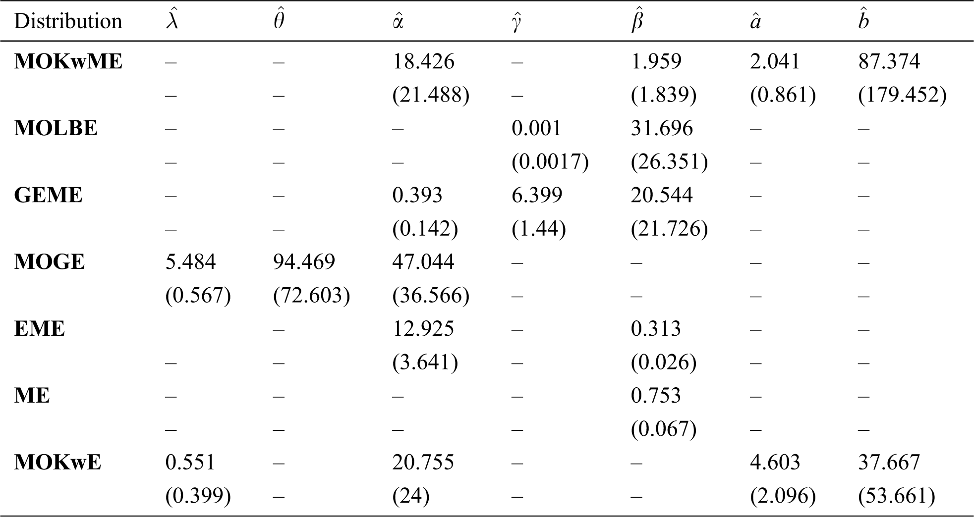
Table 6: Statistics measures for the first data

The empirical pdf and estimated cdf for the first data set are provided in Figs. 3 and 4.

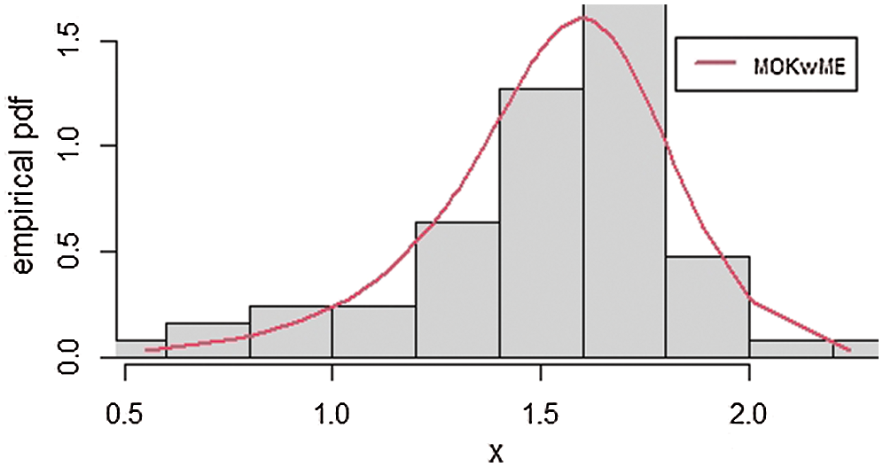
Figure 3: The empirical pdf of the MOKwME distribution for the first real data

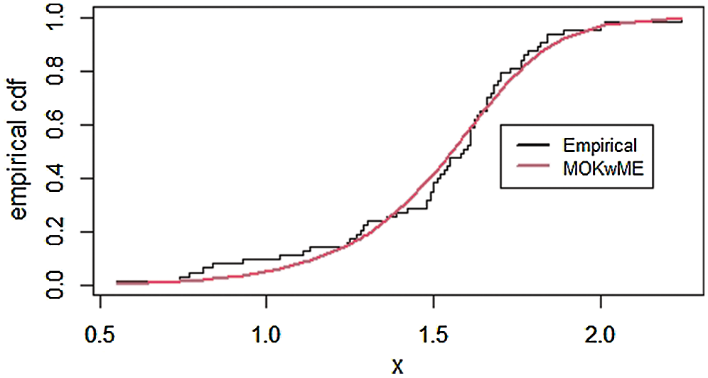
Figure 4: The empirical cdf of the MOKwME distribution for the first real data

Second Real Data: The second data were discussed in Ristić et al. [26], which represent the strength data measured in GPA, the single carbon fibers, and impregnated 1000-carbon fiber tows. Single fibers were tested under tension at gauge length 1 mm. The data are:

2.247, 2.64, 2.908, 3.099, 3.126, 3.245, 3.328, 3.355, 3.383, 3.572, 3.581, 3.681, 3.726, 3.727, 3.728, 3.783, 3.785, 3.786, 3.896, 3.912, 3.964, 4.05, 4.063, 4.082, 4.111, 4.118, 4.141, 4.246, 4.251, 4.262, 4.326, 4.402, 4.457, 4.466, 4.519, 4.542, 4.555, 4.614, 4.632, 4.634, 4.636, 4.678, 4.698, 4.738, 4.832, 4.924, 5.043, 5.099, 5.134, 5.359, 5.473, 5.571, 5.684, 5.721, 5.998, 6.06.

The MLEs and the SEs of the model parameters are listed in Tab. 7 whereas Tab. 8 gives the statistics measures of all models. It is observed, from Tab. 8, that the MOKwME distribution gives a better fit than other fitted models.

Table 7: MLEs of all models and the corresponding SEs (in parentheses) for the second data

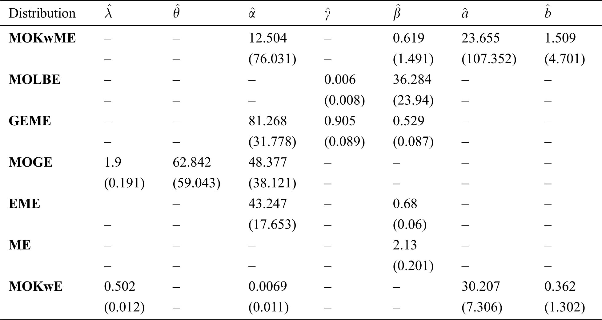
Table 8: Statistics measures for the second data

The empirical pdf and cdf for the second data set are provided in Figs. 5 and 6.

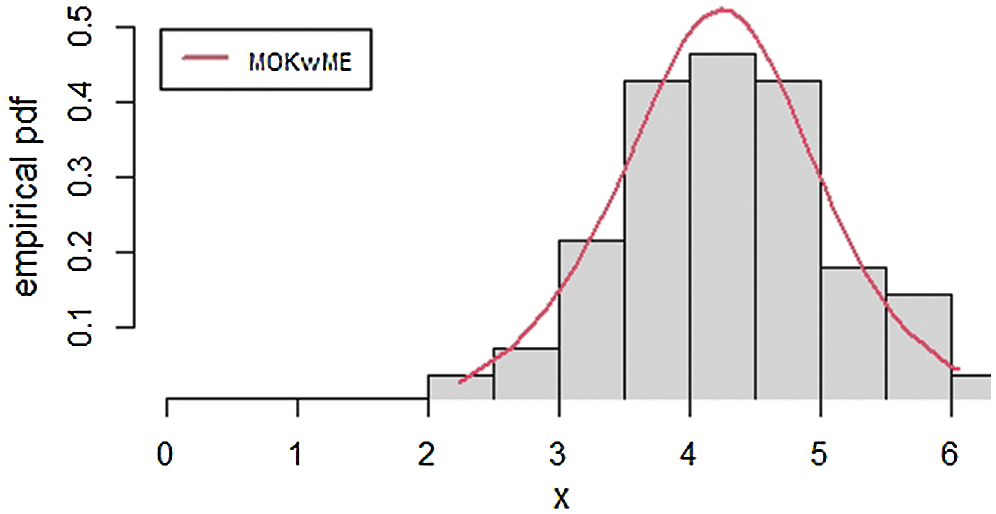
Figure 5: The empirical pdf of the MOKwME distribution for the second real data

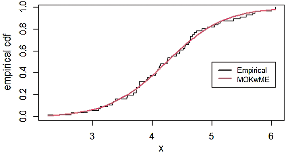
Figure 6: The empirical cdf of the MOKwME distribution for the second real data

8  Concluding Remarks

In this paper, we introduce a new probability model called the Marshal-Olkin Kumaraswamy moment exponential. The new model includes; exponentiated moment exponential, generalized exponentiated moment exponential, Marshall-Olkin length-biased exponential and moment exponential distributions. At the same time, it contains the Kumaraswamy moment exponential distribution as a new model. We study some of its structural properties including an expansion for the density function and explicit expressions for the moments, generating function, Bonferroni and Lorenz curves. The maximum likelihood method is employed for estimating the model parameters. The usefulness of the new model is illustrated by means of an application to real data set.

Acknowledgement: The authors would like to thank the editor and the anonymous referees for their valuable and very constructive comments, which have greatly improved the contents of the paper

Funding Statement: The authors received no specific funding for this study.

Conflicts of Interest: The authors declare no conflict of interest.

References

 1.  A. W. Marshall and I. Olkin, “A new method for adding a parameter to a family of distributions with application to the exponential and Weibull families,” Biometrika, vol. 84, no. 3, pp. 641–652, 1997. [Google Scholar]

 2.  A. K. Nanda and S. Das, “Stochastic orders of the Marshall-Olkin extended distribution,” Statistics & Probability Letters, vol. 82, no. 2, pp. 295–302, 2012. [Google Scholar]

 3.  K. Jayakumar and T. Mathew, “On a generalization to Marshall-Olkin scheme and its application to Burr type XII distribution,” Statistical Papers, vol. 49, no. 3, pp. 421–439, 2008. [Google Scholar]

 4.  M. H. Tahir and S. Nadarajah, “Parameter induction in continuous univariate distributions: Well-established G families,” Anais da Academia Brasileira de Ciências, vol. 87, no. 2, pp. 539–568, 2015. [Google Scholar]

 5.  H. Barakat, M. Ghitany and E. Al-Hussaini, “Asymptotic distributions of order statistics and record values under the Marshall-Olkin parametrization operation,” Communications in Statistics-Theory and Methods, vol. 38, no. 13, pp. 2267–2273, 2009. [Google Scholar]

 6.  M. Alizadeh, M. Tahir, G. M. Cordeiro, M. Mansoor, M. Zubair et al., “The Kumaraswamy Marshal-Olkin family of distributions,” Journal of the Egyptian Mathematical Society, vol. 23, no. 3, pp. 546–557, 2015. [Google Scholar]

 7.  R. Bantan, A. S. Hassan and M. Elsehetry, “Generalized Marshall Olkin inverse Lindley distribution with applications,” CMC-Computers, Materials & Continua, vol. 64, no. 3, pp. 1505–1526, 2020. [Google Scholar]

 8.  W. Barreto-Souza, A. J. Lemonte and G. M. Cordeiro, “General results for the Marshall and Olkin's family of distributions,” Anais da Academia Brasileira de Ciências, vol. 85, no. 1, pp. 3–21, 2013. [Google Scholar]

 9.  G. M. Cordeiro, A. J. Lemonte and E. M. Ortega, “The Marshall-Olkin family of distributions: Mathematical properties and new models,” Journal of Statistical Theory and Practice, vol. 8, no. 2, pp. 343–366, 2014. [Google Scholar]

10. C. R. Dias, G. M. Cordeiro, M. Alizadeh, P. R. D. Marinho and H. F. C. Coêlho, “Exponentiated Marshall-Olkin family of distributions,” Journal of Statistical Distributions and Applications, vol. 3, no. 1, pp. 106, 2016. [Google Scholar]

11. K. K. Jose and E. Krishna, “Marshall-Olkin extended uniform distribution,” ProbStat Forum, vol. 4, no. October, pp. 78–88, 2011. [Google Scholar]

12. I. Elbatal and M. Elgarhy, “Extended Marshall-Olkin length-Biased exponential distribution: Properties and applications,” Advances and Applications in Statistics, vol. 64, no. 1, pp. 113–125, 2020. [Google Scholar]

13. M. Haq, G. G. Hamedani, M. Elgarhy and P. L. Ramos, “Marshall-Olkin power Lomax distribution: Properties and estimation based on complete and censored samples,” International Journal of Statistics and Probability, vol. 9, no. 1, pp. 48–62, 2020. [Google Scholar]

14. G. M. Cordeiro and M. de Castro, “A new family of generalized distributions,” Journal of Statistical Computation and Simulation, vol. 81, no. 7, pp. 883–898, 2011. [Google Scholar]

15. L. Handique, S. Chakraborty and G. G. Hamedani, “The Marshall-Olkin-Kumaraswamy-G family of distributions,” Journal of Statistical Theory and Applications, vol. 16, no. 4, pp. 427–447, 2017. [Google Scholar]

16. A. J. Lemonte, “A new exponential-type distribution with constant, decreasing, increasing, upside-down bathtub and bathtub-shaped failure rate function,” Computational Statistics & Data Analysis, vol. 62, pp. 149–170, 2013. [Google Scholar]

17. R. D. Gupta and D. Kundu, “Generalized exponential distributions: Theory & methods,” Australian & New Zealand Journal of Statistics, vol. 41, no. 2, pp. 173–188, 1999. [Google Scholar]

18. R. D. Gupta and D. Kundu, “Exponentiated exponential family: An alternative to gamma and Weibull distributions,” Biometrical Journal: Journal of Mathematical Methods in Biosciences, vol. 43, no. 1, pp. 117–130, 2001. [Google Scholar]

19. S. Nadarajah and S. Kotz, “The beta exponential distribution,” Reliability Engineering & System Safety, vol. 91, no. 6, pp. 689–697, 2006. [Google Scholar]

20. W. Barreto-Souza, A. H. Santos and G. M. Cordeiro, “The beta generalized exponential distribution,” Journal of Statistical Computation and Simulation, vol. 80, no. 2, pp. 159–172, 2010. [Google Scholar]

21. S. T. Dara and M. Ahmad, in Recent Advances in Moment Distribution and Their Hazard Rates. Germany: LAP LAMBERT Academic Publishing, 2012. [Google Scholar]

22. S. A. Hasnain, “Exponentiated moment exponential distributions,” Ph.D. dissertation. National College of Business Administration & Economics, Lahore, Pakistan, 2013. [Google Scholar]

23. Z. Iqbal, S. A. Hasnain, M. Salman, M. Ahmad and G. Hamedani, “Generalized exponentiated moment exponential distribution,” Pakistan Journal of Statistics, vol. 30, no. 4, pp. 537–554, 2014. [Google Scholar]

24. S. Abu-Youssef, B. Mohammed and M. Sief, “An extended exponentiated exponential distribution and its properties,” International Journal of Computer Applications, vol. 121, no. 5, pp. 1–6, 2015. [Google Scholar]

25. T. K. Pogány, A. Saboor and S. Provost, “The Marshall-Olkin exponential Weibull distribution,” Hacettepe Journal of Mathematics and Statistics, vol. 44, no. 6, pp. 1579, 2015. [Google Scholar]

26. M. M. Ristić and D. Kundu, “Marshall-Olkin generalized exponential distribution,” METRON, vol. 73, no. 3, pp. 317–333, 2015. [Google Scholar]

27. M. A. Haq, R. M. Usman, S. Hashmi and A. I. Al-Omeri, “The Marshall-Olkin length-biased exponential distribution and its applications,” Journal of King Saud University - Science, vol. 31, no. 2, pp. 246–251, 2019. [Google Scholar]

28. A. S. Hassan, R. E. Mohamed, M. Elgarhy and A. Fayomi, “Alpha power transformed extended exponential distribution: properties and applications,” Journal of Nonlinear Sciences & Applications, vol. 12, no. 04, pp. 239– 251, 2018. [Google Scholar]

29. S. Chakraborty and L. Handique, “The generalized Marshall-Olkin-Kumaraswamy-G family of distributions,” Journal of Data Science, vol. 15, no. 3, pp. 391–422, 2017. [Google Scholar]

30. C. Kleiber and S. Kotz, in Statistical Size Distributions in Economics and Actuarial Sciences, Vol. 470, Hoboken, New Jersey: John Wiley & Sons, Inc., 2003. [Online] https://onlinelibrary.wiley.com/doi/pdf/10.1002/0471457175. [Google Scholar]

31. C. E. Shannon, “A mathematical theory of communication,” Bell System Technical Journal, vol. 27, no. 3, pp. 379–423, 1948. [Google Scholar]

32. R. L. Smith and J. C. Naylor, “A comparison of maximum likelihood and Bayesian estimators for the three-parameter Weibull distribution,” Journal of the Royal Statistical Society: Series C (Applied Statistics), vol. 36, no. 3, pp. 358–369, 1987. [Google Scholar]

This work is licensed under a Creative Commons Attribution 4.0 International License, which permits unrestricted use, distribution, and reproduction in any medium, provided the original work is properly cited.