Intelligent Automation & Soft Computing DOI:10.32604/iasc.2021.017616
Article

Performance Evaluation of Medical Segmentation Techniques for Cardiac MRI

Osama S. Faragallah1,*, Ghada Abdel-Aziz2, Walid El-Shafai3, Hala S. El-sayed4, S.F. El-Zoghdy5 and Gamal G.N. Geweid6,7

1Department of Information Technology, College of Computers and Information Technology, Taif University, P.O. Box 11099, Taif 21944, Saudi Arabia
2Department of Computer Science and Engineering, Faculty of Electronic Engineering, Menoufia University, Menouf 32952, Egypt
3Department of Electronics and Electrical Communications Engineering, Faculty of Electronic Engineering, Menoufia University, Menouf 32952, Egypt
4Department of Electrical Engineering, Faculty of Engineering, Menoufia University, Shebin El-Kom 32511, Egypt
5Department of Mathematics and Computer Science, Faculty of Science, Menoufia University, Shebin El-Kom 32511, Egypt
6Electrical Engineering Department, Faculty of Engineering, Benha University, Benha 13518, Egypt
7Department of Engineering and Technology, Worldwide College of Aeronautics, Worldwide Campus, Embry-Riddle Aeronautical University, Daytona Beach, FL 32114, USA
*Corresponding Author: Osama S. Faragallah. Email: o.salah@tu.edu.sa
Received: 05 February 2021; Accepted: 15 March 2021

Abstract: The process of segmentation of the cardiac image aims to limit the inner and outer walls of the heart to segment all or portions of the organ’s boundaries. Due to its accurate morphological information, magnetic resonance (MR) images are typically used in cardiac segmentation as they provide the best contrast of soft tissues. The data acquired from the resulting cardiac images simplifies not only the laboratory assessment but also other conventional diagnostic techniques that provide several useful measures to evaluate and diagnose cardiovascular disease (CVD). Therefore, scientists have offered numerous segmentation schemes to remedy these issues for producing more accurate diagnosis. This work conducts a comparative study among several medical image segmentation schemes to find the most accurate segmentation quality based on performance measurements such as Hausdorff distance, peak signal-to-noise ratio (PSNR), and similarity Dice coefficient. This paper utilizes a multi-axis Cardiac Magnetic Resonance Image (CMRI) database in three axes for several case studies which provide the results of various segmentation schemes. Additionally, throughout the experiments, the performance time of every segmentation scheme is estimated and utilized in the comparison process as an additional performance factor.

Keywords: CMRI; segmentation techniques; LV cavity segmentation

1  Introduction

The detection of CVD is vital as there may be a shortage of experienced surgeons when needed. Fortunately, any issues that arise in the cardiovascular task or the cardiac cycle are reproduced in the changing shape of the left ventricle (LV). This particular symptom can be used in monitoring cardiovascular function and can detect potential heart disease. Therefore, an analysis of the human cardiac function requires a detailed explanation of the shape and structure of the left ventricle.

Image segmentation is considered a significant stage in medical image processing. The image segmentation process includes splitting the MR image into different sets of pixels with identical features. The bottom-up methods consist of a set of conventional image processing methods, such as morphological operations and contour detection, which are systematically utilized for image segmentation [1]. Active curve models (ACMs) rely on energy function which is concentrated to influence the partition. The premise of ACM is to turn on with the primary curvature circumnavigated the required objective, then to completely decompose it so that the segment energy is reduced as a result of the segmented image [2]. A majority of ACMs are sensible to primary states since curvature initiation is important for segmentation success. ACM is subject to issues regarding topological alternations and low contrast images [3–4]. Active Size Models (ASMs) rely on ACM handle segmentation coupled with a template. The form template uses earlier information such as learning manually annotated scores paired with learning data sets. The Active Appearance Models (AAMs) use the same premise as, but take into account the object texture variations and shape information. A set of manual learning data is utilized to construct the model, and then this model is modified based on the utilized dataset statistical change. AAM and ASM have constraints and limitations based on the teaching dataset variations. Reiterative methods have high computing overhead. Database-driven segmentation methods rely on a regulated learning model. The complete search is used to determine the final segmentation parameters [5,6].

The Level Set Method (LSM) may be considered as a well-established method for performing image segmentation. It relies on the structure that utilizes the concept of level set lefts like the numerical analysis described with shape and surface tracking. LSM is able to track topology alternations, which is the primary drawback of ACMs. Therefore, LSM may be considered the optimal segmentation approach. However, level calculations require complicated methods, such as LSM having runtime control issues and requiring an optimal initialization, compounded with the high calculation costs and probability of being trapped in the local minimum [7–9]. In the biomedical analysis field, image processing is considered a vital step in identifying CVD. The main purpose of cardiovascular imaging is to paint the inner and the outer walls of the heart to segment all or portions of the heart’s border [10]. Consequently, precise segmentation of cardiac imaging is vital for diagnoses and intervention planning because it allows specialists to accurately visualize the necessary cardiac cavities [11]. The information provided for segmented CMRI images simplifies physical measurements by offering several useful measures for evaluation and diagnosis of CVD. The medical image segmentation quality determines the exact diagnosis, and whether surgery or medical therapy is required.

The paper remainder is structured as follows: Section 2 presents a general classification of medical image segmentation techniques. Section 3 presents the investigated medical image segmentation schemes. In section 4, key performance indicators utilized to compute the segmentation quality are presented. Section 5 represents the experimental results. Comparative results are explored and discussed in section 6 and discussions. In the end, section 7 concludes the paper.

2  Classifications of Medical Image Segmentation Techniques

Image segmentation has various applications including in the biomedical field. Accurate segmentation techniques are beneficial in aiding physicians and specialists in the early diagnosis of numerous diseases and therefore can begin to monitor patient conditions appropriately. MR modality is a radiology tool for visualizing human organ structures in detail [12]. In practice, most heart specialists use CMRI in the detection of cardiac disease because it provides accurate morphology information, improves soft tissue, and pulverizes muscles. Because of these special features, CMRI has become commonly used to analyze cardiac function, viability, and inequality [11].

Various techniques have been introduced to solve the medical segmentation problem. Medical image segmentation techniques are classified as: manual segmentation, thresholding techniques, edge-based techniques, region-based techniques, and graph-based techniques.

2.1 Manual Segmentation

Manual segmentation requests a user to manually trace the desired boundaries. Usually special hardware and software supporting user interactions are required. The advantage of manual method is that the user can make full use of their medical knowledge. In many cases, experts’ results are treated as the ground truth however, manual segmentation is an exceptionally time consuming, tedious, and laborious endeavor. In addition to the extraneous work involved, manual results tend to be inconsistent across different users. To solve this issue, averaging several users’ results is encouraged and thus it will increase the processing time greatly. So, a post-processing procedure to streamline the user defined boundaries is optional.

2.2 Thresholding Techniques

Thresholding techniques make decisions by partitioning the image histogram into several parts. Pixels that fall in a certain intensity range are classified into the same group. The main drawback of this technique is that it cannot perform cardiac LV segmentation accurately as only intensity histogram is used, but spatial information is ignored. Thus, morphological operations are usually needed to post-process the segmentation results of threshold techniques [13].

2.3 Edge-based Techniques

Edge-based techniques depend on the discontinuity in the features of the image between different regions corresponding to high intensity gradient values. It is a good indicator of the boundary locations when edges are prominent in the image. For instance, Caselles geodesic ACM [2] can formulate a closed curve based on high gradient and the curve regularity. The edge based techniques depend on the image gradient to detect the objects with edges, but in practicality the evolving curve may not find the true boundaries because medical images are often noisy with weak boundaries. The main handicap of these techniques is that they require a good initialization step.

2.4 Region-based Techniques

Region-based techniques [14–19] partition the image into different regions that contain similar intensity ranges. These techniques are more suitable for segmenting the textured images and they are based on region growing and merging. They try to minimize the intensity difference inside each segmented region and maximize the intensity difference between regions. The advantage of region-based techniques is that they do not need a large image gradient to distinguish between two regions. By considering the information of the regions into the energy functional, region-based techniques give better segmentation results than edge-based techniques in the case of noisy images. However, some of region-based techniques may provide bad segmentation depending on if they are wide or narrow band techniques.

2.5 Graph-based Techniques

Graph-based techniques are also called pixel-based techniques. Since edge and area-based methods have limitations, it is desirable to use techniques that take the pixel information in the whole image into consideration. A graph-based technique considers the image as a graph of vertices and edges. This allows it to use both boundary and region information in image through the relationships between neighbors for every pixel to obtain better results especially in medical segmentation [20–21].

3  Implemented Segmentation Techniques

This section presents the implemented techniques through this research.

3.1 Caselles Segmentation Technique

Caselles technique is an active contour edge-based technique. The force function is estimated using the image gradient. The curve is obtained in the high gradient regions. The regularization is intrinsic in this technique. There is not a regularization term [2]. Energy criterion will be as follows:

E(Γ)=c1∫01|Γ′(a)|2da+c2∫01g(∇I(Γ(a)))2da, (1)

where c1 and c2 are positive constants, Γ(a) is the curve, ∇I(.) represents the intensity gradient.

g(I)=11+‖∇(G∗I)‖2 (2)

G(a)=12πσ2exp⁡(−12σ2|a|2) (3)

∂φ∂t(a)=(c+κ)g(I(a))‖∇φ(a)‖+∇g(I(a))∇φ(a) (4)

G is Gaussian filter with variance σ , and φ is a signed distance function. κ=div(∇φ(a)‖∇φ(a)‖) corresponds to contour evolution curvature. c is a scalar propagation term that works force to push the contour.

3.2 Chan-Vese Segmentation Technique

A Chan-Vese technique is an ACM without edges or LSM [14,15]. It is a region-based technique. This technique implementation is done using active contours with level set. It separates the desired image into dualistic similar (two) areas. It collapses an initial outline to obtain the foreground from the background based on the layer set-function concept. This technique involves mathematical calculations representing curvatures and exteriors on a fixed Cartesian grid. LSM is based on ACM on segment deformable structures and time-varying objects [14].

In LSM, the curve is characterized by the set of zero levels of the level-set function that controls the curvature movement. LSM has elastic behavior due to the smoothness and flexibility of the level set function [15]. Assuming that we have an object, we can determine the boundary of the shape in different cases using the level set function φ as the following equations:

Γ={(x,y)|φ(x,y)=0}, (5)

E(φ)=∫ΩF(I(a),φ(a))da+λ∫Ωδ(φ(a))‖∇φ(a)‖da (6)

where Γ represents the boundary of the object and E is the energy criterion, δ is the Dirac function and λ is a scalar weight and it weights the effect of the regularization term.

A data attached term is incorporated in the first integral of the above energy function, while the regularization term is represented by the second integral to smooth the contour. The velocity term represents the image features of the object.

F(I(a),φ(a))=H(φ(a))(I(a)−v)2+((1−H(φ(a)))(I(a)−μ)2) (7)

where H is Heaviside function and μ and v are representing the mean intensities in the interior and exterior of the contour. These parameters are changed at each iteration update.

v=∫ΩH(φ(a)).I(a)da∫ΩH(φ(a))da (8)

μ=∫Ω(1−H(φ(a))).I(a)da∫Ω1−H(φ(a))da (9)

The curve evolution is estimated using PDE will be as follows:

∂φ∂t(a)=δ(φ(a))[λκ−(I(a)−v)2+(I(a)−μ)2)] (10)

where κ is the curvature term weighted byλ . Chan-Vese technique could be a framework for many region-based active contour segmentation techniques. An advantage of this technique is that it can segment noisy images and it does not need to perform the smoothing process [14,15].

3.3 Lankton Segmentation Technique

The Lankton segmentation technique is a region-based ACM [16], which isolates the foreground from the background in a model to perform medical segmentation including cardiac segmentation. Using the energy minimization, the model can match the image. This technique segments non-homogeneous objects.

E(φ)=∫Ωδ(φ(a))∫ΩB(a,b).F(I(b),φ(b))dbda+λ∫Ωδ(φ(a))‖∇φ(a)‖da (11)

where E is the energy function in Lankton technique, δ is the Dirac function, and λ is the scalar weight of the term of curvature and it represents the effect of the contour regularization term. B(a,b) is a ball with radius r which its center located at pointa .

B(a,b)={1,‖a−b‖≤r0,otherwise (12)

In the Lankton-Chan Vese, the feature F will be as follows:

F(I(b),φ(b))=H(φ(b))(I(b)−va)2+((1−H(φ(b)))(I(b)−μa)2) (13)

while in the Lankton-Yezzi, the feature F will be as follows:

F(I(b),φ(b))=(va−μa)2 (14)

where, va and μa are the mean intensities localized by B(a,b) at a point a .

va=∫ΩB(a,b).H(φ(b)).I(b)db∫ΩB(a,b).H(φ(b))db (15)

μa=∫ΩB(a,b).(1−H(φ(b))).I(b)db∫ΩB(a,b).(1−H(φ(b)))db (16)

The evolution equation,

∂φ∂t(a)=δ(φ(a))∫ΩB(a,b).∇φF(I(b),φ(b))db+λδφ(a)κ (17)

where the feature using the Lankton-Chan Vese is as follows:

∇φF(I(b),φ(b))=δ(φ(b))(I(b)−va)2−(I(b)−μa)2 (18)

And in the Lankton-Yezzi, the feature will be as follows:

∇φF(I(b),φ(b))=δ(φ(b))((I(b)−va)2Av−−(I(b)−μa)2Aμ) (19)

where,Aμ is local exterior regions area and Av is local interior regions area.

Aμ=∫ΩB(a,b).(1−H(φ(a))db (20)

Av=∫ΩB(a,b).H(φ(a))db (21)

when va and μa are very different at every point a along the contour, the best of this energy is obtained. In the Lankton technique local foreground and background should be different to get suitable results.

3.4 Shi-Karl Segmentation Technique

The Shi-Karl segmentation technique is a fast technique that depends on a level-set based curve evolution approximation [17]. This technique consists of two phases or cycles to get a curve evolution approximation without the use of PDEs. The two phases represent the data-dependent and the regularization terms for the curve smoothness. Gaussian filtering is used to accomplish the smoothing term. Switching mechanism using two linked lists is applied in the curve evolution phases to find the final curve. To obtain fast evolution, the two linked lists are updated each iteration of the segmentation process using this technique. The implicit function is considered to be a piecewise constant function of four values. It can be expressed as:

(a)={3ifaisanexteriorpoint1ifa∈Lout−1ifa∈Lin−3ifaisaninteriorpoint (22)

The two narrow-bands of neighboring points near the curve are stored into lists LinandLout . The curve motion can be accomplished by switching points between the two lists. The data dependent speed Fd is defined as:

Fd={+1,iff∈[I1,I2]−1,otherwise (23)

where f signifies the segmented image and [I1,I2] is the intensities variety for the segmented region [17].

The Gaussian filter is of the form:

G(a)=12πσ2exp⁡(−12σ2|a|2) (24)

The evolution of the curve is done along with a smoothing speed Fs to propose a curvature-dependent smoothing regularization. For the boundary points, the smoothing speed is specified by:

Fs(a)={1,ifG⊕H(−φ^)(a)>12−1,ifG⊕H(−φ^)(a)<120,otherwise (25)

where H represents the Heaviside function and H(−φ^)=χ , represents the object region indication function covered by the zero-level set of φ^ . The feature function is given by:

F(I(a),φ(a))=H(φ(a))(I(a)−v)2+(1−H(φ(a)))(I(a)−μ)2 (26)

where vandμ are two updatable parameters at each segmentation iteration.

v=∫ΩH(φ(a)).I(a)da∫ΩH(φ(a))da (27)

μ=∫Ω(1−H(φ(a))).I(a)da∫Ω1−H(φ(a))da (28)

3.5 Li Segmentation Technique

The Li segmentation technique is a region-based ACM [18]. It uses the formulation of the variational level set. A region scalable fitting (RSF) energy functions. The average values of the local intensities are considered to be the optimal fitting functions. Regions intensity information may be used as a controllable scale. The usage of intensity varies from wide domain of the whole image using this certain scale. Variational level set depends on the energy. Due to the regularization term, regularity of the level set function is integrated in this technique to avoid expensive re-initialization procedures. Energy criterion will be as follows:

E(φ)=h1∫Ω[ ∫ΩKσ(a−b)| I(b)−f1(a) |2H(φ(a))db ]da+h2∫Ω[ ∫ΩKσ(a−b)| I(b)−f2(a) |2(1−H(φ(a)))db ]da+v∫Ωδ(φ(a))‖ ∇φ(a) ‖da+μ∫Ω12(‖ ∇φ(a) ‖-1)2da (29)

where h1 and h2 are constants. The region-scalability is performed using the Gaussian kernel Kσ with a positive scalar σ . The two first integrals of this equation represent the data dependent term localized around each point a . Third integral represents the term of regularization to smooth the curve. Fourth integral is an additional regularization term to preserve the signed distance effect of the level set in the evolution process [18].

Kσ(a)=1(2π)n/2σne−‖a‖2/2σ2 (30)

For a scale parameter σ>0 . The two updatable functions f1and f2 centered at pixel a are:

f1(a)=Kσ∗(H(φ(a))I(a))Kσ∗H(φ(a)), (31)

f2(a)=Kσ∗((1−H(φ(a)))I(a))Kσ∗(1−H(φ(a))), (32)

The following equation represents the curve evolution,

∂φ∂t(a)=δ(φ(a))(h1∫ΩKσ(a−−b)|I(b)−−f1(a)|2db+h2∫ΩKσ(a−b)|I(b)−−f2(a)|2db)+vδ(φ(a))κ+μ(∇2φ(a)−κ) (33)

Because of f1 , f2, and Kσ , this algorithm may segment the whole image.

3.6 Bernard-Friboulet Segmentation Technique

This technique is a variational B-spline region-based LSM [19]. The concept of discrete representation of the associated implicit function is used by most of the level-set based ACMs. In this technique, a continuous function represented in a B-spline concept is modeled. The energy functional is minimized to get the solution of the segmentation of the variational problem in B-splines [22].

The evolving curve Γ is the zero level-set of the continuous function φ(a) that satisfies [14]:

{φ(a)>0,∀a∈Ωinφ(a)<0,∀a∈Ωoutφ(a)=0,∀a∈Γ (34)

where Ωin and Ωout are the region in Ω bounded inside the object by Γ and the region outside the object.

φ(a)=∑kc[k]βn(ah−k) (35)

The implicit function φ(.) is B-spline functions combination. βn is the uniform B-spline of degree n in symmetric dimension. A grid spanning Ω contains knots of the B-spline with a regular spacing. c[k] and h represent the B-spline coefficients and scale parameter that affects the smoothing degree. Energy criterion is as follows,

E(φ)=∫ΩF(I(a),φ(a))da+λ∫Ωδ(φ(a))‖∇φ(a)‖da (36)

F(I(a),φ(a))=(I(a)−v)2H(φ(a))+((I(a)−μ)2(1−H(φ(a)))) (37)

v=∫ΩH(φ(a)).I(a)da∫ΩH(φ(a))da (38)

μ=∫Ω(1−H(φ(a))).I(a)da∫Ω1−H(φ(a))da (39)

The evolution equation corresponds to every coefficient c[k0] is calculated as:

∂E∂c[k0]=∫Ω∂F(a,φ(a))∂φ(a).βn(ah−k0)da (40)

where h is the scale factor to choose the evolving contour smoothness degree.

∂F(a,φ(a))∂φ(a)=δ(φ(a))((I(a)−v)2−(I(a)−μ)2) (41)

The level set evolution is obtained as:

ci+1=ci−ζ∇cE(ci (42)

where ζ is number of iteration and ∇c represents energy gradient.

4  Performance Metrics

To assess the performance of medical image segmentation methods, several segmentation performance metrics are utilized such as Dice Metric (DM), PSNR and Haussdorff distance (HS) [23,24].

4.1 Dice Metric (DM)

The DM can be expressed as [23]:

DM=2(AM∩AS)AM+AS (43)

DM is a number between 0 and 1, where 0 and 1 indicates no overlapping at all and full overlapping.

4.2 PSNR

The PSNR can be mathematically expressed as [24]:

PSNR=10log10(dMSE(AM,AS)) (44)

4.3 Haussdorff Metric (HS):

The Haussdorff distance is utilized for measuring the distance among subgroups of a metric space. The HS can be expressed as [23]:

HS=max(D(AM,AS),D(AS,AM)) (45)

D(AM,AS)=maxx∈AM(miny∈AS(‖x−y‖)) (46)

where AS and AM are the resulted contour and reference contour.

5  Experimental Results

The experimental results are categorized into two distinct sections to underline both the segmentation and psoriasis lesion localization results. The presented results of this paper were obtained through using different 6 techniques to 300 sets of CVD. In this paper, multi-axis CMR database was used in three axes for 6 case studies to provide the results of various segmentation schemes. In this section, the employed techniques for studying and segmenting medical images are executed using MATLAB. Figs. 1a–1f present the Caselles segmentation technique results. These results indicate that this technique gives better results when the initialization step is suitable and the image has a high intensity gradient at the edge between the cavity and the myocardium of LV. It is also clear from the results that the blood pool segmentation depends on the boundary features. Both of Li and Bernard segmentation techniques show a wide band segmented results that are not reasonable to the blood pool segmentation as shown in Figs. 2 and 3. This is apparently visible in the Bernard segmentation technique where the segmentation partitions of each slice to bright regions and dark regions cannot separate the LV cavity from other parts of the image. The relationship between each pixel and its adjacent neighbors is considered. As it could be seen from Figs. 4a–4f, the blood pool of LV is purely delineated. That is the resulted segmented image of the Chan-Vese technique appears well-defined. Based on the obtained results, one can say Chan-Vese technique works well with homogenous regions such as cardiac images. In addition, the resulted segmented slices appear of high smoothing degree as well. The segmented images from the blood pool of LV obtained using the Lankton-Yezzi segmentation is presented in Figs. 5a–5f. As it could be seen from these figures, the quality of the segmentation process using the Lankton-Yezzi technique depends on the initialization. As it could be seen from Figs. 6a–6f, the two cycles of Shi-Karl segmentation technique produce good quality segmentation to the LV blood pool.

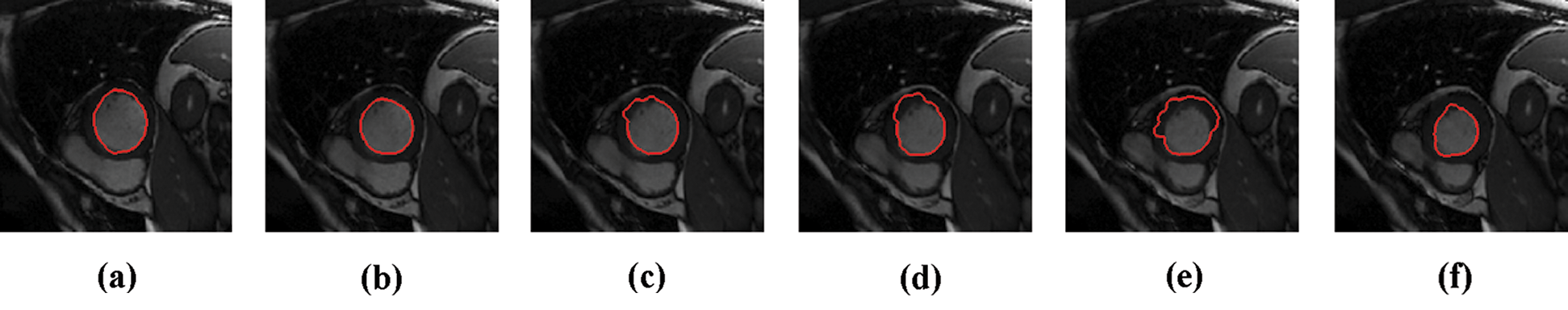
Figure 1: Sample results of Caselles technique

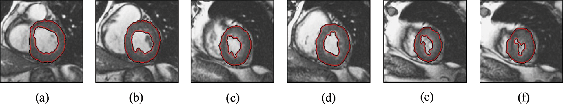
Figure 2: Sample results of Li technique

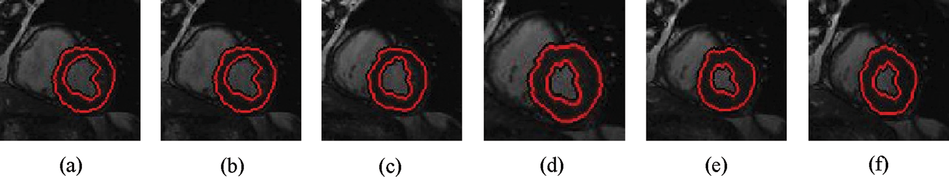
Figure 3: Sample results of Bernard-Friboulet technique

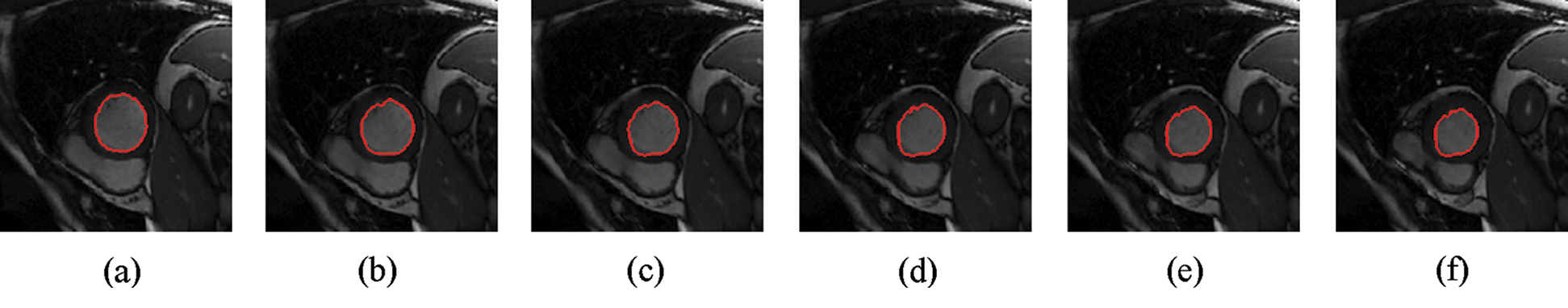
Figure 4: Sample results of Chan-Vese technique

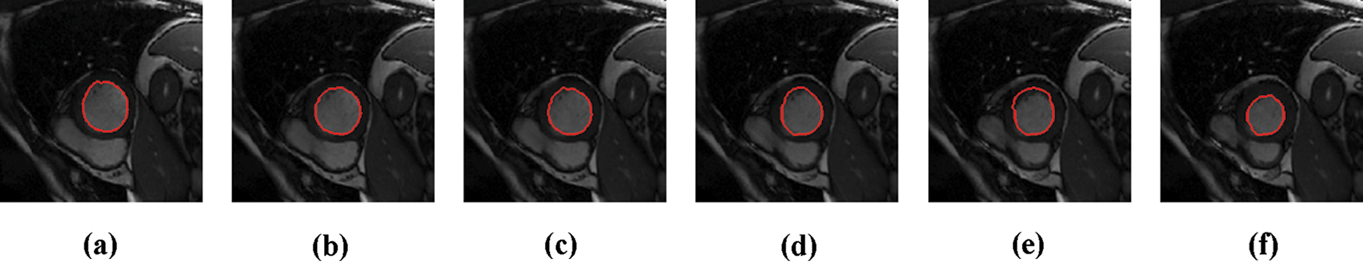
Figure 5: Sample results of Lankton technique

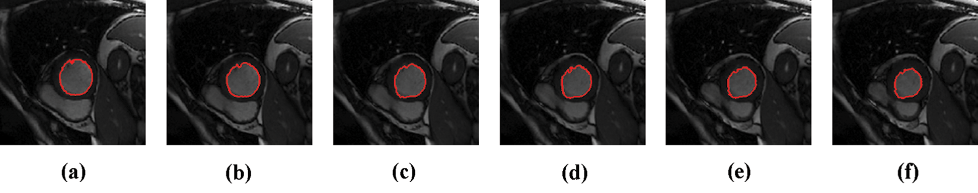
Figure 6: Sample results of Shi-Karl technique

6  Comparative Results

This section compares the performance of the studied medical image segmentation techniques. The segmentation quality is measured through comparing the resulted slices of different schemes with manual segmented slices using DM, PSNR, HS, and the execution time. The key performance matrices mean values of LV segmentation techniques are given in Tab. 1. Caselles, Chan-Vese and Shi-Karl techniques can successfully segmented the CMR slices. Also, Lankton technique gives good DM results, but it consumes much time to get closer to the object borders. Bernard and Li wideband segmentation techniques can’t give good results for segmenting LV blood pool.

The summery of the obtained results is explained in Tab. 2 that show the overall cardiac segmentation results in diastole and systole phases of the cardiac cycle of the heart. Most LV segmentation of CMR slices in the diastolic phase gives results better than the systolic phase results.

Shi-Karl and Chan-Vese techniques give good results in term of both the DM and computation time, but they don’t take the characteristics of the edges in consideration. Although the Shi-Karl technique gives better results in the equality values, the final outline of the Chan-Wes technique seems smooth due to the decryption of the level playing function used in the Shi-Karl technique. The DM column in Tab. 2 compares the DM values for all of the examined segmentation techniques. From that column, it’s clear to see that Shi-Karl and Chan-Vese techniques have highest and close values of DM measurements while the lowest similarity value is obtained by Bernard-Friboulet technique. The quality of the segmentation for all the examined techniques is measured using PSNR as shown in Tab. 2, PSNR column. In this column, the PSNR values for all of the examined segmentation techniques are compared. From that column, it’s easy to note that Shi-Karl and Chan-Vese techniques have highest and close values of PSNR measurements while the lowest value is obtained by Bernard-Friboulet technique. The next column in Tab. 2 entitled HS compares the HS values for all of the examined segmentation techniques. The lowest and close HS measurements are obtained using both of the Shi-Karl and Chan-Vese segmentation techniques while Bernard-Friboulet and Li techniques have the highest values of HS measurements. So, the obtained results of cardiac segmentation using Bernard-Friboulet and Li segmentation techniques are not accurate, wideband, and far from the ground truth. One more final point to state is that, both of Shi-Karl and Chan-Vese techniques have the lowest and close segmentation time as listed in Tab. 2. In conclusion, based on the obtained results, one can notice that, compared to all of the examined segmentation techniques, Shi-Karl segmentation technique produce best quality segmentation to the LV blood pool, and also it takes the lowest segmentation time. To be fair, we must say that, the Chan-Vese technique occupies the second rank from the segmentation quality and segmentation time points of view. Its results are very close to Shi-Karl technique. According to these results, Shi-Karl and Chan-Vese are the best in between the tested segmentation techniques. On the other hand, the LV blood pool segmentation quality obtained by Li and Bernard segmentation techniques is the worst. Such techniques also consumes the longest segmentation time. Therefore, in the range of the tested data sets and the examined segmentation techniques, we can say that, Li and Bernard segmentation techniques cannot separate the LV cavity from other parts of the image.

Table 1: Average comparative results of segmentation on slices from the first, second, and third dataset using different techniques

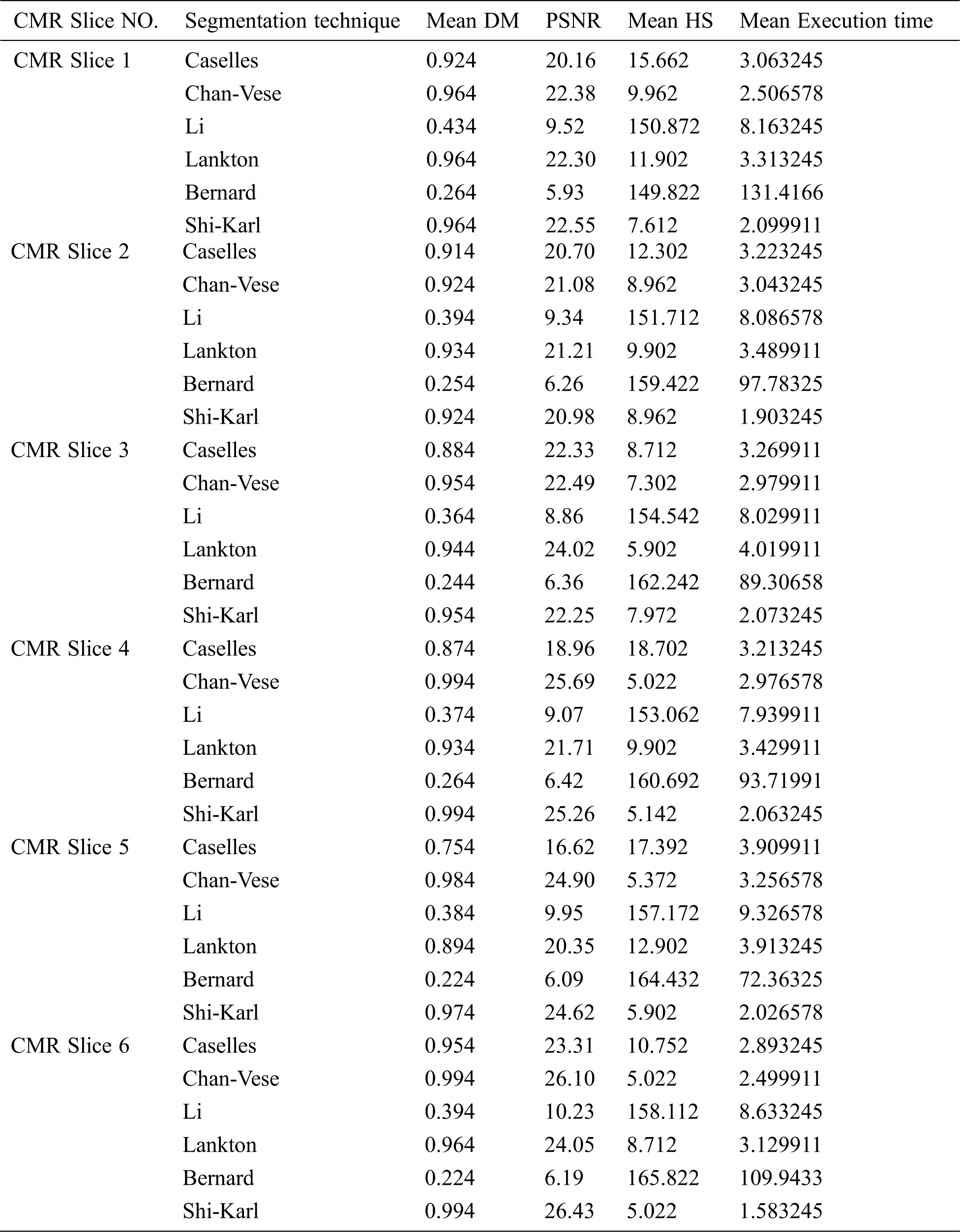
Table 2: Average comparative results of LV blood pool segmentation of CMR slices in systole phase and diastole phase

7  Conclusion

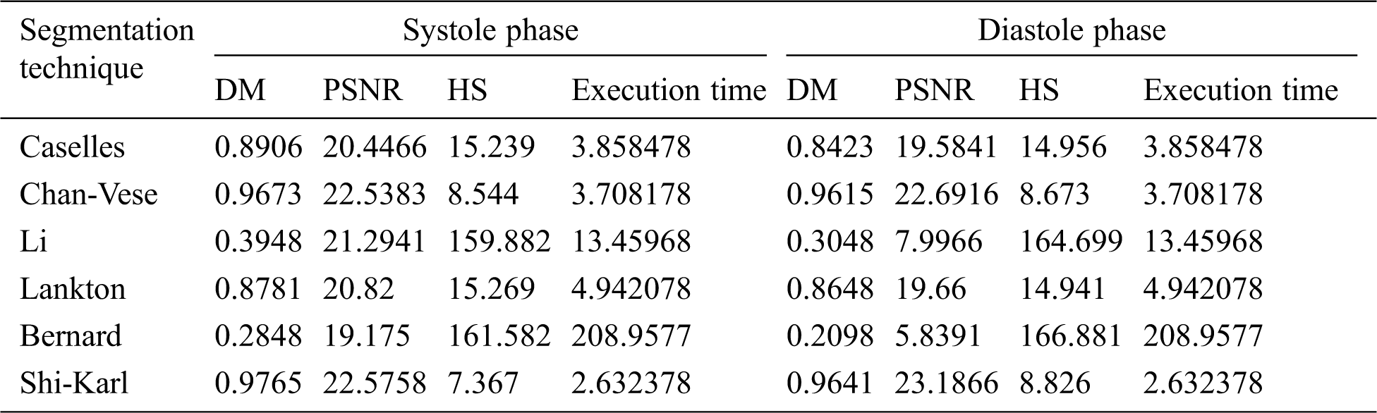
In this research paper, the performance of the studied segmentation techniques is evaluated and compared using a multi-axis 3D multi-layer CMRI dataset using several key performance indicators such as PSNR, DM, and HS. During the experiments, the same 3D short-axis multilayer CMR dataset is used for various case studies to illustrate the results of such segmentation techniques. In the range of the tested datasets and examined segmentation techniques, it is noticed that the Shi-Karl segmentation technique is the best due to the resulted segmentation quality and segmentation time points of view. The Chan-Vese technique occupies the second rank from the segmentation quality and segmentation time points of view. Its results are particularly close to the Shi-Karl technique results. However, LV blood pool segmentation quality obtained by the Li and Bernard segmentation techniques is the worst. Such techniques also consume the longest segmentation time. Therefore, in the range of the tested datasets and the examined segmentation techniques, we can state that the Li and Bernard segmentation techniques cannot separate the LV cavity from other parts of the image. According to these results, the Shi-Karl and Chan-Vese techniques are the optimal choice among the tested segmentation techniques in separating the LV cavity from other parts of the CMR images.

Acknowledgement: This study was funded by the Deanship of Scientific Research, Taif University Researchers Supporting Project number (TURSP-2020/08), Taif University, Taif, Saudi Arabia.

Funding Statement: This study was funded by the Deanship of Scientific Research, Taif University Researchers Supporting Project number (TURSP-2020/08), Taif University, Taif, Saudi Arabia.

Conflicts of Interest: The authors declare that they have no conflicts of interest to report regarding the present study.

This work is licensed under a Creative Commons Attribution 4.0 International License, which permits unrestricted use, distribution, and reproduction in any medium, provided the original work is properly cited.