Intelligent Automation & Soft Computing DOI:10.32604/iasc.2021.016981
Article

Adaptive Multi-Layer Selective Ensemble Least Square Support Vector Machines with Applications

Gang Yu1,4,5, Jian Tang2,*, Jian Zhang3 and Zhonghui Wang6

1State Key Laboratory of Process Automation in Mining & Metallurgy, Beijing, 102600, China
2Faculty of Information Technology, Beijing University of Technology, Beijing, 100024, China
3School of Computer and Software, Nanjing University of Information Science & Technology, 210044, China
4Beijing Key Laboratory of Process Automation in Mining & Metallurgy, Beijing, 102600, China
5BGRIMM Technology Group Co., Ltd., Beijing, 102600, China
6Department of Computer and Information Science, The University of Mississippi, Mississippi, MS 38655, USA
*Corresponding Author: Jian Tang. Email: freeflytang@bjut.edu.cn
Received: 17 January 2021; Accepted: 01 March 2021

Abstract: Kernel learning based on structure risk minimum can be employed to build a soft measuring model for analyzing small samples. However, it is difficult to select learning parameters, such as kernel parameter (KP) and regularization parameter (RP). In this paper, a soft measuring method is investigated to select learning parameters, which is based on adaptive multi-layer selective ensemble (AMLSEN) and least-square support vector machine (LSSVM). First, candidate kernels and RPs with K and R numbers are preset based on prior knowledge, and candidate sub-sub-models with K*R numbers are constructed through utilizing LSSVM. Second, the candidate sub-sub-models with same KPs and different RPs are selectively fused by using the branch and bound SEN (BBSEN) to obtain K SEN-sub-models. Third, these SEN-sub-models are selectively combined through using BBSEN again to obtain SEN models with different ensemble sizes, and then a new metric index is defined to determine the final AMLSEN-LSSVM-based soft measuring model. Finally, the learning parameters and ensemble sizes of different SEN layers are obtained adaptively. Simulation results based on the UCI benchmark and practical DXN datasets are conducted to validate the effectiveness of the proposed approach.

Keywords: Multi-layer selective ensemble learning; least square support vector machine; soft measuring model; municipal solid waste incineration; dioxins emission

1  Introduction

Data-driven soft measuring techniques can be used for online estimation of offline assay process parameters and experts’ estimation quantity variables [1,2]. Especially, soft measuring models are used in many fields according to their inferential estimation capability [3], and the two most common ones include artificial neural networks (ANN) and support vector machines (SVM). Although ANN is used to model DXN emission concentration [4], it has several shortcomings, such as easily falling into local minimum, over fitting, and unstable generalization performance in terms of small samples. For SVM, it is more suitable to build a prediction model for DXN emission, however, its prediction performance heavily depends on kernel and RPs [5]. Furthermore, SVM has to suffer from the quadratic program (QP) problem, which can be solved by least square-support vector machines (LSSVMs) including a set of linear equations. Due to the data dependence of kernel learning methods [6], some optimization methods are employed to address this problem through using single- or multi-objective optimization in terms of learning parameters [7,8]. However, such methods are time-consumed and prone to obtain a sub-optimum solution [9]. In addition, as the KP determines the geometry of the feature space, it can be optimally selected through class reparability [10,11]. Thus, this parameter is also calculated by using Fisher discrimination of classification problems [12]. For regression problems, a stable generalization performance can only be found within a certain range. However, the evaluation process must be dynamic and the searching results are unstable for small samples. Therefore, a fast and definitive method for KP selection should be developed in future researches. The RP of kernel learning method has no intuitive meaning in terms of geometry and is normally determined through cross-validation or optimization search methods [13]. In Wang et al. [14], a KP selection approach is proposed for small high-dimensional mechanical frequency spectral samples, which only selects a single kernel. Moreover, multiple kernel learning algorithms exhibit high efficiency and effectiveness in both classification and regression tasks [14]. And one of them named multiple kernel ensemble learning approach has been applied into hyper-spectral remote sensing image classification [15,16]. However, the optimized selection of learning parameters is not addressed jointly. Therefore, a new adaptive method for selecting learning parameters should be developed to model small samples with complex characteristics.

Selective ensemble (SEN) modeling can selectively fuse multiple sub-models in a linear or nonlinear method and achieve better prediction performances than single modeling. However, SEN modeling still exerts several limitations. One of them is ensemble construction, which creates a set of candidate sub-models for the same training dataset. The ensemble construction method based on the resample of training samples validates the ensemble method, and many available sub-models can obtain better performances than the ensemble of all the sub-models [17]. However, the selection problem of learning parameters remains unsolved in this scenario. Consequently, based on the above ensemble construction strategy, double-layer GA-based SEN latent structure modeling is proposed for collinear and nonlinear data [18]. However, this method has disadvantages of long searching time and randomized prediction results. Another ensemble construction method named manipulation of input features is used to model multi-source multi-scale high-dimensional frequency spectral data [13,19,20], and it can construct a soft measuring model by using the interesting mechanical sub-signals and their spectral feature subsets, which focuses on the selective fusion of different multi-source feature sub-sets from the perspective of selective information fusion. As a result, this method is thus suitable for modeling frequency spectral data with multi-source and high dimension, especially for small samples.

In this paper, the SEN kernel leaning algorithm for small data-driven samples is adopted to softly measure the DXN emission. Although several SEN-LSSVMs such as fuzzy C-means cluster-based SEN-LSSVM [21] and evolutionary programming (EP)-based multi-level LSSVM [22] have been proposed, they do not address the selection problem of learning parameters and are unsuitable for small samples. As multiple KPs can clearly describe the complex characteristics of small sample data (e.g., DXN), a soft measuring model for the SEN-LSSVM-based DXN emission concentration can be built through using multiple candidate KPs and the ensemble construction strategy. Meanwhile, the RP of the kernel learning algorithm is also data-dependent. Therefore, the algorithm can also be used and selected with the same idea like KPs.

Motivated by the above problems, this paper proposes a new adaptive multi-layer SEN-LSSVM (AMLSEN-LSSVM) method for modeling small samples with complex characteristics. Compared to the existing literatures, the distinctive contributions of this study are listed as follows. (1) A new SEN-LSSVM modeling framework is proposed to model small samples according to the candidate learning parameters at the first time; (2) The proposed method can adaptively select the kernel and RPs simultaneously. Moreover, the ensemble sizes of different SEN layers are also adaptively determined in implicit pattern; (3) A new metric index is defined for selecting the final AMLSEN-LSSVM soft measuring model to achieve tradeoff between model complexity and prediction performance.

The remainder of this paper is organized as follows. Section 2 describes the proposed modeling strategy. In Section 3, a detailed realization of the proposed approach is demonstrated. Section 4 presents the experimental results on two UCI benchmarks and practical DXN datasets for references. Finally, Section 5 concludes this paper.

2  Modeling Strategy Description

Based on the above analysis, an adaptive multi-layer SEN-LSSVM (AMLSEN-LSSVM) soft measuring strategy is proposed, which consists of candidate sub-sub-models, candidate SEN-sub-models, SEN-models, and decision selection modules. The process is shown in Fig. 1.

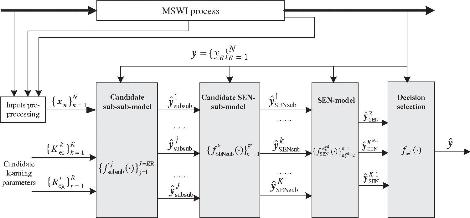
Figure 1: SEN-LSSVM-based soft measuring strategy

In Fig. 1, X={xn}n=1N is the input of the modeling data with features from the different phases of the MSWI process; y={yn}n=1N denotes the predicted data of the offline assay process; {Kerk}k=1K and {Regr}r=1R are the K candidate kernels and the R RPs, respectively; {fsubsubj(⋅)}j=1J=KR indicates the K × R candidate sub-sub-models set; y^subsubj is the prediction output of the jth sub-sub-model fsubsubj(⋅) ; {fSENsubk(⋅)}k=1K is the K candidate SEN-sub-model sets; y^SENsubk is the prediction output of the kth SEN-sub-model fSENsubk(⋅) ; {fSENKksel(⋅)}Kksel=2K−1 is the set of candidate SEN models; y^SENKsel is the prediction output of the SEN model with an ensemble sizeKsel ; fsel(⋅) and y^ are the final SEN soft sensor model and its prediction output, respectively.

The functions of the different modules are illustrated as follows:

(1) Candidate sub-sub-model module: Construct the K×R LSSVM sub-sub-models by using different candidate learning parameters.

(2) Candidate SEN-sub-model module: Construct the K SEN-sub-models by using the prediction outputs of R sub-sub-models based on the same KP and R different RPs.

(3) SEN-model module: Construct the SEN-models with an ensemble size from 2 to (K – 1) by using the prediction outputs of K SEN-sub-models based on different KPs.

(4) Decision selection module: Select the final soft measuring model from SEN-models with the different ensemble sizes by defining a new metric index and making a trade-off between prediction accuracy and model complexity.

3  Modeling Realization

3.1 Candidate Sub-Sub-Model Module

As the candidate kernels and RPs of the LSSVM model are respectively denoted as {Kerk}k=1K and {Regr}r=1R , the candidate learning parameters can be used to obtain the following matrix:

Mpara=[[Ker1,Reg1]⋯[Ker1,Regr]⋯[Ker1,RegR]⋮⋮⋮⋮⋮[Kerk,Reg1]⋯[Kerk,Regr]⋯[Kerk,RegR]⋮⋮⋮⋮⋮[KerK,Reg1]⋯[KerK,Regr]⋯[KerK,RegR]]J (1)

where [Kerk,Regr] is the jth element of learning parameter matrix Mpara , in which Mparaj=[Kerk,Regr] with j=1,⋯,J . Especially, J=K×R is the element number of matrix Mpara , that is, the number of LSSVM sub-sub-models.

Taken the jth pair [Kerk,Regr] of learning parameters for an example, the process of the sub-sub-model is built as follows. First, nonlinear mapping function φ(xn) is used to map {xn}n=1N into a higher dimensional feature space. Then, the optimization problem is solved by the LSSVM algorithm:

{minWj,bj⁡OjLS−SVM=12wjTwj+12Reg∑n=1Nζjn2s.t:y^jn=wjTφ(xnj)+bj+ζjn (2)

where wj is the weighted coefficient, bj indicates the bias, and ζjn denotes the prediction error of the nth sample. Thus, the Lagrange method can be employed to solve the optimization problem (2),

Lj(wj,bj,ζj,βj)=12wjTwj+12∑n=1N(ζjn)2−∑n=1Nβjn[wjTφ(xjn)+bj+ζjn−y^jn] (3)

where βj=[βj1,⋯,βjn,⋯,βjN] is the Lagrange operator vector, and ζj=[ζj1,⋯,ζjn,⋯,ζjN] is the prediction error vector. Taken the derivation of the parameters in Eq. (3), the optimum solution can be gotten by

∂Lj∂wj=0,∂Lj∂bj=0,∂Lj∂ξj=0,∂Lj∂βj=0, (4)

Ωkerj(x,xn)=<φ(x)⋅φ(xn)>=fkerj(x,xn,Kker), (5)

where Ωkerk(⋅) is the kernel function with parameter Kerk .

Accordingly, the above problem becomes a linear equation system:

[01⋯11fkerj(x1,x1,Kker),+1Regr⋯fkerj(x1,xN1,Kker)⋮⋮⋮⋮1fkerj(xN,x1,Kker)⋯fkerj(xN,xN,Kker)+1Regr]⋅[bjβj1⋮βjN]=[1y1⋮yN] (6)

By solving the above system, βj and bj are obtained. Then, the LSSVM sub-sub-model can be denoted as

y^subsubj=∑n=1Nβjn⋅Ωkerj(x,xn)+bj (7)

For a concise expression, (7) can also be expressed as

y^subsubj=fsubsubj(x;Mparaj)=fsubsubj(xj;Kerk,Regr)=fsubsubk,r(⋅) (8)

Therefore, all these candidate sub-sub-models are denoted as {fsubsubj(⋅)}j=1J , and the prediction outputs are {y^subsubj}j=1J .

3.2 Candidate SEN-Sub-Model Module

The prediction outputs of these candidate sub-sub-models can be rewritten as

{y^subsubj}j=1J={ysubsub1,1,⋯,ysubsub1,r,⋯,ysubsub1,R,⋮ysubsubk,1,⋯,ysubsubk,r,⋯,ysubsubk,R,⋮ysubsubK,1,⋯,ysubsubK,r,⋯,ysubsubK,R} (9)

where y^subsub1=fsubsub1,1(⋅) , y^subsubj=fsubsubk,r(⋅) , y^subsubJ=fsubsubK,R(⋅) .

In (9), the kth row contains all the sub-sub-models with the same Kerk and different {Regr}r=1R . Thus, {y^subsubj}j=1J can be rewritten as

{y^subsubj}j=1J={{fsubsub1,r(⋅)}r=1R,⋮{fsubsubk,r(⋅)}r=1R,⋮{fsubsubK,r(⋅)}r=1R} (10)

The candidate SEN-sub-models are built for each row of (10) by selecting and combining the candidate sub-sub-models based on different {Regr}r=1R . For example, the kth row {fsubsubk,r(⋅)}r=1R can construct the kth SEN-sub-model fSENsubk(⋅) through the same Kerk and {Regr}r=1R . So the prediction output (y^SENsubk)n of the nth modeling sample can be calculated by

(y^SENsubk)n=fSENsubk(⋅)=∑rksel=1Rkselwrkselsel⋅(y^rkseln)sel=∑rksel=1Rkselwrkselsel⋅fsubsubk,rksel(xn,Kerk,Regrksel) (11)

where fsubsubk,rksel(⋅) , Regrksel , and (y^rksell)sel are the selected rkselth sub-sub-model, its RP, and the prediction output of the nth modeling sample, respectively; Rksel indicates the ensemble size, and wrkselsel is the weighted coefficient of the selected sub-sub-models, which is calculated by

wrkselsel=1σrksel2∑rksel=1Rksel1σrksel2 (12)

where σrksel is the standard variance of the prediction outputs {(y^rkseln)sel}n=1N form the selected rkselth sub-sub-model. As the ensemble size Rksel and the weighted algorithm are pre-set and determined, the ensemble sub-sub-models for constructing the kth SEN-sub-model fSENsubk(⋅) can be obtained by solving the following optimization problem:

(y^SENsubk)n=∑rksel=1Rkselwrkselsel⋅(y^rkseln)sel=∑rksel=1Rkselwrkselsel⋅fsubsubk,rksel(zn,Kerk,Regrksel)s.t.{min{{RMSE((y^SENsubk,)Rksel)}Rksel=2R}RMSE((y^SENsubk,)Rksel)=1N∑n=1N(yn−∑rksel=1Rkselwrkselsel⋅fsubsubk,rksel(zn,Kerk,Regrksel))22≤Rksel≤R,∑rksel=1Rkselwrkselsel=1,0<wrkselsel<1{fsubsubk,rksel}rksel=1Rksel∈{fsubsubk,r(⋅)}r=1R{Regrksel}rksel=1Rksel∈{Regr}r=1R (13)

where the root mean square error (RMSE) is used to evaluate the generalization performance of the SEN-sub-model with ensemble size Rksel .

In order to solve the above problem, the optimized ensemble sub-sub-models and their weighted coefficients are obtained through repeating the BBSEN optimization algorithm R−2 times [11], and this process is expressed by

{{fsubsubk,r(x;Kerk,Regr)}r=1R,{yn}n=1N}=fBBSEN({fsubsubk,rksel(x,Kerk,Regrksel)}rksel=1Rksel,{wrkselsel}r=1Rksel) (14)

where {fsubsubk,r(⋅)}k=1Kksel and {wsubsubk,r}k=1Kksel are the selected ensemble sub-sub-models and their weighted coefficients, respectively; and Rksel is the number of the selected sub-sub-models.

For simplification, all the RPs of the kth SEN-sub-model are denoted as (Regk)SENsub={Regrksel}rksel=1Rksel . After repeating the above modeling procedure K times, all the SEN-sub-models with KPs {Kerk}k=1K are obtained. And then these candidate SEN-sub-models and their prediction outputs can be denoted as {fSENsubk(⋅)}k=1K and {y^SENsubk}k=1K , respectively. Therefore, different RPs are adaptively selected in the construction process of these SEN-sub-models.

3.3 SEN-Model Module

Based on the above sub-sections, the SEN-sub-models with the same KPs and different RPs are obtained. Then, Equation (10) can be transformed into the following form.

{y^subsubj}j=1J={{fsubsub1,r(⋅)}r=1R,⋮{fsubsubk,r(⋅)}r=1R,⋮{fsubsubK,r(⋅)}r=1R}⇒⇒{{fsubsub1,r1sel(⋅)}r1sel=1R1sel,⋮{fsubsubk,rksel(⋅)}rksel=1Rksel,⋮{fsubsubK,rKsel(⋅)}rKsel=1RKsel,}={fSENsub1(⋅),⋮fSENsubk(⋅),⋮fSENsubK(⋅),}={fSENsubk(⋅)}k=1K={y^SENsubk}k=1K (15)

In this context, BBSEN is further employed to obtain the prediction output y^SENksel of SEN-model fSENsubksel(⋅) by optimally selecting and combining SEN-sub-models based on KPs{Kerk}k=1K . Hence, the optimization description is presented as

y^SENn=∑ksel=1KselwkselSENsel⋅(y^SENksel)n=wkselSENsel⋅fSENsubksel(⋅).t.{ RMSE(y^SENKsel)=1N∑n=1N(yn−∑ksel=1KselwkselSENsel⋅(y^SENksel)n)2=1N∑n=1N(yn−∑ksel=1KselwkselSENsel⋅fSENsubksel(zn,Kerksel,(Regksel)SENsub))22≤Ksel≤K,∑ksel=1KselwkselSENsel=1,0<wkselSENsel<1{fSENsubksel}ksel=1Ksel∈{fSENsubk(⋅)}k=1K{Kegksel}ksel=1Ksel∈{Kegr}r=1K (16)

where (Regksel)SENsub is the RP set for constructing the kselth SEN-sub model with size RSENsubksel ; Ksel indicates the number of selected ensemble SEN-sub-models (ensemble size) for building the SEN-model; fSENsubksel(⋅) and Kegksel represent the kselth ensemble SEN-sub-model and its KP, respectively; y^SENKsel denotes the prediction outputs of the nth samples of the SEN-model with ensemble size Ksel ; and wkselSENsel is the weighted coefficient of the kselth ensemble SEN-sub-model, which is calculated by

wkselSENsel=1σksel2∑ksel=1Ksel1σksel2 (17)

where σkksel is the standard variance of the prediction outputs {(y^SENksel)n}n=1N based on the selected kselth ensemble SEN-sub model. Consequentially, the above modeling process can be represented by

{fSENsubk(x,Kerk,(Regk)SENsub)}k=1K{yn}n=1N}⟶BBSEN{{fSENsubksel(x,Kerksel,(Regksel)SENsub)}ksel=1Ksel{wkselSENsel}ksel=1Ksel (18)

where {fSENsubksel(⋅)}ksel=1Ksel and {wSENsubksel}ksel=1Kksel are the selected ensemble SEN-sub-models and their weighted coefficients, respectively; and Kksel is the number of selected SEN-sub-models.

Accordingly, the SEN model fSENKksel(⋅) with ensemble size Kksel can be denoted as

y^SENKsel=∑ksel=1KselwkselSENsel⋅fSENsubksel(⋅)=∑ksel=1KselwkselSENsel⋅(∑rksel=1Rkselwrkselsel⋅fsubsubk,rksel(z,Kerksel,Regrksel))ksel (19)

In Eq. (19), the SEN-model fSENKsel(⋅) selects both the kernel and RPs adaptively from the candidates. Moreover, the ensemble size of SEN-sub-model is also decided adaptively in the SEN modeling process.

3.4 Decision Selection Module

Supposed that Kksel∈[2,K) is hold, and then (K−2) SEN models can be constructed. However, the complexity of the SEN model significantly increases with the ensemble size. In order to solve this problem, the model complexity in this paper is measured by the number of single LSSVM models. Thus, the complexity of the best sub-sub-model, the kth SEN-sub-model fSENsubk(⋅) , and the SEN model fSENKsel(⋅) are 1, Rksel , and ∑ksel=1KselRSENsubksel , respectively. To make a tradeoff between prediction accuracy and model complexity, the metric index for selecting the suitable soft sensor model is defined by

ξSENKsel=λRMSE(fSENKsel(⋅))∑Ksel=2K−1RMSE(fSENKsel(⋅))+(1−λ)∑ksel=1KselRSENsubksel∑Ksel=2K−1∑ksel=1KselRSENsubksel (20)

where λ is the coefficient between 0 and 1.

According to the above metric index, the SEN-model with the lowest RMSE is selected as the final DXN soft measuring model. Thus, the final prediction output is obtained by

y^=fsel(y^SEN2,⋯,y^SENKsel,⋯,y^SENK−1)s.t.min{ξSEN2,⋯,ξSENKsel,⋯,ξSENK−1} (21)

where fsel(⋅) represents the final AMLSEN-LSSVM model. In this way, the learning parameters and ensemble sizes of different SEN layers are selected adaptively.

4  Application Study

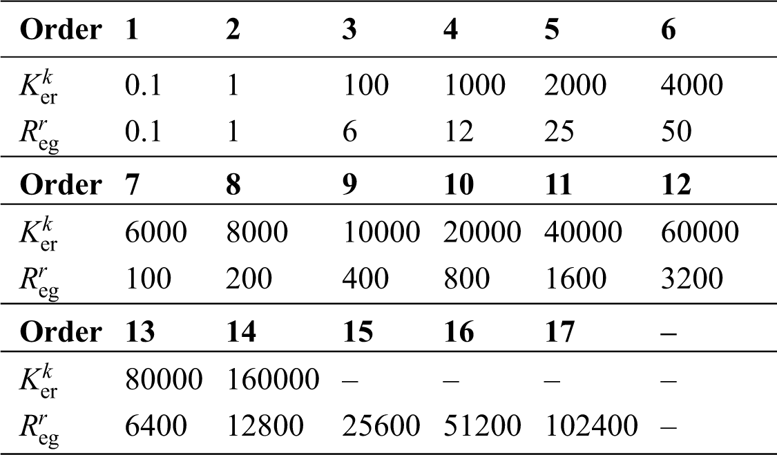
In this section, two UCI benchmarks and a practical DXN datasets are exploited to validate the proposed methods. Primarily, each dataset is divided into two parts: training data and testing data. Then radius basis function (RBF) is used for the kernel type of the LSSVM. Finally, the candidate kernel and RP datasets are selected as Can_1{0.1, 1, 100, 1000, 2000, 4000, 6000, 8000, 10000, 20000, 40000, 60000, 80000, 160000} and Can_2{0.1, 1, 6, 12, 25, 50, 100, 200, 400, 800, 1600, 3200, 6400, 12800, 25600, 51200, 102400}, respectively. Seen from the samples, Can_1 and Can_2 illustrate that the candidate learning parameters have a wide range. The order number and their values are shown in Tab. 1.

Table 1: Order number and learning parameters value

4.1 Data Description

In order to present preliminary results, two UCI benchmark datasets, Boston housing and concrete compressive strength, are used to validate the proposed method, which are listed as follows.

For Boston housing data, the inputs include: (1) the per capita crime rate of the town (CRIM);(2) the proportion of residential land zoned over 25,000 sq. ft. (ZN); (3) the proportion of non-retail business acres per town (INDUS); (4) the Charles River dummy variables (CHAS); (5) the nitric oxide concentrations (NOX); (6) the average number of rooms per dwelling (RM); (7) the proportion of owner-occupied units built before 1940 (AGE); (8) the weighted distances to five employment centers of Boston (DIS); (9) the index of radial highway accessibility (RAD); (10) the full property tax rate per $10,000 (TAX); (11) the pupil–teacher ratio of the town (B); (12) the lower status of the population (LSTAT); and (13) the median value of owner-occupied homes per $1000 (MEDV). The output is the housing values of the suburbs of Boston with data size 506.

For concrete compressive strength data, the inputs include: (1) cement; (2) blast furnace slag; (3) fly ash; (4) water; (5) superplasticizer; (6) coarse aggregate; (7) fine aggregate of the various ingredients of concrete placement per cubic meter; and (8) conserved days. The output is concrete compressive strength with data size 1030.

4.2 Modeling Results

According to the candidate learning parameters, 14 × 17 = 238 sub-sub-models based on the LSSVM are constructed. Correspondingly, the BBSEN method is employed to build 14 SEN-sub-models. The statistical results are shown in Tab. 2.

Table 2: Statistical results of different SEN-sub-models for benchmark datasets

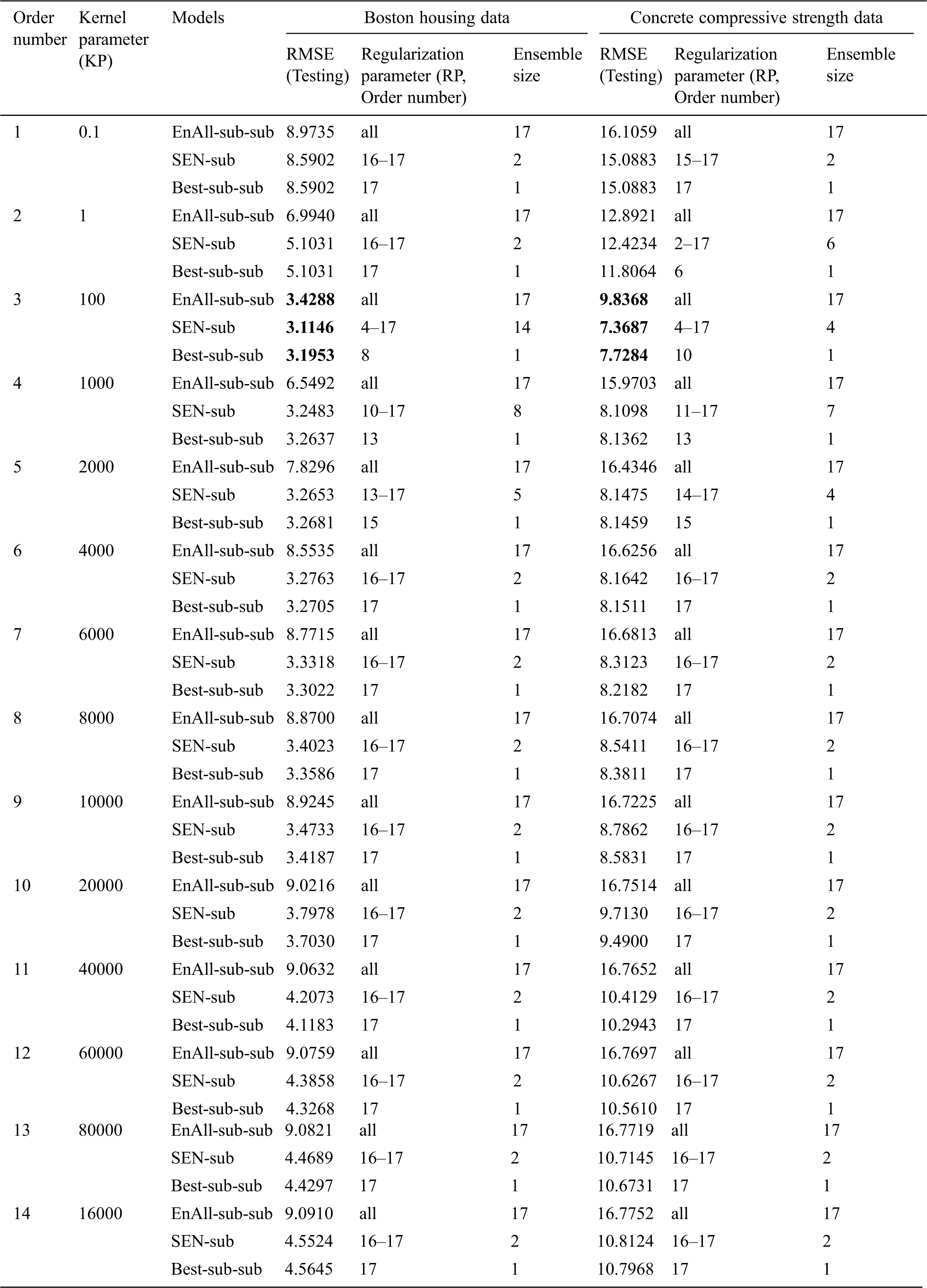
Tab. 2 illustrates that: (1) the best SEN-sub-model of Boston housing dataset has KP 100 and RPs {25, 50, 100, 200, 400, 800, 1600, 3200, 6400, 12800, 25600, 51200, 102400} with RMSE 3.1146 and an ensemble size 14. The best sub-sub-model picks up KP 100 and RP 200 with RMSE 3.1953, and the best EnAll-sub-sub-model possesses the same KP with RMSE 3.4288;(2) the best SEN-sub-model of concrete compressive strength data has the KP 100 and RPs {25, 50, 100, 200, 400, 800, 1600, 3200, 6400, 12800, 25600, 51200, 102400} with RMSE 7.368 and an ensemble size 14. The best sub-sub-model picks up KP 100 and RP 800 with RMSE 7.7284, and the best EnAll-sub-sub-model possesses the same KP with RMSE 9.8368;(3) different KPs have different effects on the prediction performance of the SEN-sub-models, so that parts of the best sub-sub-models have lower RMSEs than those of the SEN-sub-models. Thus, setting a suitable RP is very important to demonstrate the relationship among RMSEs, ensemble sizes, and different types of models with the single KP, which are shown in Figs. 2 and 3.

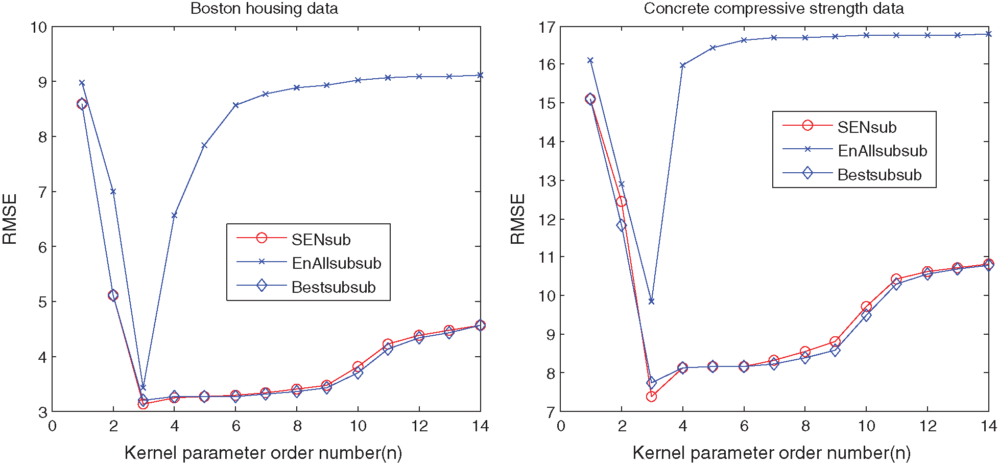
Figure 2: Relationship between RMSEs and different types of models based on the single KP for the UCI benchmark datasets

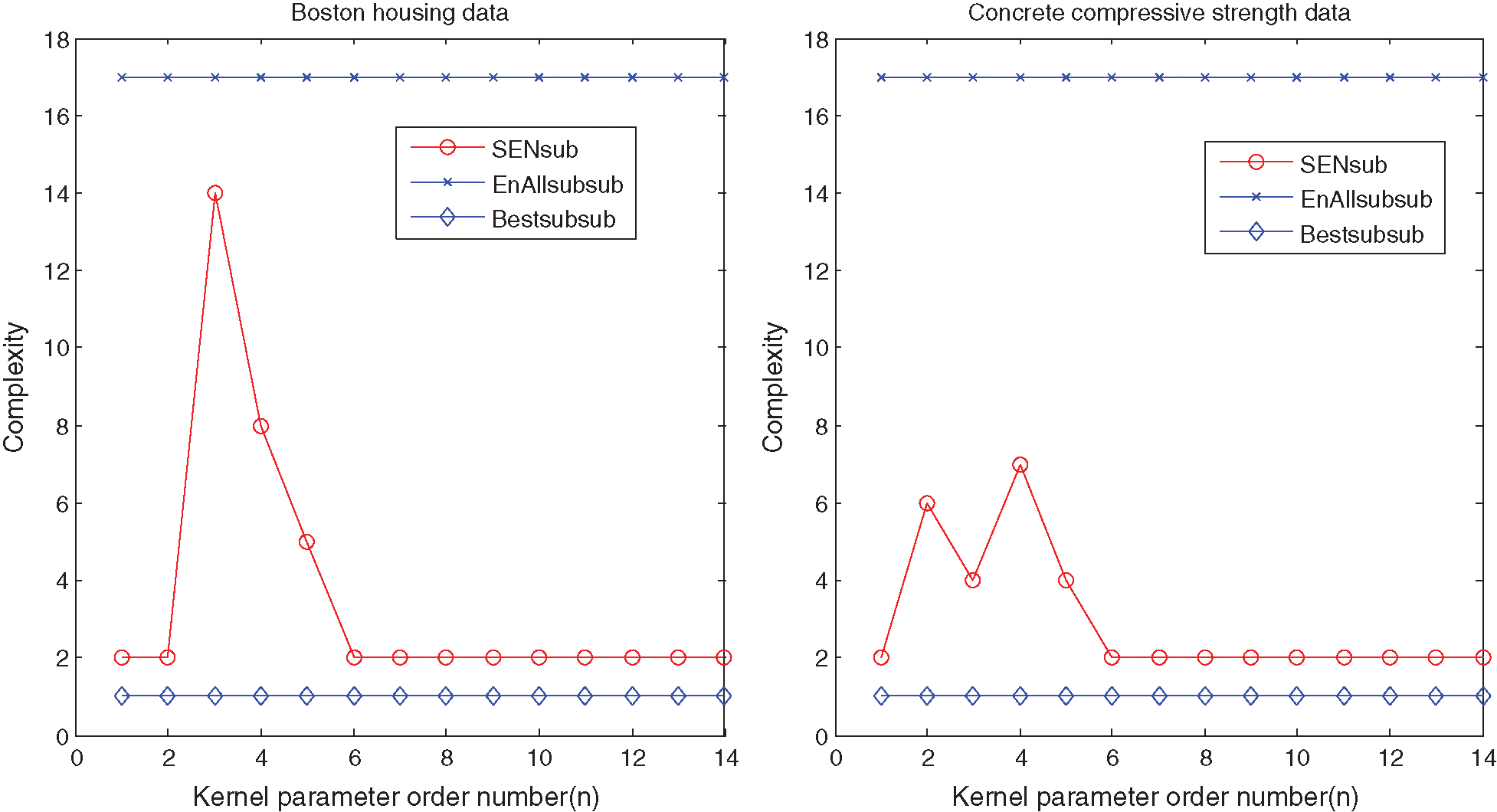
Figure 3: Relationships between ensemble sizes and different models based on the single KP for the UCI benchmark datasets

Figs. 2 and 3 show that suitable learning parameters are crucial. From this perspective, the ensemble size with the best prediction performance of the Housing and Concrete data are 14 and 6 in terms of the same KP 100, respectively. However, the ensemble size of the SEN-sub-model does not increase with the KPs after 4000.

For the 14 SEN-sub-models, the BBSEN method is used again to obtain the SEN-model with a different ensemble size, and the detailed statistical results of the SEN-models are illustrated in Tab. 3.

Table 3a: Statistical results of all SEN-models for the Boston housing dataset

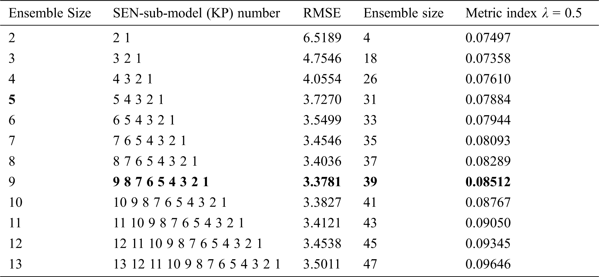
Table 3b: Statistical results of all SEN-models for the concrete compressive strength dataset

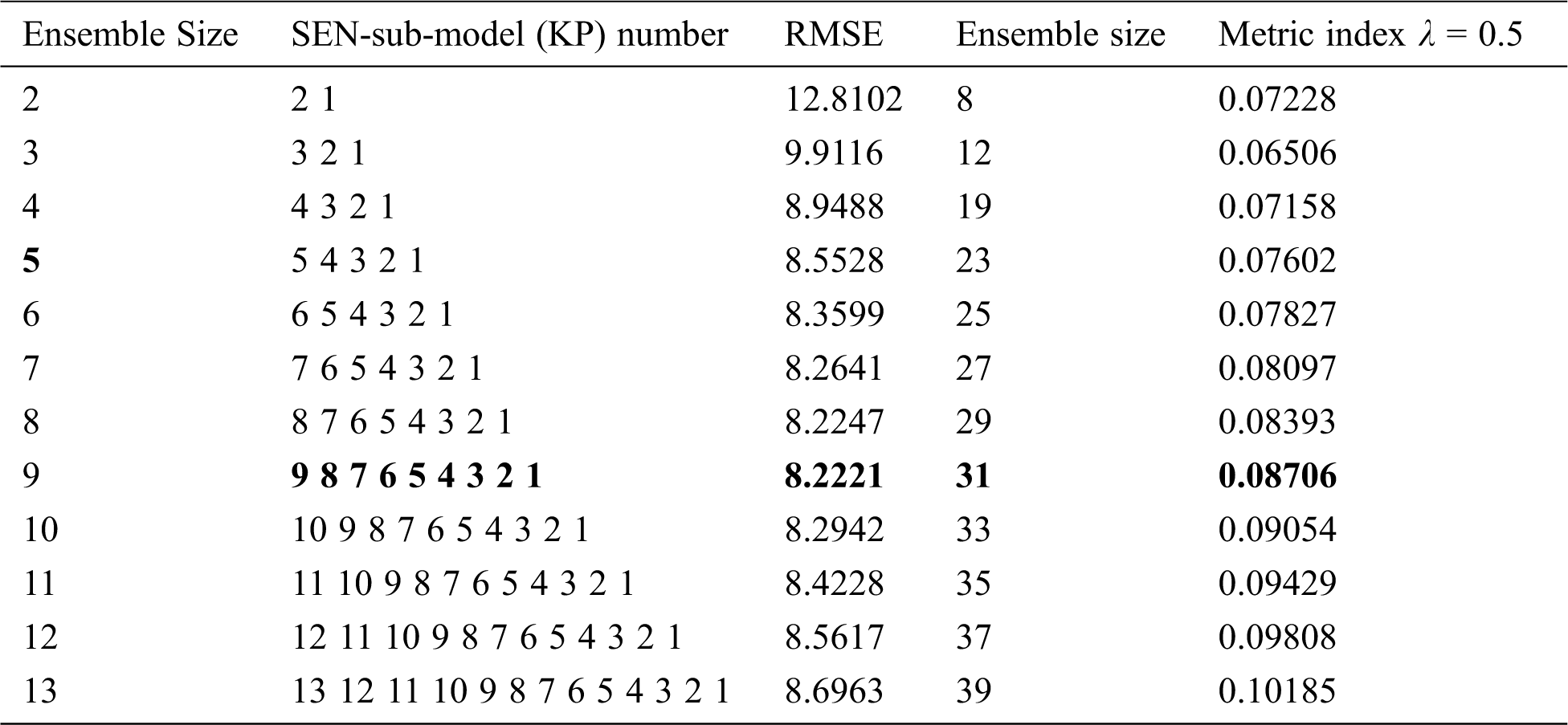
Tab. 3 shows that:(1) in the Boston housing dataset, the SEN-model with an ensemble size 9, KPs {0.1, 1, 100, 1000, 2000, 4000, 6000, 8000, 10000}, has the best prediction performance (RMSE 3.3781) among all the SEN-models, which is higher than that of the best SEN-sub-mode, but lower than that of the EnAll-SEN-sub-model;(2) in the concrete compressive strength dataset, the SEN-model with an ensemble size 9, KPs {0.1, 1, 100, 1000, 2000, 4000, 6000, 8000, 10000}, has the best prediction performance (RMSE 8.2221) among all the SEN-models. However, it is larger than that of the best SEN-sub-mode, but lower than that of the EnAll-SEN-sub-model; (3) the best SEN-sub-models in the above datasets has the best prediction performance. Moreover, the prediction performance of different SEN-models is not further improved with the increase of the ensemble size. The relationship between RMSEs and the ensemble sizes of SEN models is shown in Figs. 4 and 5.

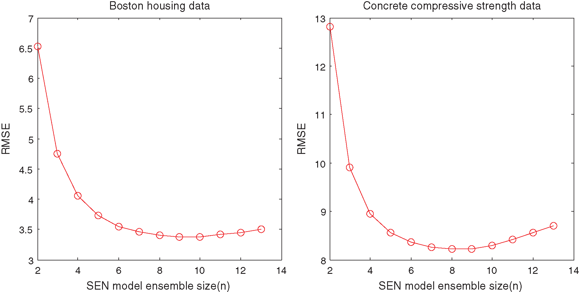
Figure 4: RMSE of SEN model with different ensemble sizes for the UCI benchmark datasets

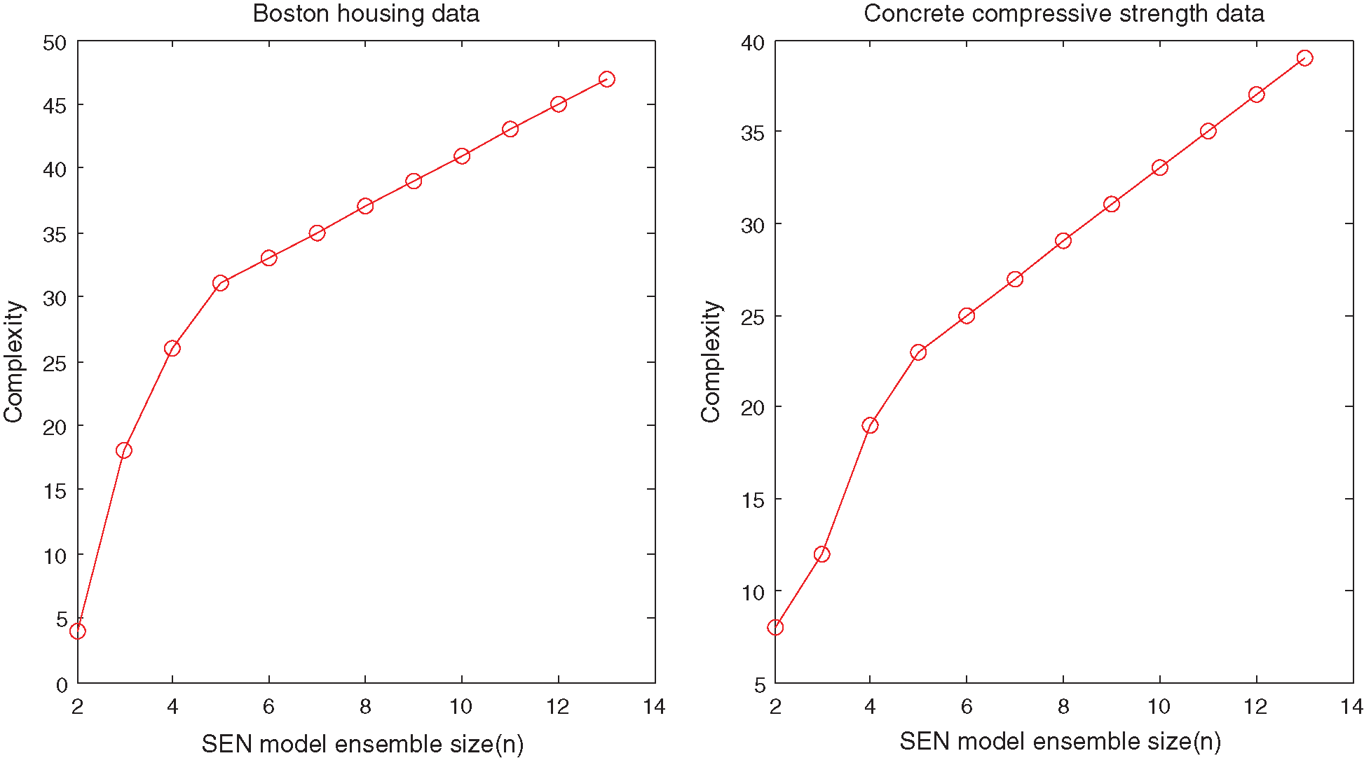
Figure 5: Ensemble size of SEN model with different ensemble sizes for the UCI benchmark datasets

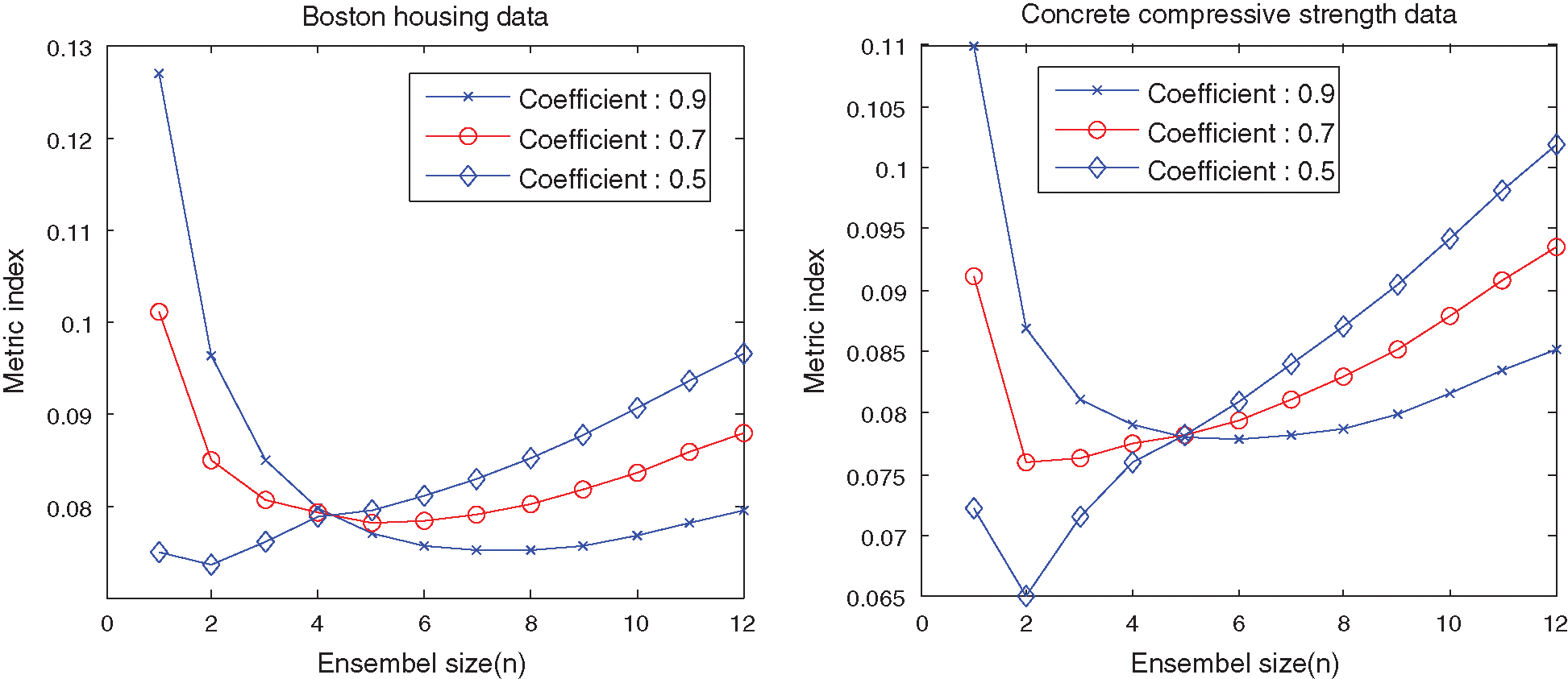
Figure 6: Metric index curves of the SEN-models with different λ values

The above results show that it is essential to make a tradeoff between prediction performance and model complexity. The proposed indices of different SEN-models with λ = 0.5 are shown in Tab. 3, and the metric index curves of the SEN-model with different λ values are shown in Fig. 6.

Seen form Fig. 6, the optimal value of the metric index shifts to the left with increasing coefficient (λ ) value. Thus, it can be determined by the practical requirement. The prediction curves of the best SEN-sub-model (SENsub) and the best SEN-model (SenSENsub) on the minimum prediction errors as well as the ensemble all SEN-sub-model (EnSENsub) are shown in Figs. 7 and 8, respectively.

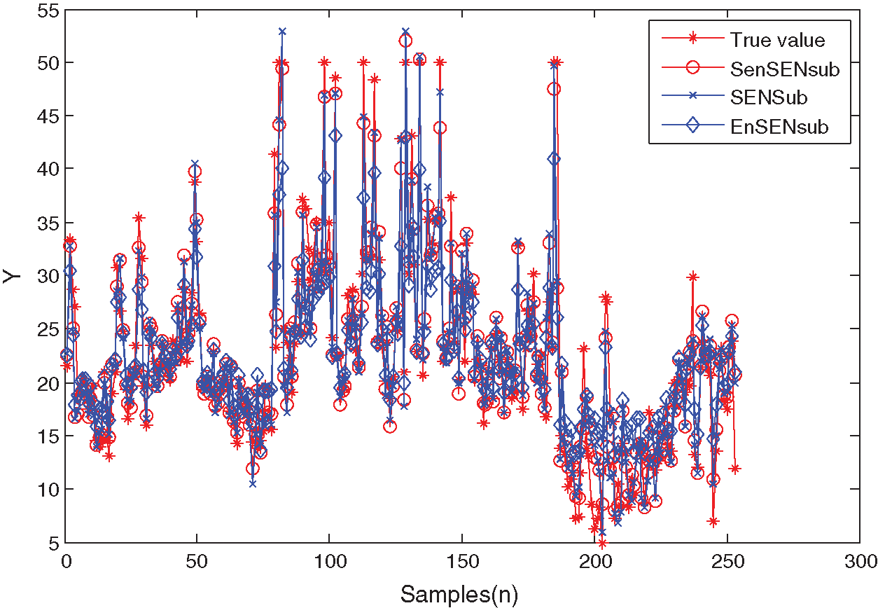
Figure 7: Prediction curves of the Boston housing data

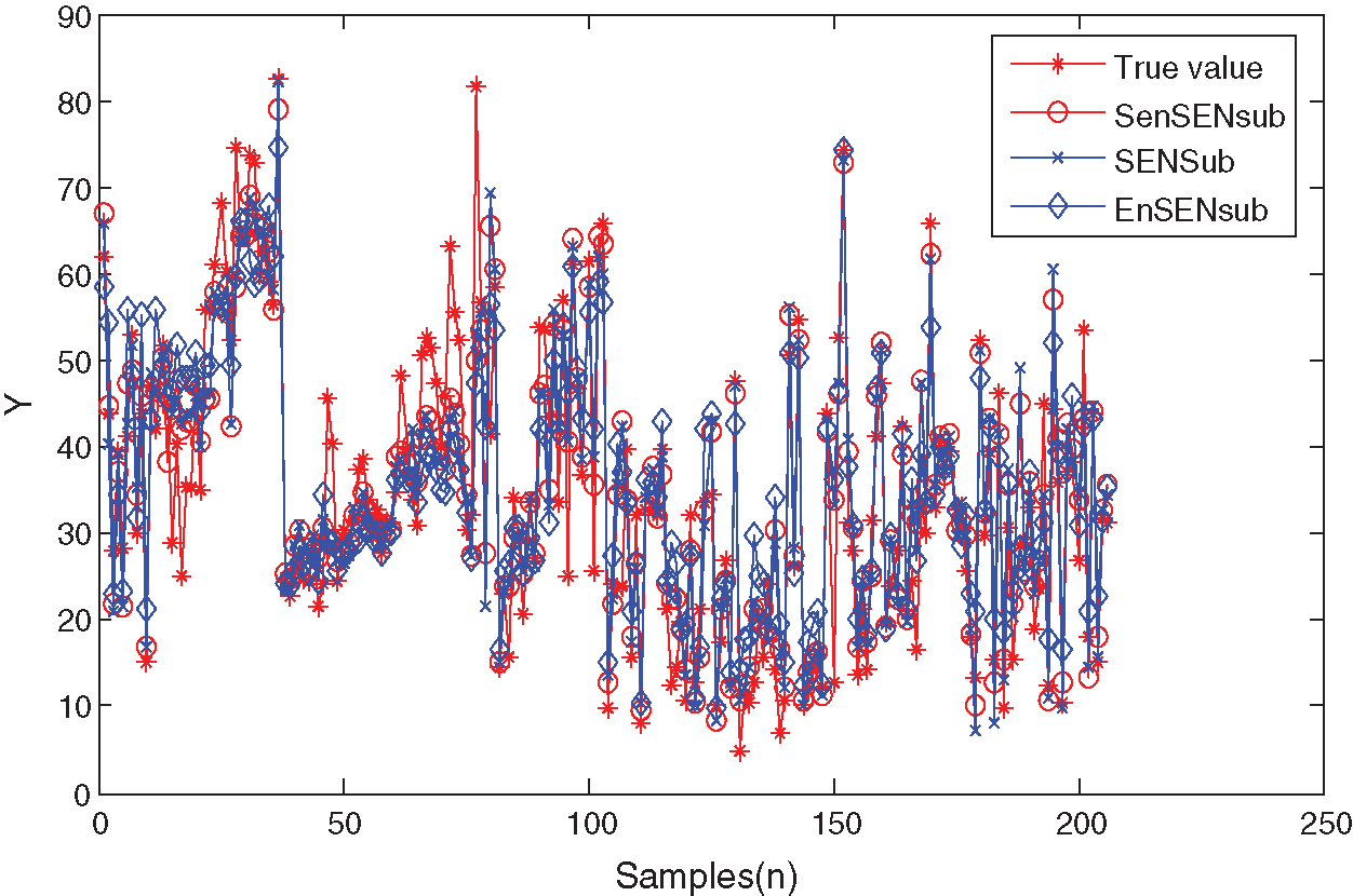
Figure 8: Prediction curves of the concrete compressive strength data

The above results show that the proposed method can model the two UCI benchmark datasets effectively, which can make an adaptive selection of the learning parameters.

4.3 Comparative Results

The proposed method is compared with the PLS, KPLS, GASEN-BPNN, and GASEN-LSSVM approaches. Concretely, the number of latent variables (LVs) and kernel LVs (KLVs) are decided by the leave-one-out cross-validation, and the number of hidden nodes of the GASEN-BPNN is set to two times plus one of the original inputs’ number. Thus, the structure of BPNN is 13-27-1 for the housing data, and 8-16-1 for concrete data. Meanwhile, the learning parameters of GASEN-LSSVM are used as ones of the best sub-sub-model in the proposed method. For GASEN-BPNN and GASEN-LSSVM, the modelling process is repeated 10 times to overcome their randomness.

Table 4: Statistical results of comparative methods

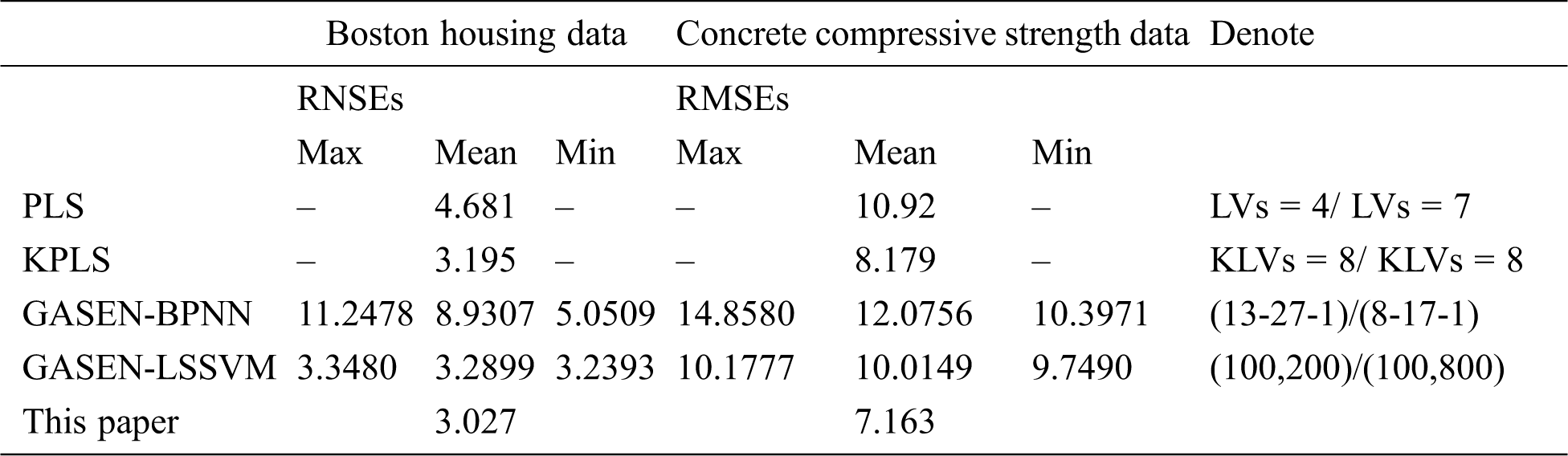
Tab. 4 shows that the proposed method has the best prediction performance without any disturbance.

Although the GASEN-based prediction results are disturbed within a certain range due to the random initialization of the input weights and the bias of BPNN and population GA, the PLS/KPLS methods can activate the extracted latent variables to construct a linear or nonlinear model with a single KP for stabilization.

4.4 Discussions

4.4.1 Kernel Parameter

KP determines the geometry of the feature space, which can be calculated by using the Fisher discrimination for classification problem. Actually, due to the deficiency of the range obtained for the regression problem, the candidate KP set in our proposed method serves as the key factor to obtain an effective soft sensor model. In addition, a wide range of KPs must be used for very small sample data with complex characteristics, such as DXN.

4.4.2 Regularization Parameter

RP is always decided by the cross validation or other optimization methods. In terms of results, a small number of modeling samples require more RPs, that is, the ensemble size increases with decrease of the number of samples. Moreover, a large KP requires a small number of RPs. As a result, the reasonable range should also be optimized in the future studies.

4.4.3 Ensemble Size

Selecting a suitable number of ensemble sub-models from candidates in the SEN-modeled process means that more ensemble sub-models leads to the more complex method, which implies sub-sub-models can measure the complexity of the proposed AMLSEN method. In practice, the ensemble size of the SEN-model in the proposed method is selected to make a trade-off between prediction accuracy and model complexity. Additionally, the ensemble size of the SEN-sub-model is implicitly determined by using the BBSEN algorithm in terms of prediction performance. Thus, the proposed method has a flexible structure to demonstrate the conclusion that the ensemble size increases with the decrease of the number of training samples.

5  Conclusions

A new soft measuring method is proposed based on the AMLSEN-LSSVM algorithm, and many sub-sub-models based on the different candidate learning parameters are constructed by using the LSSVM. According to the same KP, these candidate sub-sub-models are selectively fused to obtain SEN-sub-models by using the BBSEN, which are selectively combined by using the BBSEN again for building SEN models with different ensemble sizes. Ultimately, the final soft measuring model is determined based on a newly defined metric index. The simulation results based on the benchmark datasets show the effectiveness of the proposed method, which demonstrate that not only the proposed method can be used for softly measuring other difficult-to-measure process parameters in different industrial processes, but also a more common adaptive multi-layer SEN modeling framework can be explored.

Funding Statement: This research is supported by the State Key Laboratory of Process Automation in Mining & Metallurgy and Beijing Key Laboratory of Process Automation in Mining & Metallurgy under the Grant No. BGRIMM-KZSKL-2020-02, and National Key Research and Development Project under the Grant No. 2020YFE0201100 and 2019YFE0105000. The authors Jian Zhang and Jian Tang received the grants, respectively, and the URLs of sponsor’s website is https://www.bgrimm.com/.

Conflicts of Interest: The authors declare that they have no conflicts of interest to report regarding the present study.

This work is licensed under a Creative Commons Attribution 4.0 International License, which permits unrestricted use, distribution, and reproduction in any medium, provided the original work is properly cited.