DOI:10.32604/iasc.2021.016405
| Intelligent Automation & Soft Computing DOI:10.32604/iasc.2021.016405 | |
| Article |
Energy Aware Clustering with Multihop Routing Algorithm for Wireless Sensor Networks
School of Computing Science & Engineering, Galgotias University, Greater Noida, 203201, India
*Corresponding Author: A. Daniel. Email: danielarockiam@gmail.com
Received: 01 January 2021; Accepted: 24 March 2021
Abstract: The Internet of Things (IoT) and the Wireless Sensor Network (WSN) concepts are currently combined to improve data transmission based on sensors in near future applications. Since IoT devices exist in WSN with built-in batteries, power efficiency is a challenge that must be resolved. Clustering and routing are effectively treated as methods for reducing the dissipation of energy and maximising WSN IoT support life. This paper presents the new Energy Aware Adaptive Fuzzy neuro clustering with the WSN assisted IoT algorithm EAANFC-MR. EAANFC-MR is proposed for two main stages, clustering and multihop routing on the basis of EAANFCs. For selecting CHs with Residual Energy (RE) and Distance and Node degrees the EAANFC based cluster technique is used. The QOBFO algorithm, which is used as a Multihop Route Technique, is then used to select optimised roads to the destination. MATLAB is used to simulate the proposed EAANFC-MR model. The goodness of the EAANFC-MR model interspersed with various aspects was demonstrated through a series of experiments.
Keywords: IoT; sensor networks; clustering; energy efficiency; multihop routing
The use of the internet has progressively evolved in daily life in recent decades. The principal objective of a global networking environment such as an intelligent communication system is to connect all entities in the environment. The Internet of Things (IoT) is used in the interest of modern society and is composed almost by wireless sensor knots and networks. It combines people and things. This kind of innovation leads to the development, by physical and virtual utilities, of new models and services. The IoT concept relies on previous models of communication. It is therefore impossible and highly challenging to develop a substantial and essential IoT system according to the necessary factors. For each sensor device and object, the efficiency of IoT is important to ensure the latest interoperability. In comparison to the IoT platform, Wireless Sensor Network (WSN) [1] plays an essential role, particularly in developing integrated circuits to support modification of sensory sensing devices, to determine the weather conditions and to collect the relevant data transmitted to users on the platform. The life span of a battery that has to be considered when designing the model [2] is an important factor at this point. A node of the sensor consists of minimum energy sources, which are not substituted. Therefore, the WSN nodes must be developed with power efficiency and the supremacy of the system must be increased. Furthermore, the clustering of the WSN represents an effective topological pattern and control mechanism to reduce WSN power consumption.
The clustering of nodes is used to extend the lifecycle of the network and also its status as power efficiency, reduced delay and increased scalability. Here, the cluster based routing of cluster head (CH) and routing of the CH was performed with 2 imperative steps [3]. Subsequently, CH processes power conservation where information is collected from the nodes and sends it to BS using CH. The correct selection of CH leads to lower power consumption and extends the duration of the WSN. In the clustering and cluster-reliant routing, in addition, massive developers concentrated on the CH election. The use of power [4] is therefore one of the key factors in the development and routing of clusters, with few developers focused on clustering to efficient routing. Clusters were first deployed on all space-based iterations between node and CH, while the nodes do not consider the components that affect the power and network life. The energy here is marked and at the election of the CH a node is supposed to have maximum power and minimum distances from members. A novel CH was selected with the application of a similar principle when the power is reduced in CH.
This article introduces an effective energy-available neurofuzzy clustering technique for WSN IoT-assisted multihop routing (EAANFC-MR). Two major processes include EAANFC-MR clustering and multi-hop routing. The EAANFC-MR Protocol is proposed. The first is the concept of an adaptive fuse logo algorithm (ALFIS) and an adaptive neural fuse inference system (ANFIS) for the selection of an effective cluster head system. Firstly, EAANFC includes the concepts (CHs). After that, a multihop routing approach is used to select optimal destination routes by the quasi-oppositional bacterial foraging optimization Algorithm (QOBFO). MATLAB is used to simulate the suggested EAANFC-MR model and the results are examined in various ways.
In Mhemed et al. [5], the Fuzzy Logic (FL) application is used to build a cluster and three additional variables. One main drawback of this method is that the cluster size is not taken into account but it is one of the important elements to ensure that nodes in a system produce reduced power consumption. Follow-up in Izadi et al. [6] is a new model that combines the requested message and CH allows for the combination of the sensor node with CH. Some additional articles in this literature are also [7] carried out. These works have reduced the use of energy and presented models for efficient energy conservation. Therefore, most implementations have demerits by means of power improvement because of the instability in node movements. In Ari et al. [8], the implementation of the FL-related decision-making approach was a novel method for relay selection. Betzler et al. [9] predicted a round trip model IoT that was carried out by a back-off timer thinking the timeout rediffusion was the age factor. Most IoT networks have the complex nature. In order to quantify energy efficiency routing, developers have also focused in the clustering phase on clustering. In Logambigai et al. [10], the FL model was introduced to uniform clusters by researchers.
A routing technology has been introduced in Naranjo et al. [11] to achieve optimum stability in heterogenesis-assisted energy-constrained fog WSN. In this context, an alternative method for organising development nodes is used and CH elections are conducted in WSN. In this context the SEP (P-SEP) extension is based on standard 2 electricity stages and the latest node was used. P-SEP is suitable for calculating the election of CH among the hubs, which shows that every node has an equally similar chances of being a CH. In IoT supported WSN systems, Elappila et al. [12] planned survivable routing paths. It is run by means of various sources in networks with maximal traffic to simultaneously forward the packets to the destination for remote clinical services.
Han et al. [13] have described the WSNs' dynamic routing technique to social IoT. It sets out a dynamic teamwork model to report the problems in the source area, assuring transformation. Therefore, a complex management strategy extending the transmission time of the data. A random selection of the newly deployed model takes place. The packet then passes through the greedy path and is last coordinated before the BS. The newly deployed approach, hypothesised and exploratory results suggest that source territorial protection is guaranteed, as well as several security disclosure errors that do not influence device lifespan. In order to enhance IoT-assisted WSN power performance, Fouladlou et al. [14] have used an alternative routing system. The common genetic algorithm (GA) is used for clustered sensors and performs standard routing, extending the length of the network. In order to achieve energy efficiency at W Shen et al. [15], the IoT upgrades its model output predicted a new centroid based routing technology. Thus, EECRP consists of three parts, the new bunch improvement theory that triggers the autonomical relation of adjacent junctions, the alternate course of action to adjust groups [16] and the centre position of the energy pile between all sensor nodes that transform the group head and the alternative mechanism to minimise the essential use of long-range correspondence. In order to assess the role of EECRP, in particular, the enduring prospects are presumed in the EECRP. In addition, EECRP is an acceptable model with an extended life and BS is positioned properly. Although various models are provided in the literature [17–21], successful clustering and routing algorithms for WSN still need to be developed.
3 The Proposed EAANFC-MR Model
Fig. 1 shows the EAANFC-MR model workflow. The figure shows that the model being submitted is deployed with nodes in the target field arbitrarily. The nodes are then initialised and information is shared. Followed by the three input parameters of the EAANFC technique, the optimum set of CHs is defined. The MR technique is then used to identify the shortest path of communication between the clusters using the QOBFO process. Finally, the process of data transfer will take place.
3.1 EAANFC based Clustering Process
In this section, the EAANFC technique performs the clustering process and elects the CHs using three input parameters namely Residual Energy (RE), DBS, and node density (ND). RE is an essential source that needs to be assumed in the IoT based WSN. Generally, the CHs exploit the maximum amount of energy compared to CMs due to aggregation, processing, and data transmission.
The formula to compute RE is given below.
where
where
ND is a measure used to utilize the count of nearby nodes in the network and is represented as
where

Figure 1: Block diagram of EAANFC-MR model
It is predicted here that the Adaptive Neuro-Fuzzy Algorithm (ANFCA) will be adapted. The properties of ALFIS are integrated in the ANFIS newly implemented model. ALFIS was used to carry out the ANFIS training data. As an input to ANFIS, the simulation results of ANFLIS are used in conjunction with a history of weight changes and membership function (MF). AFLIS is applied for information from the node of a sensor that must be selected as a CH during this approach [22]. As the input data set for next ANFIS the result of FIS is induced. In addition, AFLIS Mamdani engine was seen. The functioning of this system takes 3 steps, RE, ND as well as DBS, whether or not it can work as CH, to compute the node observation.
The FIS adaptive model is used in 4 phases before the likelihood of the node to be selected as CH.
A. Fuzzification: 3 metrics as input are given as mysterious inputs in FIS, namely RE, ND and DBS. Then, for each metric known as the intersection point, a fuzzy inference scheme develops MFs.
b. Knowledge Base: consists of 27 rules which simultaneously enforce inputs and result in a chance measure. Several inputs are used here; selecting the lower MF values of the fuszy AND operator, however, is calculated.
c. Aggregation: 27 FIS rules have multiple effects. In this context, the simulation result is collected with the assistance of a union fuzzy OR operating system that selects the higher rule estimate to produce a single fugitive output.
d. Defuzzifier: whether or not a sensor is processed as a CH is determined at this point. Then, the model is aggregated as Eq in the defuzzification phase by fuzzy collection Eq. (4).
where
In the application of controlled learning techniques, ANFIS was developed via a 5-layer feed-forward neural network (FFNN). This layer is a floated, T-norm, normal, defuzzy and aggregated layer, which corresponds to the 1st, 2nd, 3rd, 4th, and 5th layers. The 5 layers of adaptive nodes comprise 1st and 4th layers and the balance layers of fixed nodes. In addition, three entries such as RE, NDBS, and ND and an output were applied: chance CH. In addition, 27 if-then rules for the Takagi-Sugeno FIS ANFIS were submitted. For the training of preceding and current variables, ANFIS applies ANFIS. The primary layer imitates a nonlinear premise vector in the adaptive node while the 4th layer consists of linear consequential attributes. At the initial phase, the GD or Back Propagation (BP) model was used as a learning technique. Application is needed. As contrasted with ANN with local minima, the convergence of the hybridised learning scheme is robust. ANFCA success is incorporated in 2 passes, both in front and back. The input signals proceed with the forward passage and continue until the 4th layer is reached. The data is connected to the original output until the result has been completed and the error value is determined. Then errors occurred in the backward pass because the contrast of the output is conveyed to the initial layer dynamical node. The MF has been upgraded according to the GD model in the meantime. The final measurements are predefined in this case. The newly developed method is therefore run in three phases: CH selection, cluster forming and data transfer. CH must first be chosen. After that, at the beginning of the radius clusters are formed. Finally, the added data is sent to BS by CH. The structural layout of ANFIS is shown in Fig. 2.

Figure 2: Architecture of ANFIS
The basic architecture of the BFO approach has been presented in this section [23]. In order to begin the initialization of conventional BFO technique, 2 significant portions are applied:
1. Solution space initialization: the resolving spatial dimension
2. Bacterial initialization: count of a bacterium is depicted as
Thus, the fitness of
From Eq. (5), minimum scores of the function show maximum fitness.
Chemotaxi
It is composed of higher swimming as well as flipping actions. In
where the swimming step length of
Swarming
The swarming behavior of a bacterium is simplified by attraction as well as repulsion. The numerical associations are expressed as:
where
Reproduction
The bacteria are replicated while reaching an effective platform; else, it is considered as an expired one. Therefore, once the chemotaxis and swarming process are completed, the fitness of bacteria has been computed and arranged. Hence, the fitness of
The partial bacterial status is denoted
Elimination and Dispersal
Once the reproduction is completed, every bacterium is dispersed with the possibility of
As illustrated in (6), elimination happens if
Quasi Oppositional Based Learning (QOBL)
The definition of QOBL is introduced [24] to improve the convergence rate of the BFO model. The OBFO technology flow chart is shown in Fig. 3. OBL is a recent paradigm used to speed up the convergence rate of many optimization approaches. OBL concurrently treats the present and its competitors to achieve the best outcome. A number of studies have shown that the point of opposition contains an optimum chance of being nearer than the random outcome of the candidate. This learning protocol has been successfully implemented in many soft computing methods. Now, OBL shows the opposite number and opposite points.
The opposite number is determined as the reflect point of the result from the midpoint of the search area and it can be mathematically defined as follows. When
Next to that, opposition point in
In similar logic is extended to the Quasi-opposite number
The quasi opposite point
where

Figure 3: Flowchart of QOBL based BFO algorithm
3.3 QOBFO Algorithm Based Multi-hop Routing Process
In the case of routing, the dimension of every bacterium is the same as CHs and the additional location is included in the BS. Assume that,
The key objective of this approach is to choose the best path between CHs and BS. This can be accomplished by using the fitness function by considering diverse objectives like RE, and Euclidean distance. Initially, the RE of subsequent hop is chosen as a relay to a BS. For communication purposes, the subsequent hop obtains and collects data and sends it to BS. Hence, the maximum RE for next-hop is highly preferred. Thus, first sub-objective interms of RE is
Next, Euclidean distance is utilized for determining the distance among the CH to next-hop and BS. Energy reduction is directly proportional to a broadcast distance. When a distance is lower, afterward its lowest amount of energy is expended. Hence, the next goal is to reduce the distance among CH and BS. Finally, it enhances the network lifetime. Thus, the second sub-objective by means of distance is
The above-mentioned sub-objectives are diverse ranges which convert the similar range normalization function. Secondly, the weighted sum model is used for sub objective as well as converted as a single objective as illustrated in Eq. (18). In this approach,
MATLAB is used to simulate the proposed EAANFC-MR model. The successful result of the model presented is analysed in a series of simulations. Tab. 1 shows the parameter values in the model presented. Furthermore, the results are assessed for energy efficiency, network service life, latency, output and packet supply ratios (PDR).
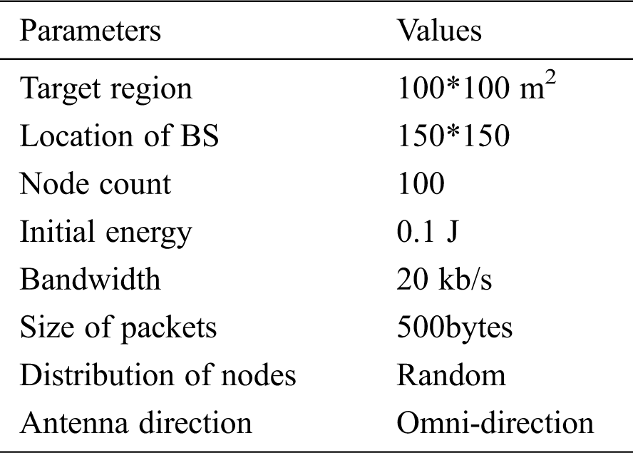
Fig. 4 demonstrates the energy efficiency analysis of the EAANFC-MR technique interms of energy consumption. The figure depicted that the TCBDGA model has been found to be ineffective by attaining maximum energy dissipation. Also, the FRLDG model has tried to show slightly better energy dissipation over the earlier method. Followed by, the MOBFO-EER model has depicted moderate results with the average energy dissipation over the earlier methods. Along with that, the FEEC-IIR and FF models have reached a near optimal energy dissipation under varying IoT node count. At last, the EAANFC-MR model has accomplished minimum energy dissipation over all the other compared methods. For instance, under the maximum node count of 500, the EAANFC-MR model has reached a lower energy dissipation of 114mJ whereas the FF, FEEC-IIR, MOBFO-EER, FRLDG, and TCBDGA models have obtained a higher energy consumption of 42mJ, 45mJ, 55mJ, 65mJ, and 135mJ respectively.
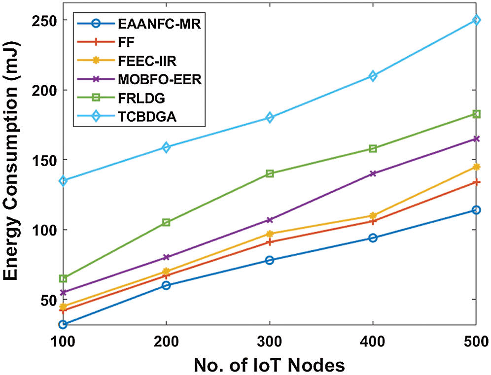
Figure 4: Analysis of EAANFC-MR model interms of energy consumption
Fig. 5 investigates the network lifetime analysis of the EAANFC-MR technique with a set of existing methods. The figure showcased that the minimum network lifetime is obtained by the TCBDGA algorithm. At the same time, the FRLDG model has reached a slightly higher network lifetime over the earlier model. But the MOGFO-EER model has tried to attain even better network lifetime. Likewise, the FEEC-IIR and FF models have achieved somewhat satisfactory network lifetime. However, the EEANFC-MR model has demonstrated superior results with the maximum network lifetime. For instance, under the node count of 500, the EAANFC-MR model has reached to a higher network lifetime of 5900 rounds whereas the FF, FEEC-IIR, MOBFO-EER, FRLDG and TCBDGA models have resulted to a minimum network lifetime of 5600, 5600, 5000, 4800 and 4300 rounds correspondingly.
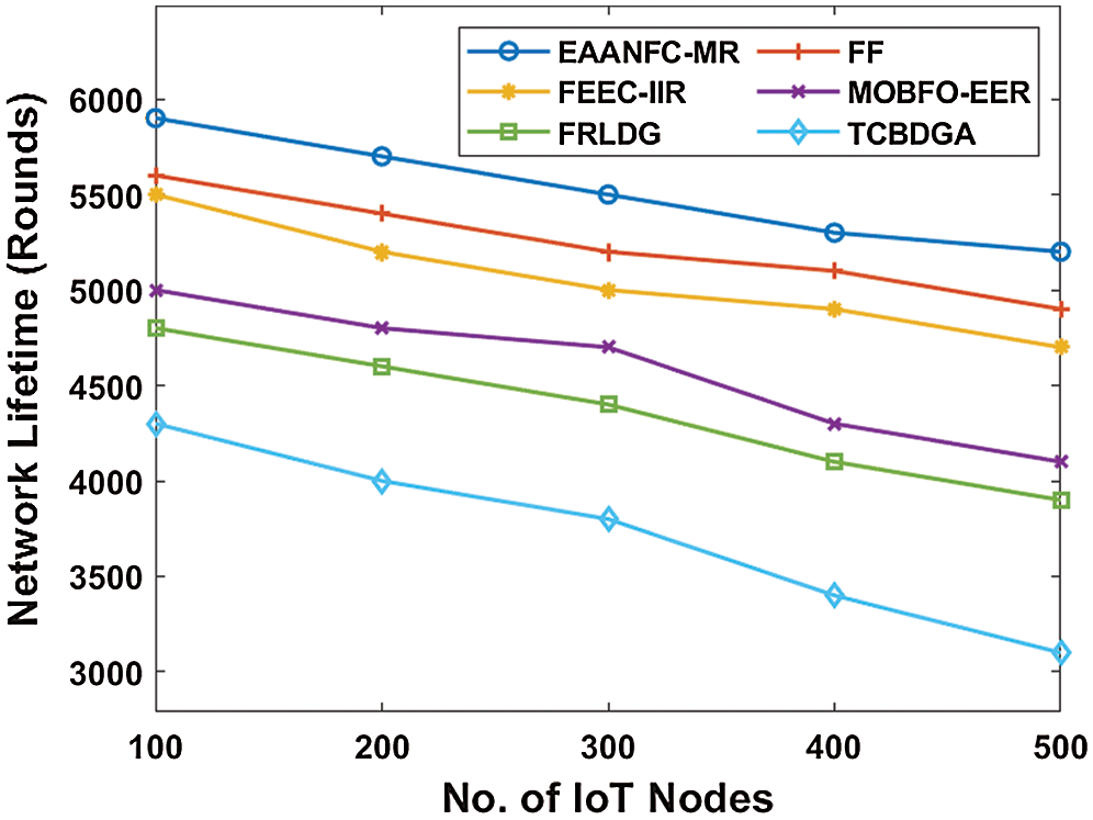
Figure 5: Analysis of EAANFC-MR model interms of Network lifetime
Fig. 6 examines the PDR analysis of the EAANFC-MR model with a collection of previous approaches. The figure portrayed that the low PDR is achieved by the TCBDGA scheme. Simultaneously, the FRLDG framework has accomplished moderate PDR than the previous models. However, MOGFO-EER technology has managed to achieve slightly better PDR. Similarly, the FEEC-IIR and FF methods have gained considerable PDR. But, the EEANFC-MR technique has depicted supreme outcomes with higher PDR. For sample, under the node value of 500, the EAANFC-MR framework has attained maximum PDR of 98% while the FF, FEEC-IIR, MOBFO-EER, FRLDG and TCBDGA methodologies have achieved least PDR of 96%, 95%, 94%, 92%, and 88% respectively.

Figure 6: Analysis of EAANFC-MR model interms of PDR
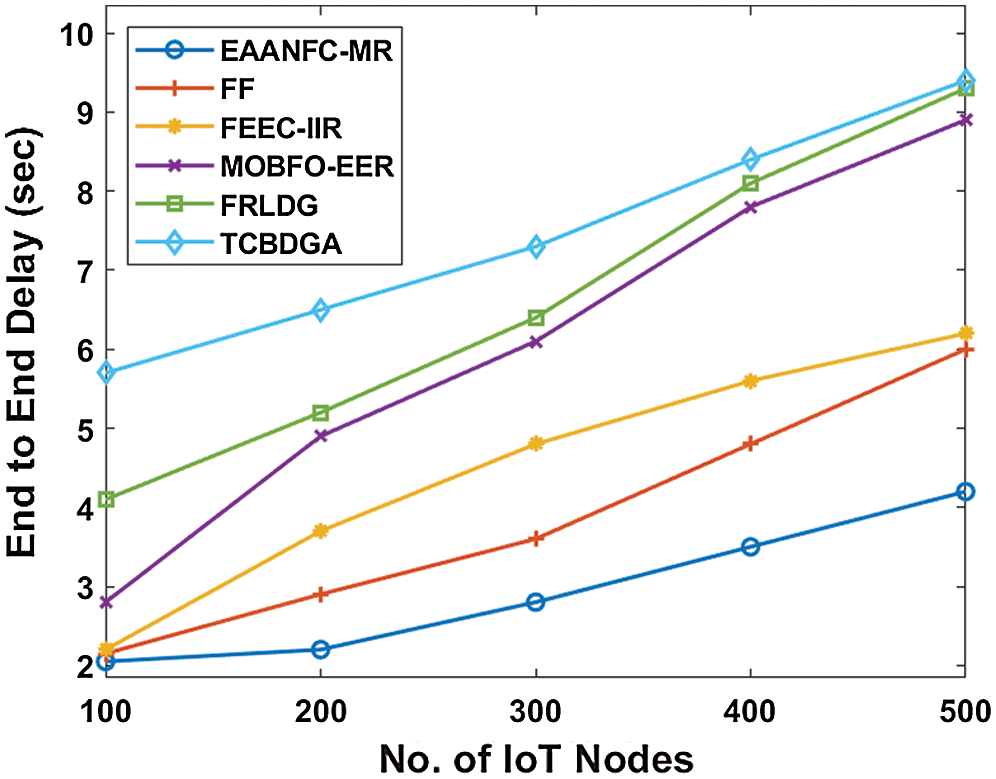
Figure 7: Analysis of EAANFC-MR model interms of ETE delay
Fig. 7 showcases the ETE delay analysis of the EAANFC-MR method with a group of earlier approaches. The figure implied that the TCBDGA approach has meant to be insignificant by reaching a higher ETE delay. Moreover, the FRLDG framework has attempted to display a moderate ETE delay when compared with the traditional framework. Besides, the MOBFO-EER technique has showcased better outcomes with the average ETE delay than the classical models. In line with this, the FEEC-IIR and FF methodologies have gained closer and identical ETE delay under various IoT node count. Simultaneously, the EAANFC-MR approach has achieved a low ETE delay than the traditional approaches. For sample, under the higher node count of 500, the EAANFC-MR scheme has obtained a minimum ETE delay of 4.2s while the FF, FEEC-IIR, MOBFO-EER, FRLDG, and TCBDGA frameworks have attained maximum ETE delay of 6s, 6.2s, 8.9s, 9.3s, and 9.4s correspondingly.
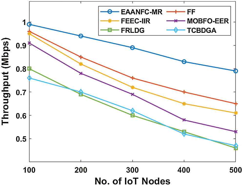
Figure 8: Analysis of EAANFC-MR model interms of Throughput
Fig. 8 analyzes the throughput analysis of the EAANFC-MR model with a set of previous approaches. The figure implied that the lower throughput is gained by the TCBDGA model. Meantime, the FRLDG framework has achieved considerable throughput over the compared method. However, MOGFO-EER technology has managed to reach slightly better throughput. Similarly, the FEEC-IIR and FF methods have accomplished better throughput. Therefore, the EEANFC-MR approach has illustrated qualified results with higher throughput. For illustration, under the node count of 500, the EAANFC-MR framework has achieved maximum throughput of 0.79Mbps and the FF, FEEC-IIR, MOBFO-EER, FRLDG, and TCBDGA technologies have accomplished low throughput of 0.65, 0.61, 0.53, 0.46, and 0.47 Mbps respectively.
Fig. 9 illustrated the packet loss ratio analysis of the EAANFC-MR with a collection of classical approaches. The figure illustrated that the TCBDGA framework is referred to as worse by achieving a higher packet loss ratio. Moreover, the FRLDG technique has managed to demonstrate a considerable packet loss ratio over the compared model. Then, the MOBFO-EER scheme has showcased better results with the average packet loss ratio when compared with previous technologies. Along with that, the FEEC-IIR and FF approaches have attained closer optimal packet loss ratio under distinct IoT node count.
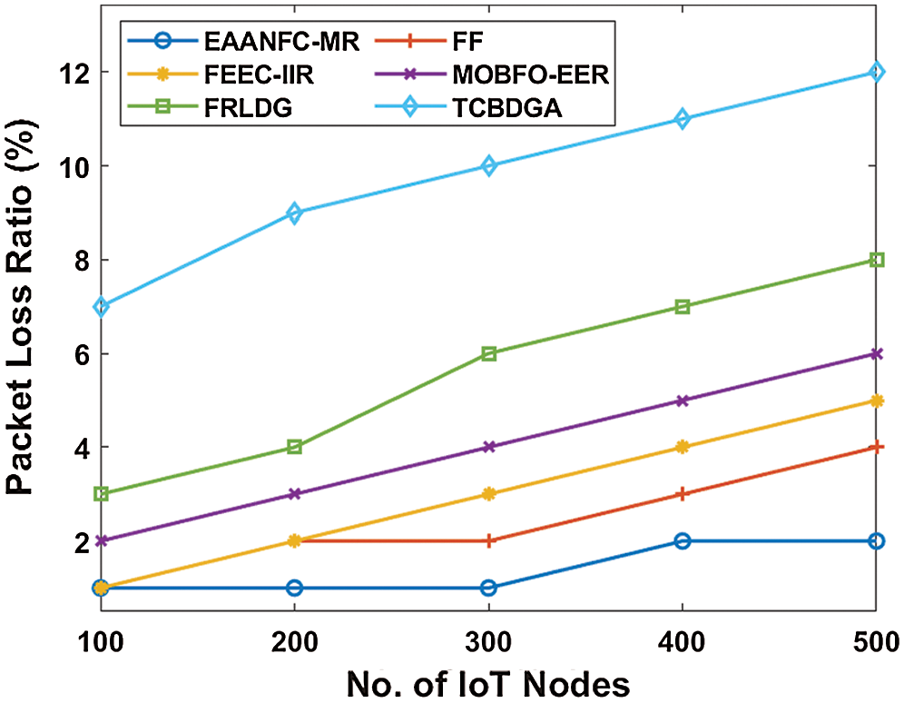
Figure 9: Analysis of EAANFC-MR model interms of the packet loss ratio
Consequently, the EAANFC-MR model has gained the least packet loss ratio over all the previous approaches. For example, under the higher node count of 500, the EAANFC-MR approach has achieved a minimal packet loss ratio of 2% whereas the FF, FEEC-IIR, MOBFO-EER, FRLDG, and TCBDGA models have accomplished maximum packet loss ratio of 4%, 5%, 6%, 8%, and 12% respectively.
Since IoT devices exist in WSN with built-in batteries, power efficiency is a problem that must be overcome. This paper has established a new routing protocol based on the IoT-assisted WSN cluster called the EAANFC-MR technique. The proposed EAANFC-MR is operated in two main phases: EAANFC-based and multihop. In order to determine the best set of CHs, the EAANFC technique with 3 input parameters is implemented. The MR technique is then implemented by QOBFO to detect the shortest path to contact between clusters. Finally, the method of data transfer will be performed. A comprehensive comparative analytical finding have ensured superior energy dissipation, lifespan, PDR, packet loss, transmission and delay efficiency in EAANFC-MR model. Using data aggregation techniques to improve the efficiency of the EAANFC MR model in the future.
Funding Statement: The authors received no specific funding for this study.
Conflicts of Interest: The authors declare that they have no conflicts of interest to report regarding the present study.
1. A. Forster, “Introduction to wireless sensor networks,” 1stEdition, Hoboken, New Jersey, USA: John Wiley and Sons, pp.1–226,2016. [Google Scholar]
2. J. Yick, B. Mukherjee and D. Ghosal, “Wireless sensor network survey,” Computer Networks, vol. 52, no. 12, pp. 2292–2330, 2008. [Google Scholar]
3. F. Bajaber and I. Awan, “An efficient cluster-based communication protocol for wireless sensor networks,” Telecommunication Systems, vol. 55, no. 3, pp. 387–401, 2014. [Google Scholar]
4. J. Lee and W. Cheng, “Fuzzy-logic-based clustering approach for wireless sensor networks using energy predication,” IEEE Sensors Journal, vol. 12, no. 9, pp. 2891–2897, 2012. [Google Scholar]
5. R. Mhemed, N. Aslam, W. Phillips and F. Comeau, “An energy efficient fuzzy logic cluster formation protocol in wireless sensor networks,” Procedia Computer Science, vol. 10, pp. 255–262, 2012. [Google Scholar]
6. D. Izadi, J. Abawajy and S. Ghanavati, “An alternative clustering scheme in WSN,” IEEE Sensors Journal, vol. 15, no. 7, pp. 4148–4155, 2015. [Google Scholar]
7. N. A. Pantazis, S. A. Nikolidakis and D. D. Vergados, “Energy-efficient routing protocols in wireless sensor networks: A survey,” IEEE Communications Surveys & Tutorials, vol. 15, no. 2, pp. 551–591, 2013. [Google Scholar]
8. A. A. A. Ari, B. O. Yenke, N. Labraoui, I. Damakoa and A. Gueroui, “A power efficient cluster-based routing algorithm for wireless sensor networks: honey bees swarm intelligence based approach,” Journal of Network and Computer Applications, vol. 69, no. 1, pp. 77–97, 2016. [Google Scholar]
9. A. Betzler, C. Gomez, I. Demirkol and J. Paradells, “CoAP congestion control for the internet of things,” IEEE Communications Magazine, vol. 54, no. 7, pp. 154–160, 2016. [Google Scholar]
10. R. Logambigai and A. Kannan, “Fuzzy logic based unequal clustering for wireless sensor networks,” Wireless Networks, vol. 22, no. 3, pp. 945–957, 2016. [Google Scholar]
11. P. G. V. Naranjo, M. Shojafar, H. Mostafaei, Z. Pooranian and E. Baccarelli, “P-SEP: A prolong stable election routing algorithm for energy-limited heterogeneous fog-supported wireless sensor networks,” Journal of Supercomputing, vol. 73, no. 2, pp. 733–755, 2017. [Google Scholar]
12. M. Elappila, S. Chinara and D. R. Parhi, “Survivable path routing in WSN for IoT applications,” Pervasive and Mobile Computing, vol. 43, no. 15, pp. 49–63, 2018. [Google Scholar]
13. G. Han, L. Zhou, H. Wang, W. Zhang and S. Chan, “A source location protection protocol based on dynamic routing in WSNs for the social internet of things,” Future Generation Computer Systems, vol. 82, no. 2, pp. 689–697, 2018. [Google Scholar]
14. M. Fouladlou and A. Khademzadeh, “An energy efficient clustering algorithm for Wireless Sensor devices in Internet of Things,” in proc. 2017 Artificial Intelligence and Robotics (IRANOPENQazvin, Vol.5, pp. 39–44, 2017. [Google Scholar]
15. J. Shen, A. Wang, C. Wang, P. C. K. Hung and C. Lai, “An efficient centroid-based routing protocol for energy management in WSN-assisted IoT,” IEEE Access, vol. 5, pp. 18469–18479, 2017. [Google Scholar]
16. J. H. Park and N. Y. Yen, “Advanced algorithms and applications based on IoT for the smart devices,” Journal of Ambient Intelligence and Humanized Computing, vol. 9, no. 4, pp. 1085–1087, 2018. [Google Scholar]
17. A. A. Kamil, M. K. Naji and H. A. Turki, “Design and implementation of grid based clustering in WSN using dynamic sink node,” Bulletin of Electrical Engineering and Informatics, vol. 9, no. 5, pp. 2055–2064, 2020. [Google Scholar]
18. A. Kaur, P. Gupta and R. Garg, “Soft computing techniques for clustering in WSN,” IOP Conf. Series: Materials Science and Engineering, vol. 1022, no. 1, pp. 1–11, 2020. [Google Scholar]
19. D. Kalaimani, Z. Zah and S. Vashist, “Energy-efficient density-based fuzzy c-means clustering in WSN for smart grids,” Australian Journal of Multi-Disciplinary Engineering, vol. 4, no. 5, pp. 1–16, 2020. [Google Scholar]
20. Lekhraj, A. Singh, A. Kumar and A. Kumar, “Multi parameter based load balanced clustering in WSN using MADM technique,” in proc. 4th Int. Conf. on Electronics, Communication and Aerospace Technology (ICECACoimbatore, India, pp. 814–820, 2020. [Google Scholar]
21. P. K. Kashyap, S. Kumar, U. Dohare, V. Kumar and R. Kharel, “Green computing in sensors-enabled internet of things: Neuro fuzzy logic-based load balancing,” Electronics, vol. 8, no. 4, pp. 1–22, 2019. [Google Scholar]
22. H. Chen, L. Wang, J. Diand and S. Ping, “Bacterial foraging optimization based on self-adaptive chemotaxis strategy,” Computational Intelligence and Neuroscience, vol. 2020, no. 2630104, pp. 1–15, 2020. [Google Scholar]
23. D. Guha, P. Royand and S. Banerjee, “Quasi-oppositional backtracking search algorithm to solve load frequency control problem of interconnected power system,” Iranian Journal of Science and Technology, Transactions of Electrical Engineering, vol. 44, no. 2, pp. 781–804, 2020. [Google Scholar]
24. P. K. Roy and S. Bhui, “Multi objective quasi-oppositional teaching learning based optimization for economic emission load dispatch problem,” International Journal of Electrical Power & Energy Systems, vol. 53, no. 3, pp. 937–948, 2013. [Google Scholar]
 | This work is licensed under a Creative Commons Attribution 4.0 International License, which permits unrestricted use, distribution, and reproduction in any medium, provided the original work is properly cited. |