DOI:10.32604/iasc.2021.017703
| Intelligent Automation & Soft Computing DOI:10.32604/iasc.2021.017703 | |
| Article |
Novel Power Transformer Fault Diagnosis Using Optimized Machine Learning Methods
1Electrical Engineering Department, College of Engineering, Taif University, Taif, 21944, Saudi Arabia
2Department of Electrical Power and Machines Engineering, Faculty of Engineering, Tanta University, Tanta, 31511, Egypt
*Corresponding Author: Diaa-Eldin A. Mansour. Email: mansour@f-eng.tanta.edu.eg
Received: 05 February 2021; Accepted: 08 March 2021
Abstract: Power transformer is one of the more important components of electrical power systems. The early detection of transformer faults increases the power system reliability. Dissolved gas analysis (DGA) is one of the most favorite approaches used for power transformer fault prediction due to its easiness and applicability for online diagnosis. However, the imbalanced, insufficient and overlap of DGA dataset impose a challenge towards powerful and accurate diagnosis. In this work, a novel fault diagnosis for power transformers is introduced based on DGA by using data transformation and six optimized machine learning (OML) methods. Four data transformation techniques are used with the dissolved gasses of transformer oils to reduce the high overlap of dataset samples. The OML methods used for transformer fault diagnosis are decision tree, discriminant analysis, Naïve Bayes, support vector machines, K-nearest neighboring, and ensemble classification methods. The six OML methods are implemented by MATLAB/Software based on 542 dataset samples collected from laboratories and literature. In this regard, 361 dataset samples were used for training, while 181 dataset samples were used for testing. The transformer fault diagnosis based on the OML methods had superior predicting accuracy compared to conventional and artificial intelligence methods.
Keywords: Transformer fault diagnosis; dissolved gas analysis; machine learning; data transformation
Nomenclature
| H2: | Hydrogen |
| CO: | Carbon monoxide |
| CH4: | Methane |
| CO2: | Carbon dioxide |
| C2H6: | Ethane |
| C2H2: | Acetylen |
| C2H4: | Ethylene |
| DGA: | Dissolved gas analysis |
| PD: | Partial discharge |
| DT: | Decision tree |
| T1: | Low thermal faults |
| DA: | Discriminant analysis |
| T2: | Medium thermal faults |
| NB: | Naïve Bayes |
| T3: | High thermal faults |
| SVM: | Support vector machine |
| D1: | Low energy discharges |
| KNN: | K-nearest neighboring |
| D2: | High energy discharges |
| EN: | Ensemble method |
| OML: | Optimized machine learning |
| BO: | Bayesian optimization |
| | The ith percentage gas ratios |
| | Relative erro |
| | The ith gas concentration in ppm |
| | The number of predicted sample |
| TDCG: | The summation of all gas concentrations |
| | The total number of training samples |
| AI: | Artificial intelligent |
| Mod-Rog: | Rogers’ modified four-ratio |
| NPR: | Neural pattern recognition |
| Mod-IEC: | Modified IEC 60599 code |
The power transformer is one of the most important equipment in electrical power systems. Accordingly, the early detection of transform faults is very important to enhance power system reliability [1]. The power transformers are subjected to electrical and thermal stresses, which can cause decomposition in the insulation oil with a subsequent generation of dissolved gasses. The more common gasses in transformer oil are Hydrogen (H2), Methane (CH4), Ethane (C2H6), Ethylene (C2H4), Acetylene (C2H2), carbon monoxide (CO), carbon dioxide (CO2) [2,3]. In most researches, the first five dissolved combustible gasses (H2, CH4, C2H6, C2H4, and C2H2) are used for predicting the power transformer fault types, since CO and CO2 are only used for predicting the insulating papers degradation state [4,5]. The different transformer fault types produced due to electric and thermal stresses are classified as partial discharge (PD), low and high energy discharges (D1 and D2), and low, medium, and high thermal faults (T1, T2, and T3) [6].
Power transformer fault type prediction based on dissolved gas analysis (DGA) was carried out by some conventional methods, artificial intelligence based methods, and machine learning based methods. The conventional methods are divided into ratio methods and graphical methods. The ratio methods include Doernenburg ratio, Rogers’ three and four-ratio, and IEC 60599 code methods [7,8]. The graphical methods include the Duval triangle [9], Duval and Mansour pentagon [10,11], and Gouda heptagon [12] methods. The conventional methods are simple to implement, but they have poor detecting accuracy for power transformer fault types. The artificial intelligence based methods used for transformer fault diagnosis include various methods such as: neural networks [3,13,14], fuzzy logic [15–17], Neuro-fuzzy [18], particle swarm-fuzzy logic [19,20], support vector machines [21–23], hybrid grey wolf optimization technique [4]. The artificial intelligence based methods has high predicting accuracy for transformer fault diagnosis compared to the conventional ratio and graphical methods, but they necessitate large dataset for implementation. Moreover, more accurate methods are needed to assure the highest reliability level of electrical grids. As a result, machine learning based methods were proposed as superior methods for power transformer diagnostics based on DGA [24]. However, the selection of governing parameters in machine learning based methods is crucial for effective application of these methods.
From this viewpoint, it is proposed in this work to develop a novel power transformer fault diagnosis based on six optimized machine learning (OML) classification methods. The six OML classification methods are decision tree (DT), discriminant analysis (DA), Naïve Bayes (NB), support vector machines (SVM), K-nearest neighboring (KNN), and ensemble methods (EN). These are applied to 542 dataset samples collected from laboratories and literature. The collected samples have a high overlap degree among different fault types. To enhance the OML predicting accuracy, four data transformation techniques are implemented. The four data transformations are logarithmic, normalization, standardization, and percentage gas ratio techniques. The predicting accuracy is compared among different OML classification methods and data transformation techniques. The different methods are implemented using MATLAB/software classification toolbox.
The organization of the next sections is as follows. Section two introduces data transformation techniques and methodology, while section three presents the results of OML methods with different data transformation techniques. Section four introduces the validation of the proposed method and comparisons with conventional and artificial intelligence based methods. Finally, section five presents conclusions and recommendations.
2 Data Transformation Techniques and Solution Methodology
2.1 Data Transformation Techniques
The proposed OML methods are carried out and implemented based on 542 dataset samples. The dataset samples are collected from literature, utilities, Egyptian Electricity Holding Company (EEHC) in Egypt, and Technology Information Forecasting and Assessment Council (TIFAC) in India [6,9,21,25–28]. This variety of dataset samples are used in this work to assure the reliability of the proposed fault diagnosis. The dataset distribution is divided into two datasets. The first dataset is used for the training process (361 samples, 66.67% from overall dataset samples), while the second is used for the testing process (181 samples, 33.33% from overall dataset samples). The distribution of the training and testing datasets is introduced in Tab. 1 against transformer fault types.
Table 1: Distribution of training and testing dataset samples against fault types
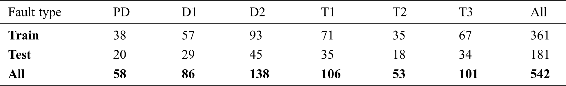
Fig. 1 introduces the distribution of H2, CH4, C2H6, and C2H2 versus the different transformer fault types. The distribution of the different gasses against different fault types has a high degree of overlap, which requires a transformation technique of the dataset before applying the OML methods to enhance their predicting accuracy.
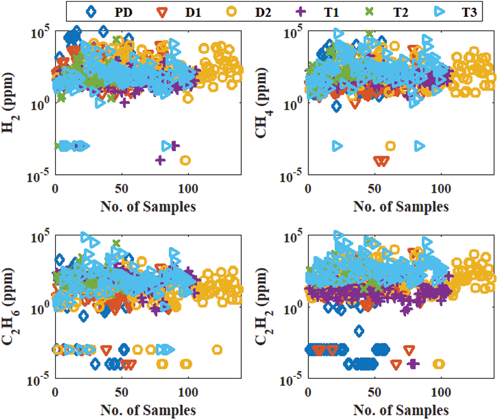
Figure 1: Distribution of H2, CH4, C2H6, and C2H2 versus the different transformer fault types
2.1.1 Gas percentage transformation
In the gas percentage transformation, the input gas ratio to the OML methods can be expressed as follows:
where,
2.1.2 Logarithmic transformation
In the logarithmic transformation, the input gas ratio to the OML methods can be presented as follows:
2.1.3 Normalization transformation
In the normalization transformation, the input gas ratio to the OML methods can be calculated as follows:
2.1.4 Standardization transformation
In the standardization transformation, the input gas ratio to the OML methods can be estimated as follows:
where,
Fig. 2 introduces the distribution of H2, CH4, C2H6, and C2H2 against the different transformer fault types with different transformation techniques. It is illustrated that the overlap of gas distribution with different faults after applying transformation techniques is lower than that of raw gas concentrations in Fig. 1, especially with gas percentage transformation technique.
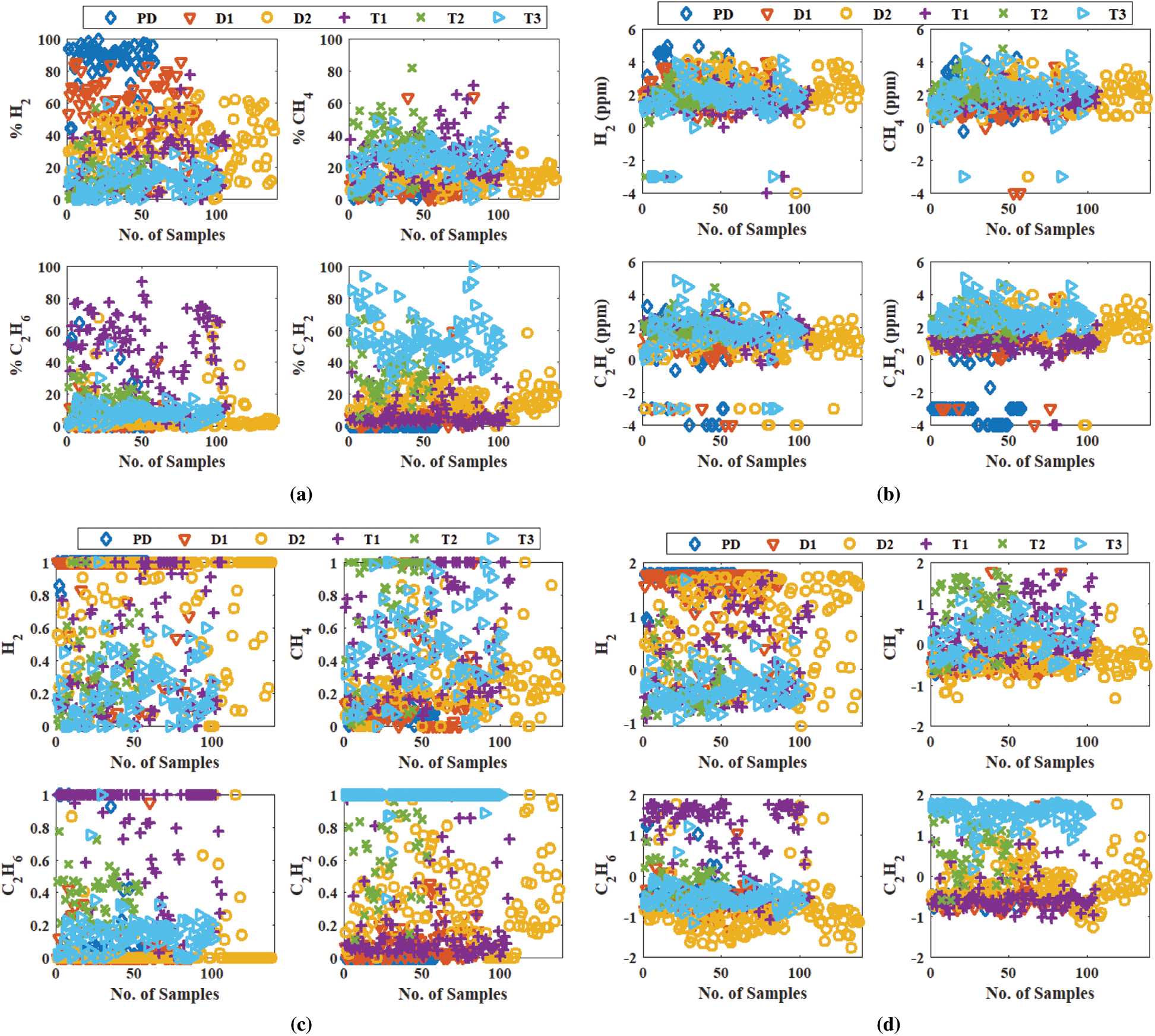
Figure 2: Distribution of H2, CH4, C2H6, and C2H2 versus the different transformer fault types with different transformation techniques. (a) Gas percentage (b) Logarithmic (c) Normalization (d) Standardization
2.2 Solution Methodology and OML Methods
The OML methods are optimized during the training process by Bayesian optimization (BO). The BO technique is one of the most effective approaches that was used with OML methods to identify their hyperparameters [29]. The BO is used to determine the optimized parameters of each method to enhance its predicting accuracy. For example, the optimal parameters of the KNN method are number of neighbors, distance metric, distance, weight, standardize data, while that of the EN method is ensemble method, the maximum number of splits, number of learners, and learning rate. The BO is used to determine the optimal parameters based on period calculation, and then the probabilistic model is used to evaluate the optimal parameters by applying the different probability values to select the suitable one that gives the highest probability [30]. The BO model used for determining the optimal parameters of OML methods was expressed in [30,31]. The optimization models of the six OML methods are carried out by MATLAB/software 2020b classification learner toolbox [32]. The optimized model of each method with different transformation data are then used for predicting new dataset samples denoted as testing samples.
The procedure of selection methodology is summarized in the following steps:
1. Divide dataset samples into two sets: the first set (361 samples) is used for the training process, while the second one is used for testing purposes (181 samples).
2. Choose the validation technique: the cross-validation folds with 10 folds is chosen for the training process.
3. Choose classifier options: the optimization technique (BO), acquisition options (expected improvement by per second plus) and the total number of iterations of 30.
4. Choose the OML classifier method.
5. Start the training process: the model hyperparameters are determined using BO and the predicting accuracy of the training dataset is obtained.
6. Access classifier method parameters and performance.
7. Export the classifier model of the selected OML method.
8. Repeat steps 3 up to 7 with the different OML methods.
9. Use the optimized models of the OML methods to predict the transformer fault types for the testing dataset samples.
10. Compere between the predicting accuracy of the OML methods to determine the best one.
In this work, MATLAB/software 2020b classification learner toolbox is used as a platform for the optimization classifiers. It is consists of six OML methods. The six OML methods are DT, DA, NB, SVM, KNN, and EN. A brief summary of the six OML methods used in this study for classification learner toolbox is introduced as follows:
• Decision tree (DT)
The decision tree consists of the root node, branches, internal nodes, and leaf nodes [33]. The classification process of the DT method is carried out by evaluating the information of each attribute and using them to split the datasets into different subsets flowing from the root node through branching and internal nodes until attain the final decision class at the leaf nodes [34]. The BO technique is used to determine the optimal hyperparameters of the DT, which are a maximum number of splits and split criterion. This process is repeated by removing the branches that aren't helpful in the classification process until the final decision tree model is obtained.
• K-nearest neighbor (KNN)
The KNN method is an effective OML method that is used in different classification applications [34]. The main idea of the KNN method is to determine the training dataset samples for each class that have the closest distance to a given query position [35]. The BO is used to determine the optimal hyperparameters of the KNN method to obtain the highest classification accuracy. The KNN optimization hyperparameters are number of neighbors, distance metric, distance weight, and standardize data.
• Support vector machines (SVM)
The SVM classifies data by building a number of hyperplanes that separate between the classes on the training dataset [21]. SVM is categorized as a kernel method. The hyperline is chosen to a wide separation between the classes. The kernel function is used to determine the path of the hyperline. SVM has the advantages of good predicting classification accuracy, but it required a long time for the training process. The BO is used to estimate the optimal parameters of the SVM model during the training process. The optimal parameters of the SVM method are kernel function, kernel scale, box constraint level, meticulous method, and standardize data.
• Ensemble method (EN)
The EN method is similar to the DT method, so that it consists of the root node, branches, internal nodes, and leaf nodes. The EN method is generating a subset sample from the main dataset samples and using the main dataset and the generated dataset for the training process [36]. It required a long time for the training process compared to the DT and KNN methods [34]. The BO is used to estimate the optimal parameters of the EN model during the training process. The optimal parameters of the EN method are the ensemble method, maximum number of splits, number of learners, and learning rate.
• Naïve Bayes (NB)
The NB is one of the classifiers that depends on the Bayes theorem on the classification process [37]. In this method, the classification process assumes that the input features are independent to determine the output classes. The NB is faster than SVM and EN for the training process, and it is suitable for training large dataset samples. The optimal parameters of the NB are determined by BO during the training stage. The optimal parameters of the NB method are distribution names and kernel type.
• Discriminant analysis (DA)
The DA is one of the classifiers that depends on the Bayes theorem on the classification process [38]. The DA analysis types are linear and quadratic discriminant types. The DA is faster than SVM and EN for the training process, but it has a low predicting accuracy of the classification process. The optimal parameters of the DA are determined by BO during the training stage. The optimization parameter of the DA method is discriminant type.
The six OML classification methods were implemented using a classification learner toolbox of MATLAB/software 2020b. The 542 dataset samples were used for both training (361 samples) and testing (181 samples) stages of six OML methods. The training process of six OML methods based on the raw dataset and the four data transformation techniques was introduced in this section.
The relative error of the six OML methods during the training stage can be evaluated as follows:
where
Fig. 3 illustrates the relative minimum error during the training stage of the six OML methods with raw dataset training samples (361 samples). The raw dataset consists of 361 samples with five gasses (H2, CH4, C2H6, C2H4, and C2H2). The results illustrate that the minimum relative error of the six OML methods decreased with training iteration number and reached their minimum values after several iterations. The KNN and EN have a minimum relative error at the end of a training stage that close to 0.23, which is a relatively large value. So that, the predicting accuracy of the six OML methods is relatively low for both training and testing stages, as introduced in Tab. 2. The results illustrate the low predicting accuracy for all methods during training and testing stages, especially the DA and NB methods. Also, the results illustrate that the EN method has the highest predicting accuracy with 78.39% and 84.53% for training and testing stages, respectively.
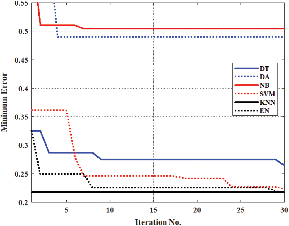
Figure 3: Minimum error of the six OML methods during the training stage with the raw input dataset.
Table 2: Predicting accuracy for both the training and testing stages with the raw input dataset
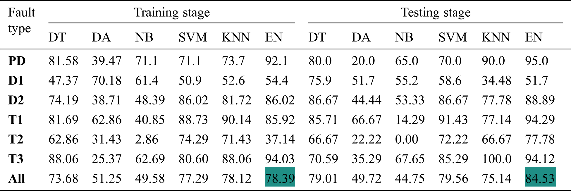
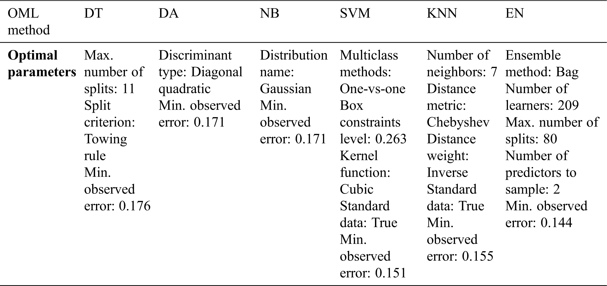
Fig. 4 presents the minimum error against iteration number during the training process with the six OML methods using the four suggested data transformation techniques (logarithmic, normalization, standardization, and gas percentage ratios). The results illustrate that the minimum errors with the six OML methods during the training stages with gas percentage transformation techniques are smaller than that of normalization, standardization, and logarithmic transformation techniques. The optimal parameters of the six OML methods with gas percentage transformation are introduced in Tab. 3.
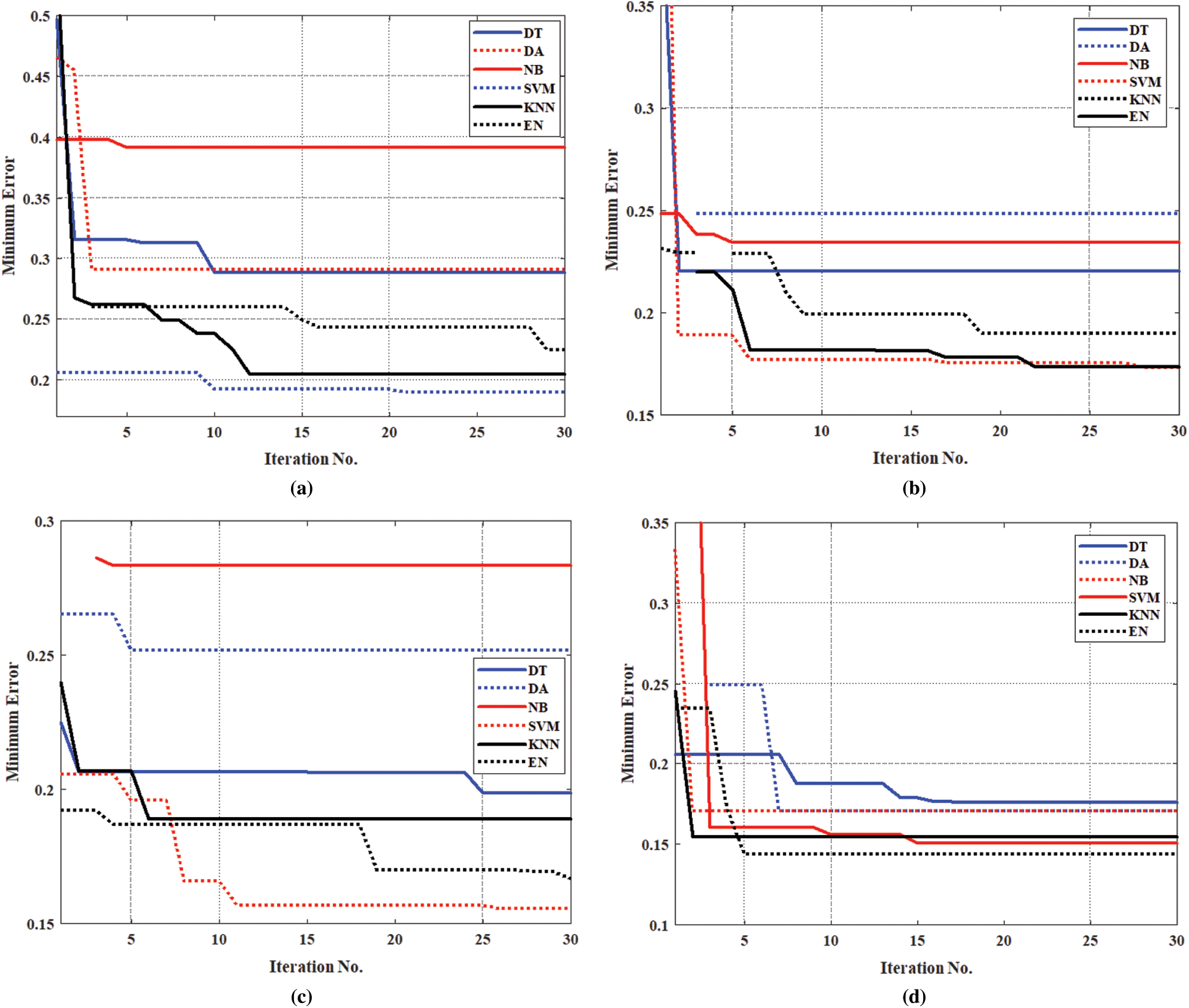
Figure 4: The minimum error versus iteration number during the training process with the six OML methods and four data transformation techniques. (a) Logarithmic transformation (b) Standarization transformation (c) Normalization transformation (d) Gas percentage transformation
Fig. 5 presents the predicting accuracy for both training and testing dataset samples of the six suggested OML methods with the four data transformation techniques. The results illustrate that the predicting accuracy with gas percentage transformation is better than other transformation techniques. The predicting accuracy of testing data sets (181 samples) are 83.43%, 83.83%, 85.08%, 85.08%, 89.50%, and 90.61% for DA, NB, DT, KNN, SVM, and EN methods, respectively. The highest predicting accuracy with testing dataset samples is obtained by the EN method with 90.61%.
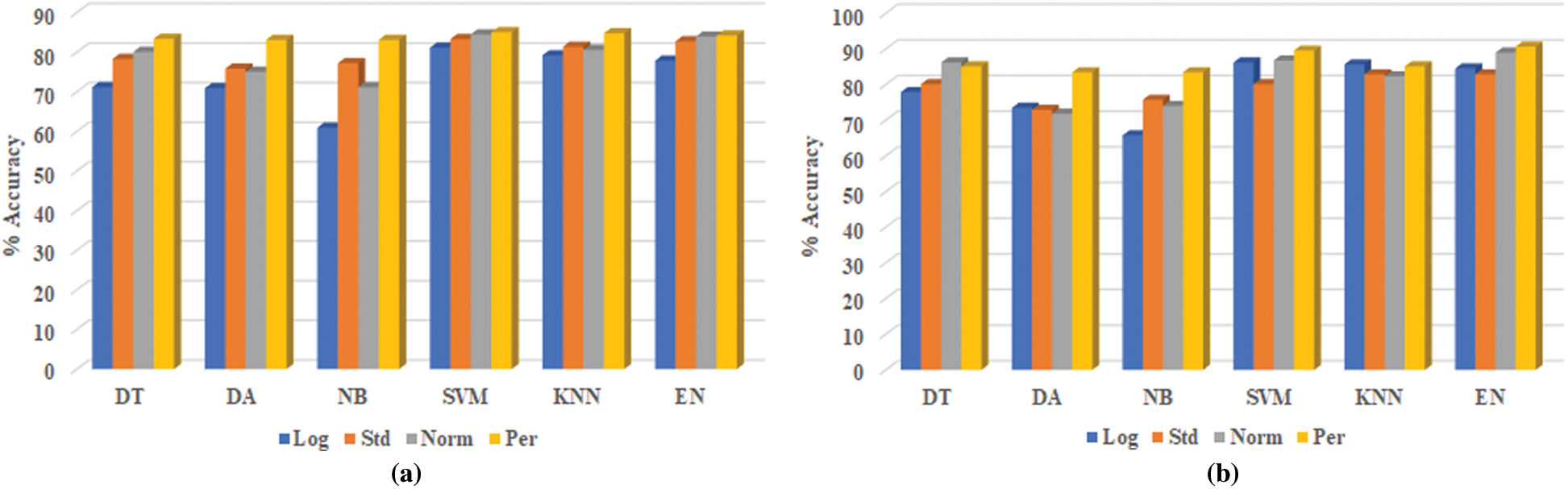
Figure 5: The predicting accuracy of the six OML methods with the four data transformation techniques for training and testing stages. a) Training accuracy b) Testing accuracy
Table 3: The optimal parameters of six OML methods with gas percentage transformation
4.1 Comparison between the Proposed Model and Other Methods
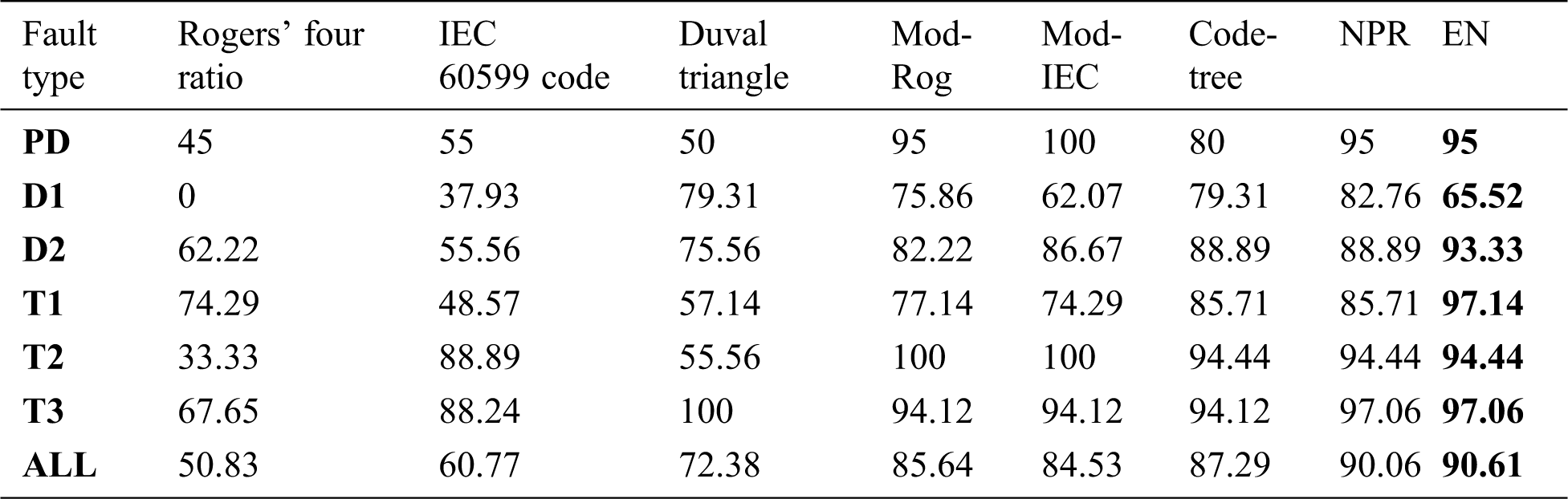
The predicting accuracy of the EN method is better than the other suggested OML methods so that it will be compared with other conventional and artificial intelligent (AI) methods that were recently published with the testing dataset samples (181 samples). The conventional methods used for comparisons are Rogers’ four-ratio, IEC 60599 code, and Duval triangle, while the AI methods are Rogers’ modified four-ratio [20], modified IEC 60599 code [20], the neural pattern recognition approach [3], and code-tree [4]. These comparisons are depicted in Tab. 4. The predicting accuracies are 50.83%, 60.77%, and 72.38% with Rogers’ four-ratio, IEC 60599 code, and Duval triangle methods, respectively, while that are 85.64%, 84.53%, 87.29%, 90.06%, and 90.61% for Rogers’ modified four-ratio (Mod-Rog), modified IEC 60599 code (Mod-IEC), code-tree, neural pattern recognition (NPR) approach, and the proposed EN method, respectively, with gas percentage transformation. The results indicate that the proposed EN method with the gas percentage transformation technique has the highest predicting accuracy.
Table 4: Comparison between the proposed EN method and conventional and AI methods with the testing dataset samples
4.2 Implementation of the Proposed Models in DGALab Software
The proposed models of OML classification methods (DT, DA, NB, SVM, KNN, and EN) with gas percentage transformation are implemented in DGALab software [39] to facilitate the transformer fault diagnosis for engineers in electrical utilities. They can insert the dissolved gasses directly into the software to obtain the corresponding fault types.
Fig. 6 presents a comparison between the proposed EN method with other methods on DGALab software using testing dataset samples (181 samples). It illustrates that the proposed EN method has good predicting accuracy that is better than other methods.
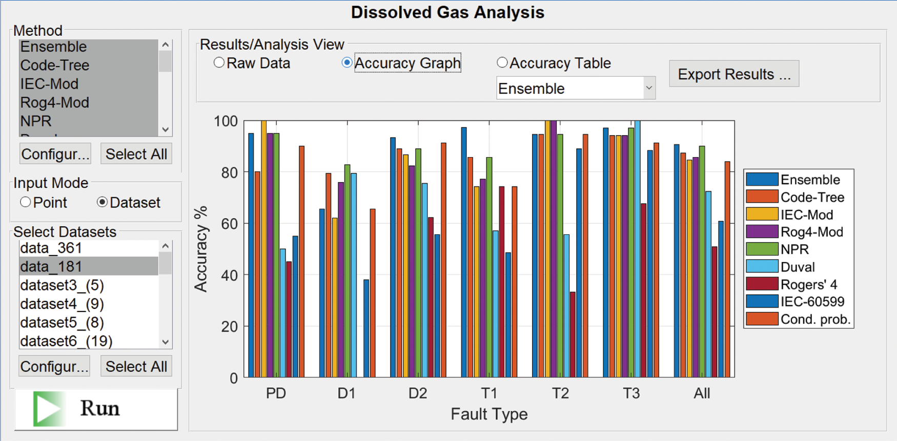
Figure 6: Comparison between the proposed EN method and the other methods on DGALab software using testing dataset samples
Fig. 7 shows the confusion matrix of the proposed EN method extracted from DGALab software with testing dataset samples (181 samples). The predicting accuracy for transformer fault types are 95%, 65.52%, 93.33%, 97.14%, 94.44%, 97.06%, and 90.61% in predicting PD, D1, D2, T1, T2, T3, and all samples, respectively.
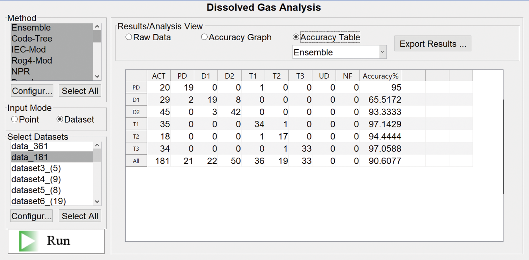
Figure 7: Confusion matrix of the proposed EN method extracted from DGALab software with testing dataset samples
In this paper, a novel power transformer fault type diagnosis has been developed using six OML classification methods with four data transformation techniques. The six OML methods used were DT, DA, NB, SVM, KNN, and EN methods. The four transformation techniques were implemented to enhance the fault predicting accuracy of the proposed methods. The data transformation techniques were logarithmic, normalization, standardization, and gas percentage transformations. The transformer fault detecting accuracy of the six OML methods with the gas percentage transformation was better than other transformation techniques, especially with SVM and EN methods. The predicting accuracy of the EN method with the testing dataset samples was 90.61%. The proposed model predicting accuracy was compared with conventional methods (Rogers’ four-ratio, IEC 60599 code, Duval triangle) and AI methods (Rogers’ modified four-ratio, modified IEC 60599 code, code-tree, and neural pattern recognition methods). The comparison validated the superiority of the proposed model. Furthermore, the six proposed OML methods were implemented in DGALab software to facilitate their implementation by electrical utilities for transformer fault diagnosis.
Funding Statement: The authors would like to acknowledge the financial support received from Taif University Researchers Supporting Project Number (TURSP-2020/61), Taif University, Taif, Saudi Arabia.
Conflicts of Interest: The authors declare that they have no conflicts of interest to report regarding the present study.
1. S. A. Wani, D. Gupta, M. U. Farooque and S. A. Khan, “Multiple incipient fault classification approach for enhancing the accuracy of dissolved gas analysis (DGA),” IET Science, Measurement & Technology, vol. 13, no. 7, pp. 959–967, 2019. [Google Scholar]
2. F. Jakob and J. J. Dukarm, “Thermodynamic estimation of transformer fault severity,” IEEE Trans. on Power Delivery, vol. 30, no. 4, pp. 1941–1948, 2015. [Google Scholar]
3. I. B. M. Taha, S. S. Dessouky and S. S. M. Ghoneim, “Transformer fault types and severity class prediction based on neural pattern-recognition techniques,” Electric Power Systems Research, vol. 191, no. 7, 9, pp. 106899, 2021. [Google Scholar]
4. A. Hoballah, D. A. Mansour and I. B. M. Taha, “Hybrid grey wolf optimizer for transformer fault diagnosis using dissolved gases considering uncertainty in measurements,” IEEE Access, vol. 8, pp. 139176–139187, 2020. [Google Scholar]
5. M. A. Izzularab, G. E. M. Aly and D. A. Mansour, “On-line diagnosis of incipient faults and cellulose degradation based on artificial intelligence methods,” in Proc. 2004 IEEE Int. Conf. on Solid Dielectrics, Toulouse, France, pp. 767–770, 2004. [Google Scholar]
6. M. Duval and A. dePablo, “Interpretation of gas-in-oil analysis using new IEC publication 60599 and IEC TC 10 databases,” IEEE Electrical Insulation Magazine, vol. 17, no. 2, pp. 31–41, 2001. [Google Scholar]
7. IEEE, IEEE Standard C57.104-2008-IEEE Guide for the Interpretation of Gases Generated in Mineral Oil-Immersed Transformers, 2009. [Google Scholar]
8. S. S. M. Ghoneim, I. B. M. Taha and N. I. Elkalashy, “Integrated ANN-based proactive fault diagnostic scheme for power transformers using dissolved gas analysis,” IEEE Transactions on Dielectrics and Electrical Insulation, vol. 23, no. 3, pp. 1838–1845, 2016. [Google Scholar]
9. M. Duval, “A review of faults detectable by gas-in-oil analysis in transformers,” IEEE Electrical Insulation Magazine, vol. 18, no. 3, pp. 8–17, 2002. [Google Scholar]
10. M. Duval and L. Lamarre, “Lamarre The Duval pentagon-a new complementary tool for the interpretation of dissolved gas analysis in transformers,” IEEE Electrical Insulation Magazine, vol. 30, no. 6, pp. 9–12, 2014. [Google Scholar]
11. D. A. Mansour, “A new graphical technique for the interpretation of dissolved gas analysis in power transformers,” in Proc. Annual Report Conf. on Electrical Insulation and Dielectric Phenomena, Montreal, QC, Canada, pp. 195–198, 2012. [Google Scholar]
12. O. E. Gouda, S. H. El-Hoshy and H. H. El-Tamaly, “Proposed heptagon graph for DGA interpretation of oil transformers,” IET Generation, Transmission & Distribution, vol. 12, no. 2, pp. 490–498, 2018. [Google Scholar]
13. V. Miranda and A. R. G. Castro, “Improving the IEC table for transformer failure diagnosis with knowledge extraction from neural networks,” IEEE Transactions on Power Delivery, vol. 20, no. 4, pp. 2509–2516, 2005. [Google Scholar]
14. S. Souahlia, K. Bacha and A. Chaari, “MLP neural network-based decision for power transformers fault diagnosis using an improved combination of Rogers and Doernenburg ratios DGA,” Int. Journal of Electrical Power & Energy Systems, vol. 43, no. 1, pp. 1346–1353, 2012. [Google Scholar]
15. I. B. M. Taha, S. S. M. Ghoneim and H. G. Zaini, “A fuzzy diagnostic system for incipient transformer faults based on DGA of the insulating transformer oils,” Int. Review of Electrical Engineering, vol. 11, no. 3, pp. 305–313, 2016. [Google Scholar]
16. Y.-C. Huang and H.-C. Sun, “Dissolved gas analysis of mineral oil for power transformer fault diagnosis using fuzzy logic,” IEEE Trans. on Dielectrics and Electrical Insulation, vol. 20, no. 3, pp. 974–981, 2013. [Google Scholar]
17. A. Abu-Siada, S. Hmood and S. Islam, “A new fuzzy logic approach for consistent interpretation of dissolved gas-in-oil analysis,” IEEE Trans. on Dielectrics and Electrical Insulation, vol. 20, no. 6, pp. 2343–2349, 2013. [Google Scholar]
18. T. Kari, W. Gao, D. Zhao, Z. Zhang and W. Mo, “An integrated method of ANFIS and Dempster-Shafer theory for fault diagnosis of power transformer,” IEEE Trans. on Dielectrics and Electrical Insulation, vol. 25, no. 1, pp. 360–371, 2018. [Google Scholar]
19. H. Zheng, Y. Zhang, J. Liu, H. Wei, J. Zhao et al., “A novel model based on wavelet LS-SVM integrated improved PSO algorithm for forecasting of dissolved gas contents in power transformers,” Electrical Power Systems Research, vol. 155, pp. 196–205, 2018. [Google Scholar]
20. I. B. M. Taha, A. Hoballah and S. S. M. Ghoneim, “Optimal ratio limits of rogers' four-ratios and IEC 60599 code methods using particle swarm optimization fuzzy-logic approach,” IEEE Trans. on Dielectrics and Electrical Insulation, vol. 27, no. 1, pp. 222–230, 2020. [Google Scholar]
21. K. Bacha, S. Souahlia and M. Gossa, “Power transformer fault diagnosis based on dissolved gas analysis by support vector machine,” Electrical Power Systems Research, vol. 83, no. 1, pp. 73–79, 2012. [Google Scholar]
22. J. Li, Q. Zhang, K. Wang, J. Wang, T. Zhou et al., “Optimal dissolved gas ratios selected by genetic algorithm for power transformer fault diagnosis based on support vector machine,” IEEE Trans. on Dielectrics and Electrical Insulation, vol. 23, no. 2, pp. 1198–1206, 2016. [Google Scholar]
23. Y. Zhang, X. Li, H. Zheng, H. Yao, J. Liu et al., “A fault diagnosis model of power transformers based on dissolved gas analysis features selection and improved krill herd algorithm optimized support vector machine,” IEEE Access, vol. 7, pp. 102803–102811, 2019. [Google Scholar]
24. M. E. Senoussaoui, M. Brahami and I. Fofana, “Combining and comparing various machine-learning algorithms to improve dissolved gas analysis interpretation,” IET Generation, Transmission & Distribution, vol. 12, no. 15, pp. 3673–3679, 2018. [Google Scholar]
25. S. Agrawal and A. K. Chandel, “Transformer incipient fault diagnosis based on probabilistic neural network,” in Proc. 2012 Students Conf. on Engineering and Systems, Allahabad, Uttar Pradesh, India, pp. 1–5, 2012. [Google Scholar]
26. J. Hu, L. Zhou and M. Song, “Transformer fault diagnosis method of gas chromatographic analysis using computer image analysis,” in Proc. 2012 Second Int. Conf. on Intelligent System Design and Engineering Application, Sanya, Hainan, China, pp. 1169–1172, 2012. [Google Scholar]
27. O. E. Gouda, S. H. El-Hoshy and H. H. El-Tamaly, “Proposed three ratios technique for the interpretation of mineral oil transformers based dissolved gas analysis,” IET Generation, Transmission & Distribution, vol. 12, no. 11, pp. 2650–2661, 2018. [Google Scholar]
28. E. Li, L. Wang and B. Song, “Fault diagnosis of power transformers with membership degree,” IEEE Access, vol. 7, pp. 28791–28798, 2019. [Google Scholar]
29. S. Putatunda and K. Rama, “A modifed Bayesian optimization based hyper-parameter tuning approach for extreme gradient boosting,” in Proc. 15th Int. Conf. on Information Processing (ICINPROBengaluru, India, pp. 1–6, 2019. [Google Scholar]
30. W. W. Tso, B. Burnak and E. N. Pistikopoulos, “HY-POP: Hyperparameter optimization of machine learning models through parametric programming,” Computers & Chemical Engineering, vol. 139, no. 1, pp. 106902, 2020. [Google Scholar]
31. J. Wu, X.-Y. Chen, H. Zhang, L.-D. Xiong, H. Lei et al., “Hyperparameter optimization for machine learning models based on Bayesian optimization,” Journal of Electronic Science and Technology, vol. 17, no. 4, pp. 100007, 2019. [Google Scholar]
32. Mathworks, “Classification learner app,” 2021. [Online] Available: https://ch.mathworks.com/help/stats/classification-learner-app.html. [Google Scholar]
33. D.Y. Yeh, C.H. Cheng and S.C. Hsiao, “Classification knowledge discovery in mold tooling test using decision tree algorithm,” Journal of Intelligent Manufacturing, vol. 22, no. 4, pp. 585–595, 2011. [Google Scholar]
34. A. Alqudsi and A. El-Hag, “Application of machine learning in transformer health index prediction,” Energies, vol. 12, no. 14, pp. 2694, 2019. [Google Scholar]
35. Y. Benmahamed, Y. Kemari, M. Teguar and A. Boubakeur, “Diagnosis of power transformer oil using KNN and Naïve Bayes classifiers,” in Proc. 2nd IEEE Int. Conf. on Dielectrics (ICDpp. 1–4, 2018. [Google Scholar]
36. P. K. Mishra, A. Yadav and M. Pazoki, “A novel fault classification scheme for series capacitor compensated transmission line based on bagged tree ensemble classifier,” IEEE Access, vol. 6, pp. 27373–27382, 2018. [Google Scholar]
37. L. Jiang, Z. Cai, H. Zhang and D. Wang, “Naive Bayes text classifiers: A locally weighted learning approach,” Journal of Experimental & Theoretical Artificial Intelligence, vol. 25, no. 2, pp. 273–286, 2013. [Google Scholar]
38. A. Tharwat, “Linear vs. quadratic discriminant analysis classifier: A tutorial,” Int Journal of Applied Pattern Recognition, vol. 3, no. 2, pp. 145–180, 2016. [Google Scholar]
39. S. I. Ibrahim, S. S. M. Ghoneim and I. B. M. Taha, “DGALab: An extensible software implementation for DGA,” IET Generation, Transmission & Distribution, vol. 12, no. 18, pp. 4117–4124, 2018. [Google Scholar]
 | This work is licensed under a Creative Commons Attribution 4.0 International License, which permits unrestricted use, distribution, and reproduction in any medium, provided the original work is properly cited. |