Intelligent Automation & Soft Computing DOI:10.32604/iasc.2021.017232
Article

Identification of Abnormal Patterns in AR (1) Process Using CS-SVM

Hongshuo Zhang1, Bo Zhu1,*, Kaimin Pang1, Chunmei Chen1 and Yuwei Wan2

1College of Mechanical and Electrical Engineering, Kunming University of Science & Technology, Kunming, 650500, China
2School of Engineering, Cardiff University, Cardiff, CF24 3AA, UK
*Corresponding Author: Bo Zhu. Email: zhubo20110720@163.com
Received: 24 January 2021; Accepted: 01 March 2021

Abstract: Using machine learning method to recognize abnormal patterns covers the shortage of traditional control charts for autocorrelation processes, which violate the applicable conditions of the control chart, i.e., the independent identically distributed (IID) assumption. In this study, we propose a recognition model based on support vector machine (SVM) for the AR (1) type of autocorrelation process. For achieving a higher recognition performance, the cuckoo search algorithm (CS) is used to optimize the two hyper-parameters of SVM, namely the penalty parameter c and the radial basis kernel parameter g . By using Monte Carlo simulation methods, the data sets containing samples of eight patters are generated in experiments for verifying the performance of the proposed model. The results of comparison experiments show that the average recognition rate of the proposed model reaches 96.25% as the autocorrelation coefficient is set equal to 0.5. That is apparently higher than those of the SVM model optimized by the particle swarm optimization (PSO) or the genetic algorithm (GA). Another experiment result demonstrates that the average recognition accuracy of the CS-SVM model also reaches higher than 95% for different autocorrelation levels. At last, a lot of data streams in or out of control are simulated to measure the ARL values. The results turn out that the model has an acceptable online performance. Therefore, we believe that the model can be used as a more effective approach for identification of abnormal patterns in autocorrelation process.

Keywords: Control chart pattern; support vector machine; cuckoo search algorithm; autocorrelation process; Monte Carlo simulation

1  Introduction

Nowadays, the integration concept of informatization and industrialization is gradually being proposed. Many new technologies emerge continuously, such as Virtual Manufacturing (VM), Computer Integrated Manufacturing (CIM), and Radio-frequency Identification (RFID), Concurrent Engineering (CE), [1–5]. Under such a background, manufacturing companies have begun to shift from incremental competition to stock competition. Subsequently, product quality has become one of the core competitiveness of enterprises for success. In the quality engineering field, statistical process control (SPC) is an essential means for ensuring quality in the manufacturing process, which takes the control chart as the basic tool. The use of traditional control charts must follow the premise that the observed data is independent identically distributed (IID). However, Shiau [6], Montgomery [7] pointed out that process data generally cannot approximately satisfy this premise in actual production process. When there are obvious autocorrelation phenomena presented in the observed data, the control chart often subjects to serious false alarm so that cannot detect true process abnormities effectively. Studies have shown that the autocorrelation phenomena significantly reduce the performance of control chart [8,9].

Academia has carried out much studies on process quality control with autocorrelation phenomena and proposed some approaches. The main category is to use statistical methods to eliminate the influence of autocorrelation on process data. The most representative one is the residual control chart. Montgomery and Woodall [10], Runger [11] proposed to use a fitted time series model to monitor the autocorrelation process. Because the controlled statistics’ residuals are independent identically distributed theoretically, the conventional Shewhart control chart can be used to monitor the residuals effectively. Sun [12] and Zhang [13] carried out much research on the residual control chart of the autocorrelation process and validated its effectiveness. With the development of artificial intelligence technology, pattern recognition methods based on machine learning are proposed and introduced into the process quality control field. There are also some machine learning based methods applied to the autocorrelation process that have been reported. For example, Cook and Chiu [14] used the BP neural network to recognize the autocorrelation process’ abnormal pattern. Experiments results show that it gets an advantage over the traditional statistical methods. Lin and Guh [15] applied a support vector machine (SVM) based model to abnormal pattern identification of autocorrelation process, which achieved better performance in both recognition accuracy and recognition speed. Zhu and Liu [16] proposed to use random forest for control chart pattern recognition in autocorrelation process, and verified that the performance of their model is better than that of the BP neural networks through simulation experiments.

SVM is a major machine learning method for classification, which has been also used frequently in control chart pattern recognition [17]. SVM first appeared in the 1990s. In contrast with the BP neural network’s pursuit of minimizing experience risk, SVM takes minimum of the structural risk as optimizing goal. In that, SVM can better deal with the over-fitting problem, and then often achieve better generalization performance, especially under small sample conditions. Simultaneously, it has much fewer parameters need to be adjusted and accommodate to high-dimensional features. The use of SVM involves selecting an appropriate kernel function and tuning of the related hyper-parameters, which is essential for its generalization performance. Currently, there are some algorithms, such as artificial fish swarm algorithm (AFSA), genetic algorithm (GA), artificial bee colony (ABC), grid search (GS) and particle swarm optimization (PSO) [18–22], have been applied in the optimization of the hyper-parameters of SVM. The cuckoo search algorithm (CS) is a type of combination optimization algorithm appeared in recent years. Compared with other algorithms, it has many advantages, for instance, simpler structure, easy to jump out of local optimal values, and fewer control parameters.

Due to the superiorities of the SVM and the CS, we proposed an autocorrelation process pattern recognition model based on SVM optimized by CS (CS-SVM), which is used as the pattern classifier. In this model, the hyper-parameters of the SVM are optimized by the CS to get higher generalization performance. To verify this model’s effectiveness, the data sets of basic patterns in AR (1) type of autocorrelation process, including normal pattern and seven types of abnormal pattern, are generated by Monte Carlo simulation method. Based on the data sets, some verification experiments are conducted. The experiment results show that the proposed model has apparent advantages over some other methods, both in recognition accuracy and training efficiency. At the same time, it has an acceptable on-line detecting performance.

The paper is structured as follows. In Section 2, some related theories and methods are reviewed. In Section 3, the model is established, and its structure graph is presented. In Section 4, the environment and data of the simulation experiments are given and results are discussed. Section 5 concludes the paper with a summary and remarks. Description of the Monte Carlo simulation functions of the eight patterns is displayed in the Appendix A.

2  Related Theories and Methods

2.1 AR (1) Autocorrelation Process

In the modern manufacturing process, the production tempo is getting faster and faster, and the automatic data acquisition technology is used more and more widely. As a result, the observed values of a specific variable get at different moment frequently present certain type of dependence with each other. That is called the autocorrelation phenomenon [23]. The autocorrelation in actual process is usually modeled with certain time series model in researches. Different time series model can be used to fit autocorrelation process, such as AR(p), MA(q), ARMA (p, q), etc. The literature research indicates that the AR (1) model appears most commonly. Its mathematic expression is as follows:

Xn=μ+ϕ(Xn−1−μ)+εn (1)

In Eq. (1): Xn and Xn−1 are respectively the observed data get at the moment n and n−1 ; μ is the mean value of the process at controlled state; ϕ(−1≤φ≤1) is the autocorrelation coefficient; εn∼N(0,σ2) is a normally distributed variable used to simulate the randomness of the process.

In actual production process, affected by certain assignable cause, process variable may takes on certain type of fluctuation, which can be seen from the control chart. Academia has defined these fluctuations as control chart patterns (CCP). There are eight major types of CCP, namely the Normal (NOR), the Upward Shift (US), the Downward Shift (DS), the Increasing Trend (IT), the Decreasing Trend (DT), the Cycle (CYC), the Systematic (SYS), and the Mixture (MIX). These CCPs can still take place in the process as there is autocorrelation exists. The Fig. 1 shows eight CCPs in autocorrelation process.

Figure 1: Control chart patterns in autocorrelation process

2.2 SVM Optimized by CS

2.2.1 Support Vector Machine

The classification problem using support vector machines can be described as follows. Given a sample set (x1,y2),…,(xl,yl),x∈Rn,y∈{+1,−1} , where n is the dimension of the sample feature vector, y is the class label, l is the number of samples, and a decision function needs to be constructed to classify a new sample as correctly as possible. The basic structure of SVM is shown in Fig. 2.

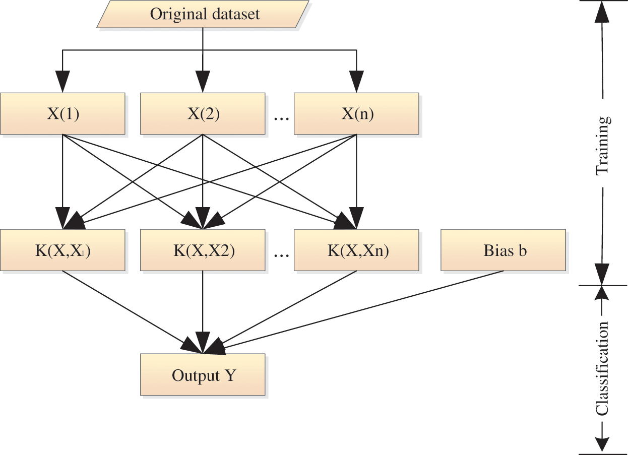
Figure 2: The basic structure of SVM

SVM is essentially a hyper-plane ωTx+b=0 that can separate two types of linearly separable samples to the utmost extent, where the ω∈Rn is the normal vector of the hyper-plane and the b is the bias. In order for that, the distance between the two types of samples 2/‖ω‖ should be maximized. That means the ||ω|| should be minimized. Simultaneously, for handling samples that are not seriously linear separable, a compromise is made to accept misclassification of a few samples with penalty. Then the target function of SVM is described as follows.

minJ(ω)=12ωTω+c∑i=1nξi (2)

S.t.yi(ωTxi+b)≥1−ξi,i=1,2,⋯,n (3)

In Eq. (2): ξi is slack variable for each sample; c is the penalty factor, which decides the fault tolerance of the classifier.

The most crucial characteristic of SVM is that it can transfer nonlinear separable samples in lower dimensional space to linear separable samples in higher dimensional space through using kernel function. The kernel function k(xi,x) is a type of symmetric function obeys the Mercer’s theorem, which corresponds to the inner product of two vectors mapped by certain nonlinear transformation from lower to higher dimensional space. After replacing the inner product with the kernel function, the discriminant function of SVM can be obtained as follows:

f(x)=sgn[∑SVaiyik(xi,x)+b∗] (4)

There are many types of kernel function, including the radial basis function (RBF), the sigmoid kernel, the linear kernel and the polynomial kernel, etc. Literature reviews show that the SVM with RBF has good performance in control chart pattern recognition. Therefore, the SVM with RBF is used as the pattern classifier in this study. The formula of RBF is as follows:

K(x,xi)=exp⁡(−‖x−xi‖/(2σ2))=exp⁡(−g‖x−xi‖) (5)

The parameter g is one of the two hyper-parameters of the SVM with RBF, and the penalty parameter c is the other. Both of them affect the classifying performance of the SVM significantly. Therefore, looking for the best pair of (c,g) is a crucial step in constructing our SVM based pattern recognition model.

2.2.2 CS Algorithm

CS is a new meta-heuristic search optimization algorithm illuminated by the biological characteristics in nature [24]. It combines the simulation of cuckoo birds’ parasitic reproduction process with the Levy flight search principle. In nature, the cuckoo finds its nest position randomly. There are three ideal hypotheses for the cuckoo’s search for the optimal nest: (1) The number of host nests n remains unchanged, allowing the host bird to discover and abandon non-self eggs with probability pa=[0,1] . (2) The best nest with high-quality eggs will be reserved for the next generation; (3) Birds randomly select nests and only lay one egg at a time. Based on the above three ideal conditions, the updated formula for the location and path of the cuckoo’s host nest is as follows:

xit+1=xi(t)+α⊗L(s,λ) (6)

among them

L(s,λ)=λΓ(λ)sin⁡(πλ/2)π(1s1+λ),(s≫0) (7)

In Eq. (6): xi(t) is the i−th nest’s position in t iterations; α is the step length coefficient, usually α>0 , which obeys the normal distribution and controls the step length.

After updating the position by Eq. (6), a random number r(r∈[0,1]) is generated. Comparing r with pa , if r>pa , then randomly update the nest position, otherwise the nest position remains unchanged. The optimal nest position is selected by iterating and updating the nest position continuously.

3  The Recognition Model

The recognition model based on CS-SVM is shown in Fig. 3. It is composed of three modules, namely the data generation module, the CS optimization module and the pattern recognition module. The implementation process of the CS to optimize the hyper-parameters c,g of SVM is the core of this model, which is described in detail as follows:

Step 1: Initialize the basic parameters. When the probability that the host bird finds a non-self bird egg is 0.25, it is sufficient for most optimization problems, so pa= 0.25 was set. The number of iterations is time= 200, the number of nests n= 20, the range of c is [0.01,128] , the range of g is [0.001,128] . The nest position Xi,i∈[1,n] is randomly initialized, and the fitness function is defined as f(x),X=[X1,X2,⋯,Xn]T . The nest position is brought into the fitness function, and the nest with the best fitness position is selected and reserved for the next generation.

Step 2: The position and state of the non-optimal nest are updated by using Eq. (6). The updated nest position is used to recalculate the fitness function value, which is compared with that of the best nest position reserved by the previous generation. When the current value is better, the new nest position is reserved to replace the old best nest.

Step 3: After the nest position is updated, the random number r is compared with pa . Then the fitness function is used to test whether the updated nest position is better in comparison with the previous generation to determine the new optimal nest position.

Step 4: If the maximum number of iterations or required accuracy is reached, the obtained optimal bird nest position is accepted as the global optimal solution; otherwise, turn back to step 2 and continue to iterate and update.

Step 5: Output the position of the global optimal nest, namely the best hyper-parameters c,g .

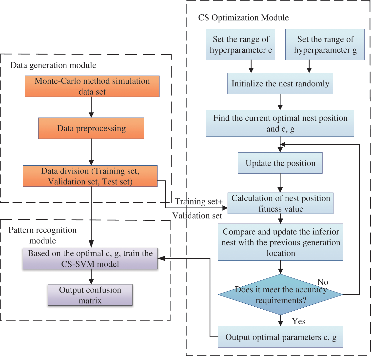
Figure 3: Recognition model based on CS-SVM

4  Simulation Experiments

4.1 Experimental Environment and Data

In order to verify the performance of the proposed model, which is established through programming in the MATLAB2018, and hereinto, the SVM is realized by the Libsvm toolbox. Then, some simulation experiments with this model are carried out in the MATLAB2018. The performance indicators of the computer used are CPU2.4GHZ, RAM12.0G. Following the conventional research methods in this field, eight types of basic CCP sample (as described in 2.1) of AR (1) process are generated by Monte carol simulation method. These samples are divided into three mutually exclusive sets, including the training set, the validation set and the test set. The number of samples for each pattern in each set is shown in Tab. 1. To reflect the diversity of abnormal amplitudes in actual processes, exception parameters of the abnormal patterns take values within certain specific range. The parameter choices of all patterns are shown in Tab. 2. With reference to other literatures, the dimension of the pattern sample vector (that is, the width of the online recognition window) is set equal to 32.

Table 1: Sample numbers

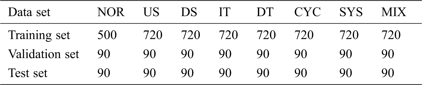
Table 2: Parameter settings of the eight patterns

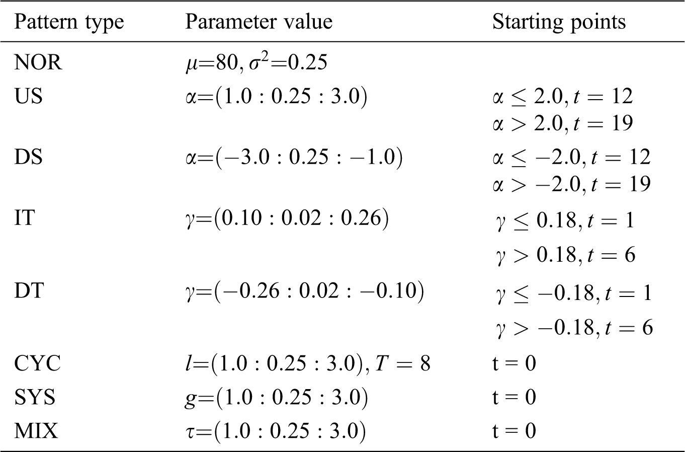
For the patterns of US, DS, IT, and DT, different starting points of exception are set for different abnormity amplitudes. Small amplitudes have smaller abnormal starting points, for example, in US, t=12 when α≤2.0 . The purpose is to make the abnormal pattern samples with smaller amplitude contain more information, so that the trained model can identify which more easily.

4.2 Optimization Process of CS-SVM

In each iteration of the CS, the CS-SVM model is trained after being given the hyper-parameters, and calculated recognition accuracy with the verification set. The result is taken as the fitness value. Without loss of generality, the hyper-parameters are optimized when the autocorrelation coefficient ϕ=0.5 and also used for other autocorrelation levels. Five times of optimization have been carried out, and the corresponding convergence procedures are shown in Fig. 4. All of them converge rapidly within 20 iterations, and reach the fitness value of 98.33%. The earliest one converges at the 11th generation, which get c = 4.9934, g = 0.3675. Hence, this couple of values are set as the model’s hyper-parameters.

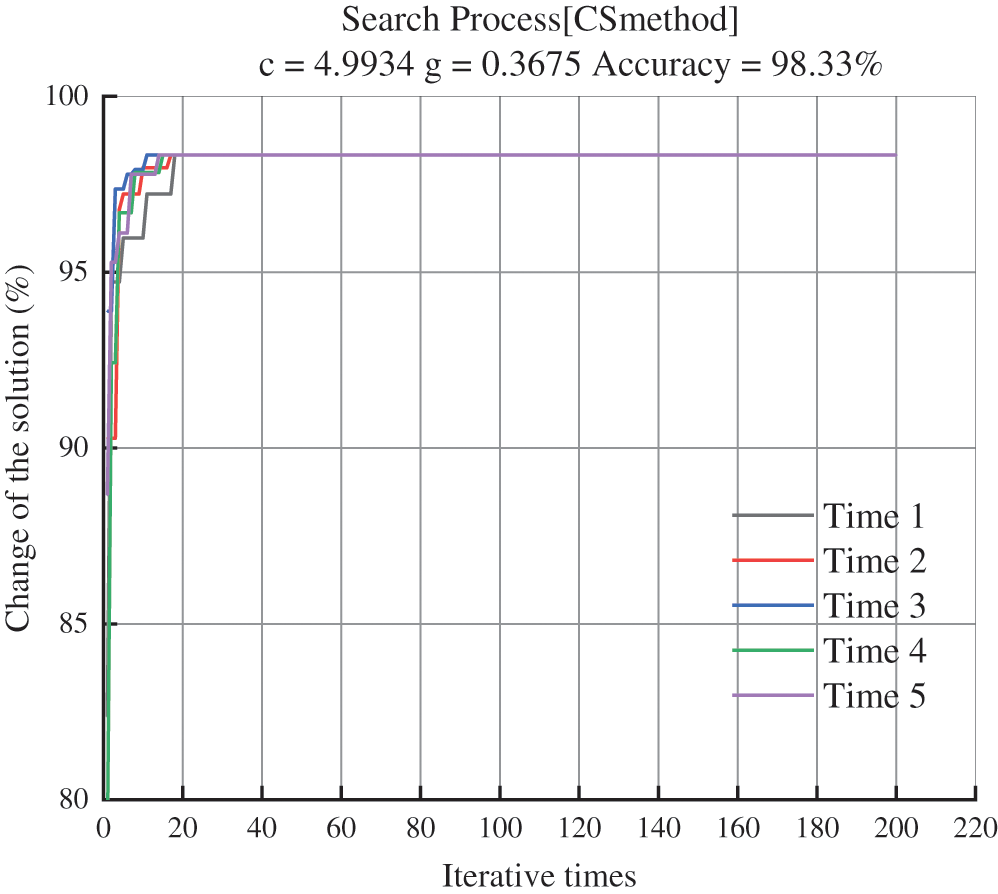
Figure 4: Iteration of CS-SVM model

4.3 Recognition Accuracy Test

Recognition accuracy test of this model is carried out on the test set. For the case of ϕ=0.5 , the confusion matrix of the eight types of pattern is obtained, as shown in Fig. 5. It shows that the recognition accuracies of seven patterns achieve higher than 98%. Among them, the DT pattern gets the highest accuracy, reaching 100%. But the MIX pattern gets a relatively low accuracy, only at 80%. The reason is that the MIX pattern essentially obeys normal distribution, which is different from the NOR pattern only in mean and variance, so that easy to be misjudged as the NOR pattern. The average accuracy of the eight types of pattern reaches 96.25%.

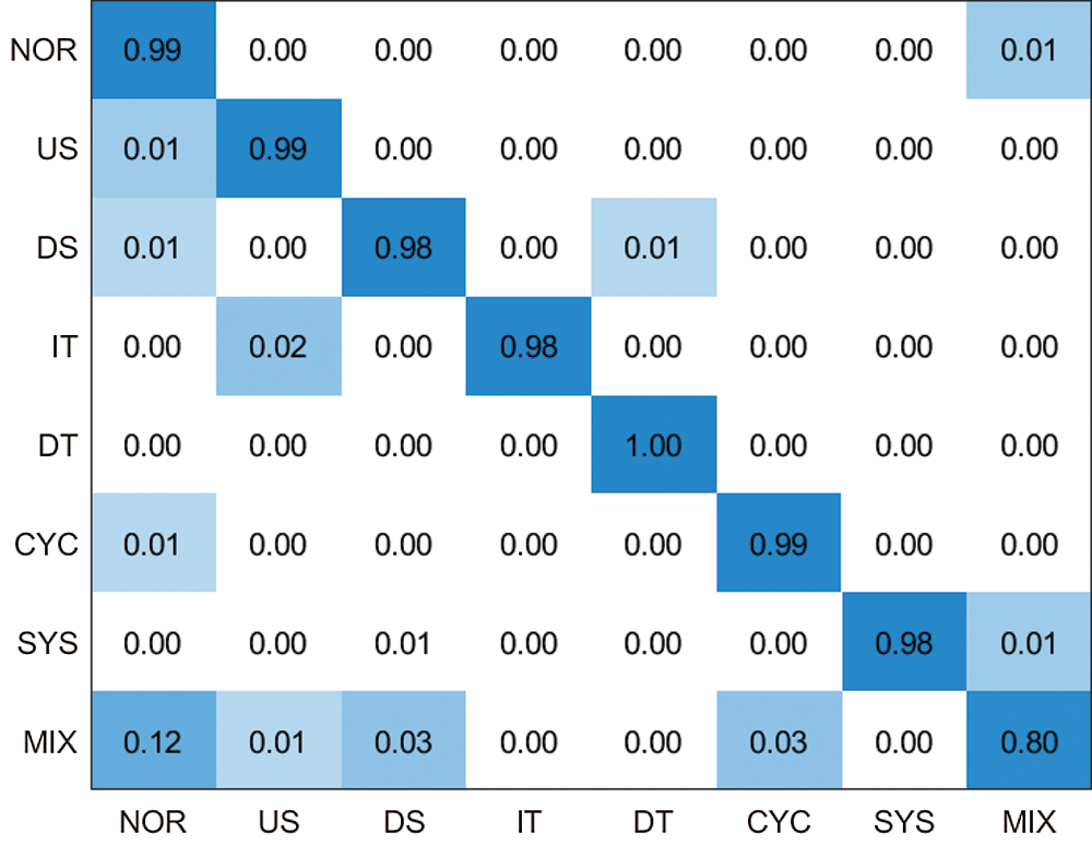
Figure 5: Confusion matrix for the case of ϕ=0.5

The average accuracy of processes with some other different level of autocorrelation coefficients ( ϕ∈{−0.9,−0.7,−0.5,−0.3,−0.1,0,0.1,0.3,0.5,0.7,0.9} ) are shown in Fig. 6. It can be seen that all of these accuracies are above 95%, and the accuracies of the positive correlation cases are slightly higher than those of the negative ones. In addition, the accuracy reaches 98.13% in the case of ϕ=0 , which means that the process is not affected by autocorrelation. These results mean that this model can handle processes with different levels of autocorrelation.

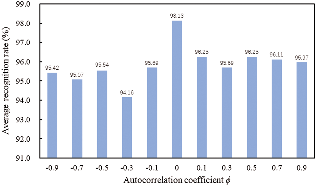
Figure 6: Recognition accuracy in different level of autocorrelation

4.4 Comparative Experiment

In order to further verify the superiority of this model, a comparative experiment was carried out based on the same data sets. The chosen comparative objects are the model based on SVM optimized by particle swarm optimization (PSO-SVM) and the model based on SVM optimized by genetic algorithm (GA-SVM). The reason is that both PSO and GA are intelligent optimization algorithms, which are often used to optimize the hyper-parameters of SVM. Five times of optimization are conducted for the case of autocorrelation coefficients ϕ= 0.5, and then the average convergence time and average recognition accuracy on the test set are used as the comparative indicators. The main parameter settings of these models are shown in Tab. 3. The comparative results are shown in Fig. 7.

Table 3: The setting of main parameters

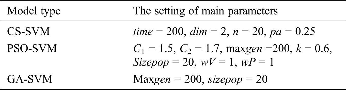
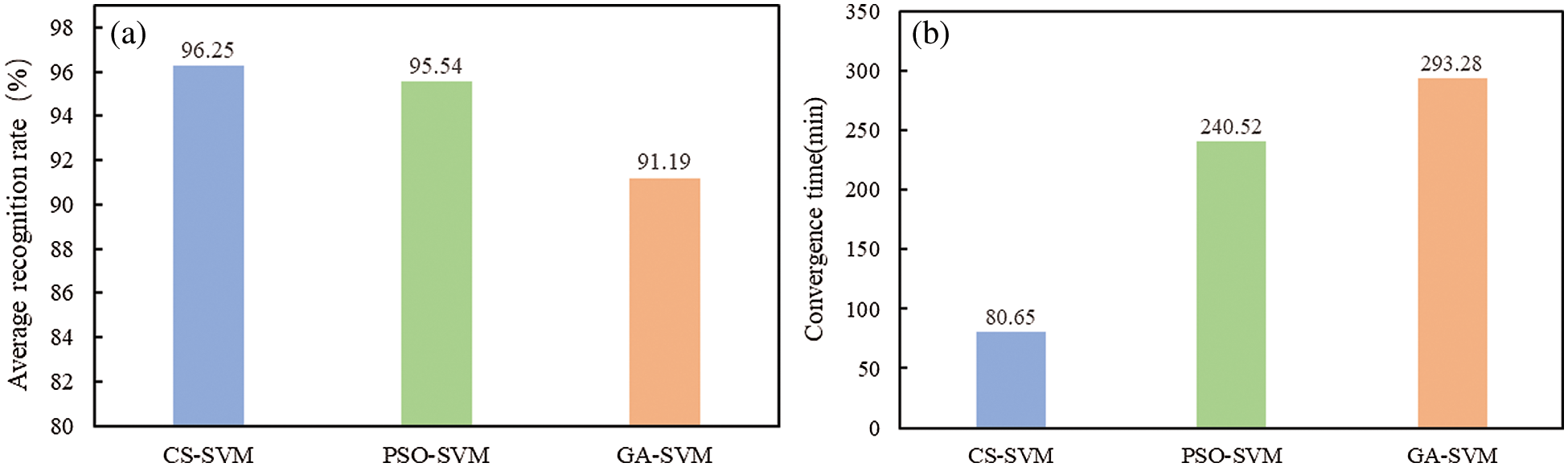
Figure 7: Performance comparison of model optimized by three algorithms. (a) Comparison of recognition accuracy and (b) Comparison of convergence time

It can be seen from Fig. 7a that the proposed model obtains the highest average recognition accuracy with c= 4.9934 and g= 0.3675. The PSO-SVM based model takes the second place (the accuracy is 95.54%) with c= 98.4233 and g= 0.0366. The GA-SVM based model get the lowest accuracy (91.19%) with c= 100.4169 and g= 0.0039. It can be seen from Fig. 7b that the proposed model takes the shortest time (80.65 minutes) to converge, which is much less than those of the PSO-SVM based model (240.52 minutes) and the GA-SVM based model (293.28 minutes). Thus, we believe that the CS-SVM based model we proposed has the best abnormal pattern identification performance for autocorrelation process in comparison with the two comparative objects.

4.5 ARL Measure

Average run length (ARL) is a key indicator of the online performance of control chart or other process anomaly detectors. ARL can be measured through simulation method. The usual practice is to simulate lots of data streams first, and then fetch data from each data stream with a sliding window, till a normal pattern sample is misrecognized as abnormal (ARL0) or an abnormal pattern is identified (ARL). In this study, 3000 in-control data streams and 3000 × 9 × 7 out-of-control data streams are separately generated for each autocorrelation level. The ARL0 reflexes the probability of occurrence of the type I error in the model, and should be controlled as close as possible to the theoretical value (370 for the univariate process) before measuring ARL. For that reason, the try and error method is applied, i.e., the number of the NOR sample in the train data set is adjusted according to the achieved ARL0 value till it reaches slightly higher than 370. In addition, the SRL (standard deviation of ARL) is also calculated to measure the stability of ARL performance.

In order to verify the online performance of the proposed CS-SVM based model, an SVM based model in reference [15] is chosen as a comparative object, and the comparative data are obtained from its Tab. 3. The Tab. 4 shows the comparison of the average ARL values and the average SRL values of the proposed model and those of the comparative object, which are calculated for different abnormity magnitudes of each abnormal pattern under different level of autocorrelation. For comparative purpose, the ARL value of the proposed model which is not lower than that of the comparative object is highlighted in bold in the Tab. 4.

Table 4: Comparison of ARL and SRL values between the CS-SVM based model and the referenced SVM based model

It can be seen that the proposed model performs better for the US, DS, IT and DT pattern as ϕ≥0 , and better for the SYS and MIX pattern as ϕ<0 . However, the aggregated average ARL values indicate that the proposed model takes an advantageous position, since it obtains lower ARL values than those of the comparative object for 8 of the 11 levels of autocorrelation. At the same time, the aggregated average SRL values of the proposed model are very close to those of the comparative object. In that, the proposed model can be regarded as having an acceptable online performance.

5  Conclusion

This study uses CS to optimize the two hyper-parameters of SVM (CS-SVM), and then based on which to establish a recognition model for abnormal patterns in autocorrelation process. A series of simulation experiments have been conducted to test the performances of this model. The experiment results show that the established model can achieve higher recognition accuracy in comparison with the model based on SVM optimized by the PSO or the GA. In the meantime, it takes much less time to optimize the hyper-parameters for this model. That means this model has higher training efficiency, considering that the parameter optimization procedure is involved in the training process. Furthermore, the model shows good recognition accuracy for each tested autocorrelation level (whether positive or negative autocorrelation), indicating its broad applicability. At last, the ARL values of the model at different autocorrelation levels are measured, which are generally better than those of the comparative model from the reference. That indicates the model also possesses an acceptable online performance. Identification of abnormal patterns in autocorrelation process is still in the exploratory stage, and the proposed model provides a new way for it. Currently, we have verified the model’s effectiveness through simulation experiments. Testing the model’s effectiveness for other types of autocorrelation processes except AR (1) and studying how to use it in the actual manufacturing process will be our next work.

Acknowledgement: I want to take this chance to thanks my tutor----Bo Zhu. In composing this paper, he gives me much academic and constructive advice and helps me correct my essay. Besides these, he also allowed me to do my teaching practice. At the same time, I want to thank my friends Chunmei Chen, Kaimin Pang and Yuwei Wan. They participated much in this research. Finally, I’d like to thank all my friends, especially my three lovely roommates, for their encouragement and support.

Funding Statement: This research was financially supported by the National Key R&D Program of China (2017YFB1400301).

Conflicts of Interest: The authors declare that they have no interest in reporting regarding the present study.

Appendix A. Mathematical Expressions of Eight CCPs

In this research, the Monte Carlo simulation approach was used to generate the required sets of CCPs for training, test, and validation data set. The CCP herein is expressed in a general form that consists of the process mean, the common-cause variation, and a special disturbance from specific causes.

Process Simulator

Xt=μ+εn+dt

where

μ = process means in the controlled state

εn = common-cause variation at time t (by the polar method), following a normal distribution with zero mean and standard deviation σ , where

σ = process standard deviation when the process is in control and was fixed at 0.25 in this research

dt = special disturbance at time t

Normal (NOR): dt=0

Shift (US/DS): dt=λ×α

where

λ = parameter to determine the position of shifting ( λ=0 before shifting; λ=1 after shifting)

α = displacement of mean in terms of σ

Trend (IT/DT): dt=γ×t

where

γ = trend slope in terms of σ

Cycle (CYC): dt=l×sin⁡(2πtT)

where

l = cycle amplitude in terms of σ

T = cycle period (T = 8 in this research)

Systematic (SYS): dt=g×(−1)t

where

g = magnitude of the systematic pattern in terms of σ , determining the fluctuations above or below the process mean

Mixture (MIX): d(t,p)=τ×(−1)h

where

p = a random number ( 0<p<1 )

τ = magnitude of the mixture pattern in terms of σ , determining the fluctuations above or below the process mean

h = 0 if p<τp , 1 if p>τp

This work is licensed under a Creative Commons Attribution 4.0 International License, which permits unrestricted use, distribution, and reproduction in any medium, provided the original work is properly cited.