Intelligent Automation & Soft Computing DOI:10.32604/iasc.2021.016752
Article

Effect of Load on Transient Performance of Unearthed and Compensated Distribution Networks

Nehmdoh A. Sabiha*and Hend I. Alkhammash

Department of Electrical Engineering, College of Engineering, Taif University, P.O. Box 11099, Taif, 21944, Saudi Arabia
*Corresponding Author: Nehmdoh A. Sabiha. Email: n.sabiha@tu.edu.sa
Received: 10 January 2021; Accepted: 04 March 2021

Abstract: The maximum temperature that cable insulation can withstand determines the maximum load that the cable conductor can carry, which is called cable ampacity. However, a temperature far from this value under normal load conditions affects the transients due to earth faults in the distribution network. Accordingly, error estimation in the fault location occurs, and the smart grids do not accept such errors. Considering heterogenous unearthed and compensated distribution networks, the temperature rise in different underground cables is estimated under different load conditions. These loads are full load, three quarters (3/4) load, one half (1/2) load, and one quarter (1/4) load. The generated heat in the cable conductor due to these loads is calculated, and the corresponding temperatures are estimated. The distribution of the temperature across XLPE is ascertained using COMSOL Multiphysics by an interface of heat transfer in solids. The impact of these temperature increases on the XLPE relative permittivity is investigated. Moreover, the impact of relative permittivity on the transients due to the earth faults is investigated. Time and frequency domains of the faulted currents are investigated to determine the effect of load. The effect of the load on the arrival time of traveling surge created due to the fault event is measured using a voltage transducer at the main busbar, and evaluated. Accordingly, the time arrival deviations due to effect of load produce an undesired error in the fault location determination using traveling wave principles. Simulations of the fault cases are implemented in ATPDraw, and Matlab is used to extract the surge arrival time. This work contributes to highlighting the errors involved in the fault location algorithms using network transients due to network service operation at different load conditions.

Keywords: Earth faults; heterogenous unearthed and compensated distribution networks; relative permittivity; temperature distribution; XLPE cables

1  Introduction

Medium-voltage power networks are geographically widely distributed. Accordingly, they are subjected to faults, where the most common fault type is the phase to ground one (called an earth fault). Earth fault currents are extremely high in earthed networks due to the earth loop availability through the connected neutral point of the main transformer to the earth. Conversely, the fundamental earth fault currents are low in unearthed networks since the earth loop is through the capacitances of overhead sections and underground cables [1,2]. To diminish the earth fault currents, compensated networks are applied where the Petersen coil is connected at the neutral point of the main transformer. This coil is used to compensate for the network capacitance. The main advantage of the unearthed and compensated networks is that they enhance the service continuity during earth faults. Such networks are common in Nordic countries.

Earth fault detection in the unearthed compensated networks depends on monitoring the neutral voltage or evaluating the residual voltage that is three multiples of the zero sequence voltage. However, the distribution networks are lateral, which produces challenges for the selectivity protection functions and fault location algorithms. This is because these functions are based on fundamental currents that are small during earth faults in unearthed and compensated networks. Hence, the transients are the main tools used to apply selectivity and fault location algorithms [3–8].

Transients in the unearthed and compensated networks are characterized into discharge and charge transients, as well as traveling waves [2,3,9]. Once an earth fault occurs, traveling waves are generated and travel through the network laterals until they reach measuring points. Such traveling waves are called passive traveling waves, and they are evaluated to estimate the fault distance. The other traveling waves that are applied to the fault network to also estimate the fault distance are active traveling waves, and they utilize external devices [3]. Both passive and active traveling waves are completely dependent on the overhead and underground cable parameters and configurations. Unfortunately, these parameters are affected by the conductor temperatures, which are influenced by the current carrying load. These parameters are the resistances, inductances, and capacitances, which comprise the main representation of the overhead and underground cable lines. Thermal stress negatively affects the electrical and mechanical properties of both overhead lines and underground cables. Conductor power losses increase with increasing temperature. Increasing temperature also negatively impacts mechanical properties, as tensile strength decreases and sage of the overhead lines is increased [10]. Considering increasing temperature, both breakdown voltage and dielectric constant are decreased with aging time. However, the dielectric loss is increased. Thermal cable surroundings play a very important role in temperature control because of their responsibility for heat dissipations, and therefore the cable rating is impacted by the boundary or environmental temperature, as addressed in [11].

The discharge transients in unearthed and compensated networks are created by earth faults where the earth capacitances are discharged and produced high frequencies in the network. However, the charge transients are created after the discharge transients, and are produced by charging process of the healthy phases. The charge transients have other frequencies, but they are lower than the discharge frequencies. Frequencies of discharge or charge processes have been utilized to estimate the fault distance [9]. Similarly, they are affected by the overhead and underground cables configuration and parameters that are influenced by the conductor temperatures throughout the network’s operation. Current-carrying cable conductors generate heat, affecting the cross-linked polyethylene XPLE characteristics. Based on the rating of the cable currents, the dielectric and electric characteristics of the insulator are changed due to the temperature rise across insulators.

A few publications have focused on ampacity calculations of the underground cables [11–13]. For boundary temperature restrictions, ampacity was calculated for submarine cables [11]. In [12], the advantages that motivate the great depth of installing cable underground were highlighted, the ampacity was calculated, and the impact of depth on ampacity determined. However, this study was restricted to steady state conditions, and achieving the ideal depth is difficult in many situations. Installation requirements and reasonable application have to be well considered to obtain an accurate ampacity [13]. Using different methods for evaluating the ampacity for a certain cable with the same conditions leads to different results [14]. To economically optimize cable installation, ampacity must be considered along with cost [15]. Furthermore, temperature rise affects the electrical characteristics of XLPE: the permittivity of the XLPE decreases with increasing temperature, which negatively affects the quality of the insulation [16]. A continuous high temperature affects insulation since it leads to thermal aging [17]. Thermal parameters of the insulation cable determine the cable ampacity [18]. Changing the dielectric constant of the XLPE leads to changing the current carrying conductor characteristics under fault conditions. Considering short-circuit loading as an emergency condition, accelerated thermal aging and the lifetime of the cable insulation were investigated under a very high temperature [19]. For maximizing the current of the cable conductor, the cable system was optimized [20]. Therefore, during transients, attention toward both unearthed and compensated networks for Petersen coil performance is required.

In this paper, heterogenous unearthed and compensated distribution networks are utilized to evaluate the loading effect on network transients. The temperature rises across the XLPE of the underground cable under different load conditions are estimated. Then, the corresponding relative permittivity of XLPE is investigated based on the temperature. The transients due to the earth fault in both networks are investigated under different load conditions. The impact of relative permittivity and different load conditions on the earth fault currents and the earth fault location determination are declared. This study confirms the importance of considering load effects on the transients in distribution networks.

2  Research Methodology

To estimate the effect of loading issues on earth fault currents for unearthed and compensated distribution networks, we consider several procedures:

1.   Estimate the conductor losses for each cable after measuring the distributed currents under different load conditions using ATPDraw software. These load conditions are considered in this study: a full load, three-quarters (3/4) load, one half (1/2) load, and one-quarter (1/4) load.

2.   Determine the conductor temperature for the cables using COMSOL Multiphysics and based on the losses determined in step 1 as a heat loss applied to the conductor.

3.   Estimate the corresponding relative permittivity (εr) using the reported curve in [21] of experimental temperature-dependent relative permittivity.

4.   Measure the fault current in the unearthed network while considering the relative permittivity reported in the cable datasheet [22] and the aging cable’s condition.

5.   Measure the fault current and the corresponding transients in unearthed and compensated networks under different load conditions.

These procedures are shown in the flowchart in Fig. 1.

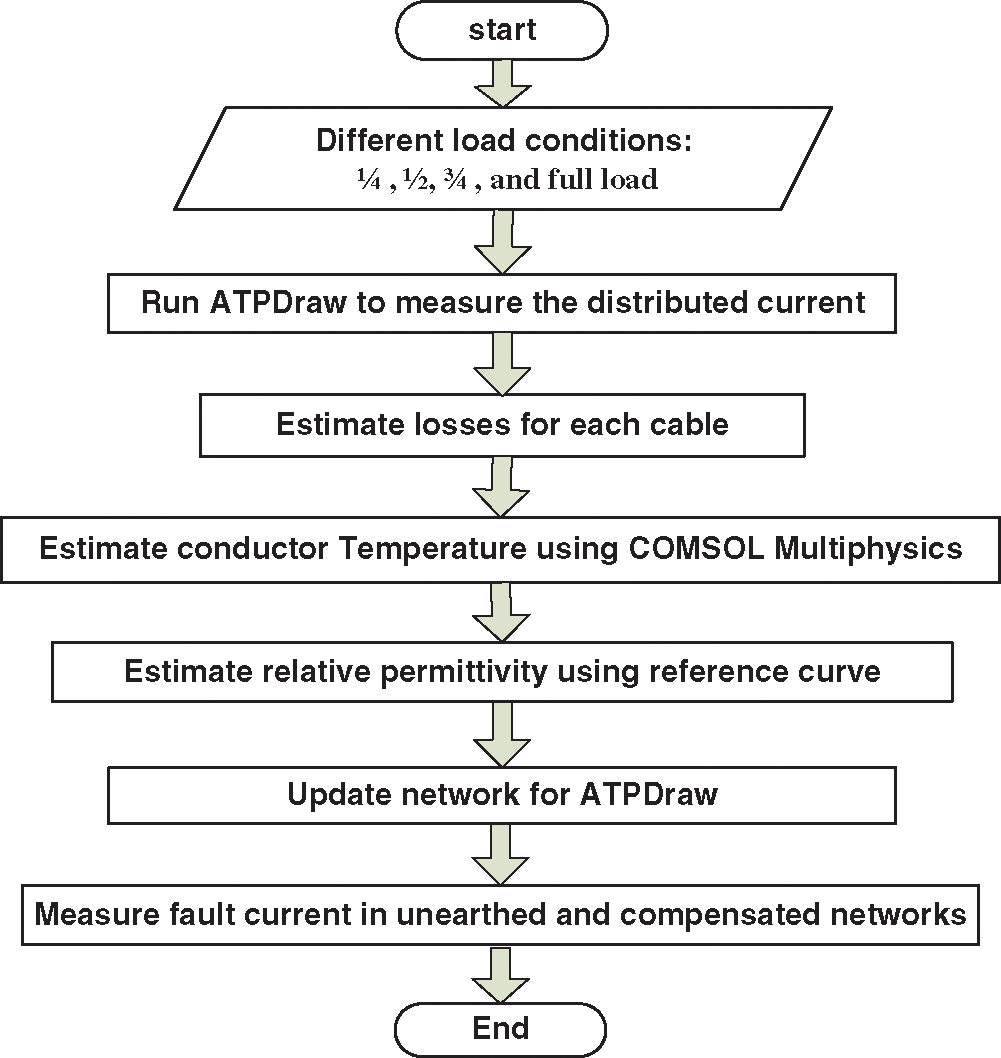
Figure 1: Flowchart for the study procedures

3  Simulated System: One-line Diagram, ATPDraw Circuit, and COMSOL

Fig. 2a shows the electric distribution network rated at 20 kV, 68 MVA, and the network contains four distribution feeders. A resistor–capacitor (RC) transducer of 100 Ω and 0.01 μF is used to measure the traveling waves due to earth fault. The network is heterogeneous type, and the total XLPE cable length is 40% of the total network length. The configurations of the overhead tower and underground cable are shown in Figs. 2b and 2c, respectively, and the dimensions are reported in [3]. The underground cables are represented on the basis of single core cables in the arrangement shown in Fig. 2c. Each cable section is installed 1.3 m underground, the conductor resistivity is 2.84 × 10−9 Ω.m, the cross-section area is 185 mm2, the insulation thickness is 0.015 m, the sheath thickness is 0.003 m, and the outer insulation thickness is 0.01 m. The relative permittivity of the XLPE is initially assumed to be 2.3. The network is considered unearthed and compensated using the Petersen coil. Fig. 3 shows the equivalent circuit of the earth fault current, where the source is the phase voltage, Rf is the fault resistance, C is the summation of earth capacitances, Rd is the dielectric resistance, and L is the added compensation coil (Petersen coil) placed at the neutral point (see Fig. 2). We simulate two networks by considering two earthing concepts. The first one is the unearthed network, and the second one is the compensated network. In order to compensate for the earth fault current in the network, the Petersen coil is added to produce parallel resonance with the capacitance (see Fig. 3). This compensation coil is found as 360 mH to compensate the earth fault current.

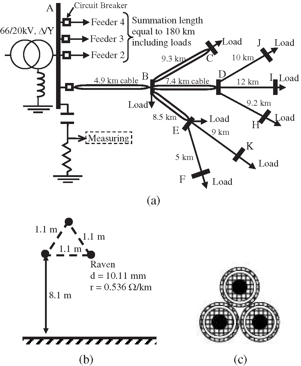
Figure 2: Simulated distribution network. (a) Modified suburban distribution feeder. (b) Configuration of overhead tower [3]. (c) Arrangement of underground cable [3].

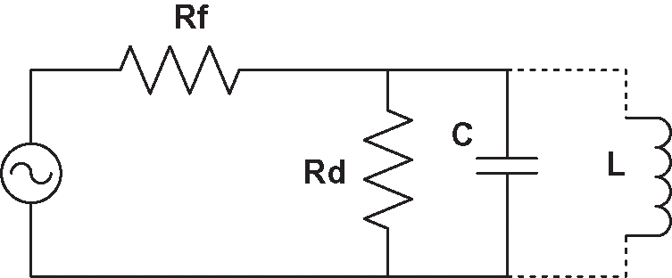
Figure 3: The equivalent circuit of the earth fault current

By simulating the unearthed and compensated distribution networks using ATPDraw, an earth fault occurs at busbar E, shown in Fig. 2, when the networks are unloaded. Fig. 4 shows the corresponding earth fault currents considering these two earthing concepts. Fig. 4a shows the time-domain performance, and Fig. 4b shows the corresponding fast Fourier transform (FFT)-based frequency analyses considering the reference permittivity of 2.3 reported in the cable datasheet [22]. The simulated fault current is directly measured by monitoring the current through the fault switch itself in the ATPDraw circuit, and there is no need to add any transducer element. As shown in the zoomed-in diagram in Fig. 4a, there are discharge/charge currents producing transients due to the fault event at 10.5 ms. The instantaneous maximum current is -1116 A for both unearthed and compensated networks. As confirmed by Fig. 4.b, the fundamental value of the fault current (at 50 Hz) is 123 A (rms value) for the unearthed network; however, the fundamental current of the compensated network is 10.06 A (rms value). We can observe two periods from the earth fault current waveforms shown in Fig. 4a. The first one is the transient period, where the behaviors of the two networks are approximately close. During this fault period, the compensation coil represents an open circuit as the transient period contains high frequencies. Therefore, the transients in the compensated network look like the transient behavior of the unearthed network. However, the fundamental fault currents are different in the two networks during the steady state fault period (the second fault period), which is after the transient period. Such earth fault behaviors, in either the transient or steady state in the unearthed or compensated networks, depend on the network’s electric parameters, i.e., mainly the network’s capacitances and inductances. The network’s capacitances are the overhead and underground capacitances. It is common for underground cables to have higher capacitances, and these capacitances depend on the cable dimensions and permittivity. However, the cable permittivity is influenced by temperature, which is affected by carrying cable currents.

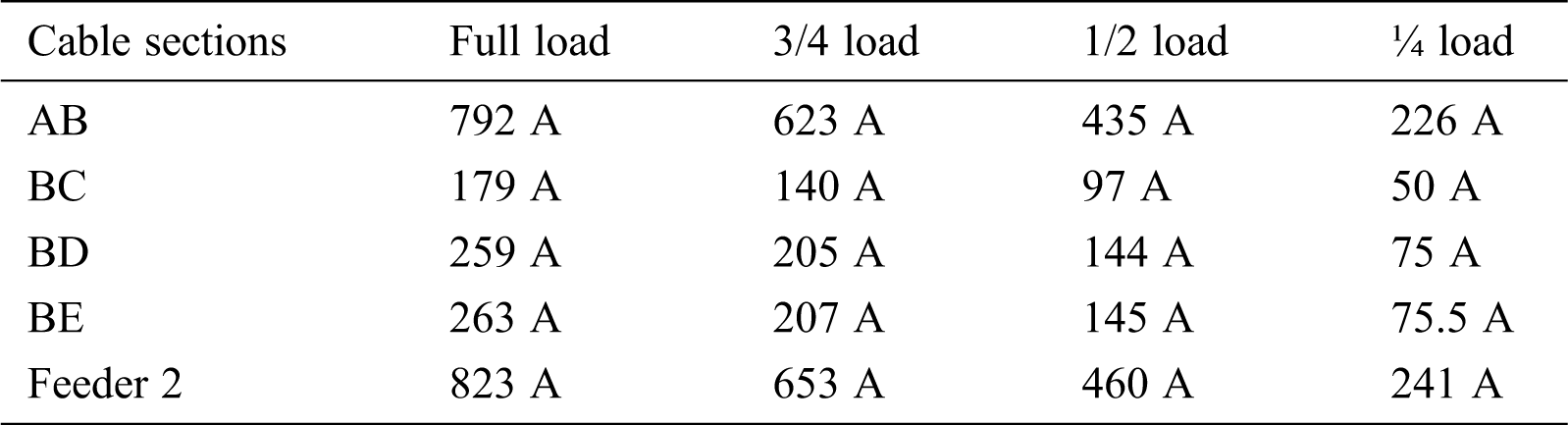
Tab. 1 shows the load currents through the distribution network (Fig. 2). The results in this table are for a full load, three quarters (3/4) load, one half (1/2) load, and one quarter (1/4) load. These currents are utilized to estimate the thermal distribution through the underground cables and therefore the cable relative permittivity factor; this is further discussed in the following section. For the simulated network, the loads are changed in the same manner and with the same load conditions. First, the full load impedance is calculated for each network branch at the 400 V level. Then, these impedances are doubled to produce the half-load condition. Similarly, the load impedances were computed for the ¼ load and ¾ load conditions.

Table 1: Cable loading currents distribution measured by ATPDraw (peak values).

4  Modeling Effect of load on Cable Parameters

4.1 Calculating the Cable Temperatures with Load Effects

Different load conditions lead to different amounts of heat generated in the conductor; this heat is dissipated through the cable insulation and the soil environment. COMSOL Multiphysics [23] is used to accurately model the temperature distribution across the XLPE while considering different load currents. For each load current, thermal equilibrium is achieved where the stationary study is implemented with a heat transfer interface in COMSOL Multiphysics. The heat transfer in solids is represented by:

ρCp(∂T∂t)+ρCpu.∇T+∇.q=Q (1)

q=−k∇T (2)

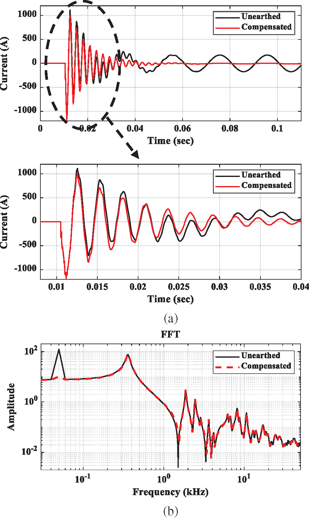
Figure 4: Comparison between the earth fault currents of unearthed and compensated networks. (a) Time domain comparison. (b) FFT-based frequency comparison

where ρ is the density (kg/m3), and is 1300, 8960, and 1600 kg/m3 for XLPE, copper, and soil, respectively. Cp is the heat capacity at constant pressure (J/kg · K), and is 1850, 385, and 1180 J/(kg · K) for XLPE, copper, and soil, respectively. T is the absolute temperature (K), u is the velocity field (m/s), q is the heat flux by conduction (W/m2), and Q is the heat source (W/m3) that is a function of the current-carrying conductor, the conductor’s cross-section area, and the conductor’s material.

As heat transfer in solids is considered as a physics interface in COMSOL, the conductor heat loss (W) based on Equation (3) corresponds to the above-mentioned loads (full load, ¾ load, ½ load, and ¼ load):

W=I2ρclA(1+αc(Δθ)) (3)

where I is the current-carrying conductor (load current), ρc is the conductor resistivity, l is the conductor length, A is the cross-section area of the conductor, αcu is the copper temperature coefficient at the reference temperature, and Δθ is the difference in temperature between the ambient temperature and the reference temperature (35°C and 20°C, respectively). These calculated heat losses are injected into the conductor to simulate the thermal effect of the loading current. Then, the temperature distribution across the XLPE is estimated as shown in Fig. 5 for the investigated loads (Tab. 1). This figure shows that the maximum temperature is recorded in FEEDER 2 for all load conditions and reaches 72°C under full load conditions. A slight change between FEEDER 2 and SECTION AB is noticed. However, a significant difference is found in temperatures of the main section AB in the faulted feeder in the network shown in Fig. 2 and the other cable sections BC, BD, and BE. Other sections record a slight change in temperature. This ensures the effect of the load currents carried through the network on the cable section temperature distribution. These changes in temperatures affect the dielectric constant (permittivity) of the XLPE. For more practical information regarding the underground cables, the maximum allowable temperature of the underground cable is generally 90°C or 105°C for medium-voltage networks [13]. Furthermore, the XPLE cable can carry large currents under different conditions: 90°C for normal operation, 130°C for emergency operation, and 250°C for short circuits [24].

4.2 Calculating the Cable Permittivity and Effect of Load

The experimental temperature-dependent relative permittivity published in [21] for XLPE is fitted to attain the value of relative permittivity under different temperatures. The following fitted equations are obtained as a function of insulator temperature (T) in °C:

εr={−147.2+T−64.15+0.405TT≤100∘C2176T2+1.7T>100∘C (4)

Considering the first part of the above equation for T ≤ 100°C as well as the investigated temperatures under different load conditions shown in Fig. 5, the relative permittivities of XLPE are extracted and listed in Tab. 2. The relative permittivity decreases with increasing load current. This decrease in XLPE permittivity produces an increase in the electric field across the insulator, which accelerates the deterioration of the insulator. The electrostatics physics interface is used to describe the electric field in XLPE insulation in the current study, where the applied voltage is considered as 16.33 kV over the cable conductor. The electric field is evaluated using Gauss’ law:

−∇.(ε0∇V−P)=ρe (5)

where ε0 is the permittivity of vacuum (F/m), P is the electric polarization vector (C/m2), and ρe is the space charge density (C/m3). Fig. 6 displays the electric field stress with increasing load. The load increases the temperature, which reduces the relative permittivity, and this permittivity increases the electric field.

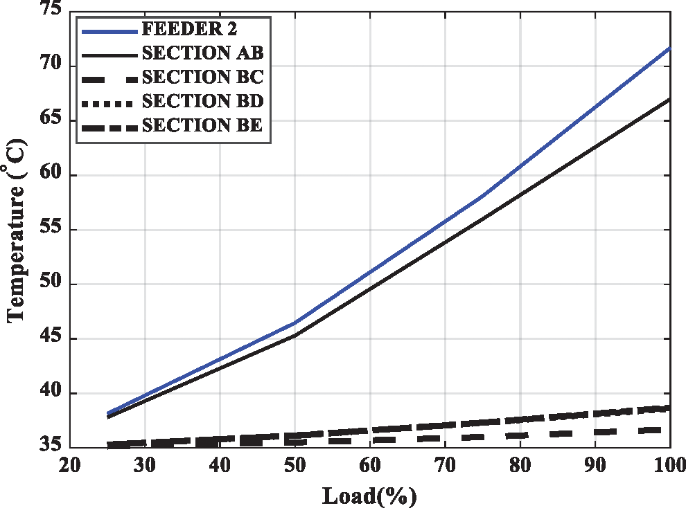
Figure 5: Temperature across XLPE under different load conditions

Table 2: Corresponding XLPE relative permittivity

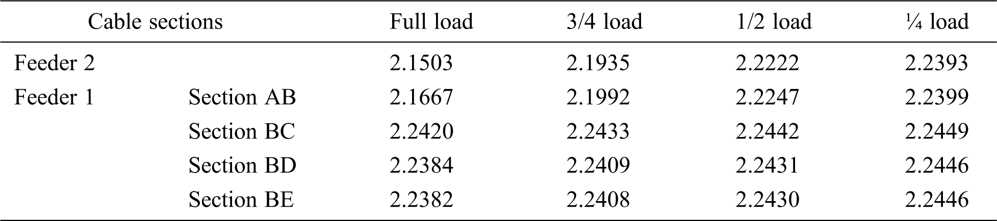
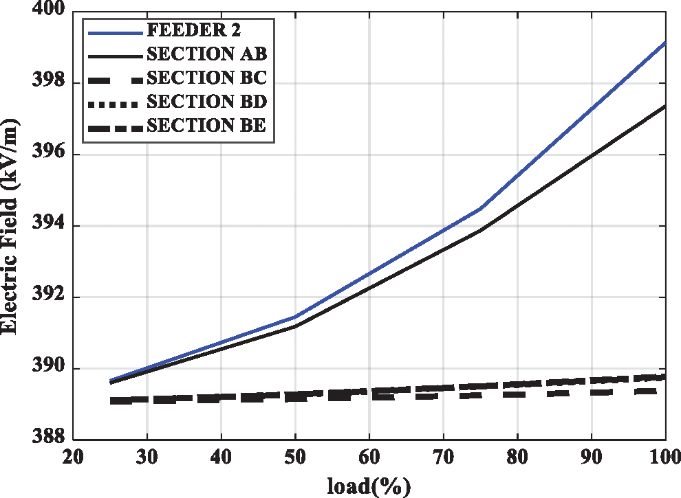
Figure 6: Electric field stress due to load changes

5  Effect of Relative Permittivity of Underground Cables on the Transients of Unearthed Distribution Networks

In this section, we use the value of 1.8 relative permittivity of XLPE, which is observed when the cable is aged [21]. This is the minimum relative permittivity value. However, the 2.3 relative permittivity value is also used because it is reported in the cable datasheet [22]. These two values are utilized to show the effect of the relative permittivity values on the network transients.

5.1 Fault Current Waveforms and FFT

Fig. 7 shows the relative permittivity effect on the earth fault currents for the unearthed power distribution networks. As aforementioned, the fault point is at busbar E in the network shown in Fig. 2. As shown in Fig. 7.a, there is a significant difference in the fault current due to the change in relative permittivity of the underground cable, i.e., from the datasheet value of εr = 2.3 to the value corresponding to age εr = 1.8. As discussed in the previous section, increasing the cable temperature reduces the relative permittivity. Under the worst condition of cable aging, the relative primitivity of the cable insulation was found to be εr = 1.8, as reported in [23]. FFT analyses presented in Fig. 7.b confirm the changes in the fault currents due to the changes in the cable insulation permittivity from εr = =2.3 to εr = 1.8. These results depict the temperature effect on the transients of the distribution networks.

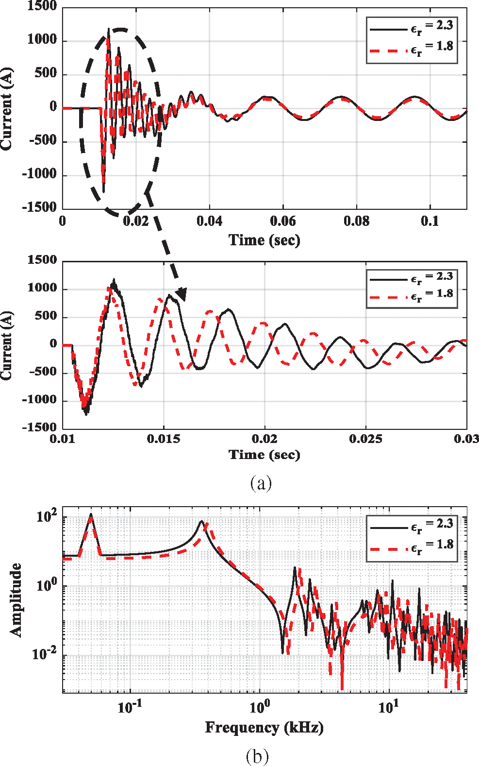
Figure 7: Relative permittivity effect on the earth fault currents of unearthed networks. (a) Time domain comparison. (b) FFT-based frequency comparison

5.2 Extracted and Measured Transients Using Voltage Transducers

Fig. 8 shows the effect of relative permittivity on the measurements taken using the RC transducer (see the network in Fig. 2) for the earth fault in the unearthed power distribution networks. For the results in this figure, the relative permittivity values are considered as εr = 2.3 and εr = 1.8. As depicted in Fig. 2, the RC transducer of 100 Ω and 0.01 μF is utilized to measure the voltage transients due to the earth fault event at 0.0105 s in the unearthed network for different load conditions. Fig. 8 shows these measurements. The waveforms are the residual voltage measured over the resistor of the RC transducer. The residual voltage is the summation of the phase voltages. This is suitable for monitoring earth faults. The voltage over the resistor is the proportional derivative of the busbar voltage where the RC transducer is installed. The proportional factor depends on the RC transducer parameters. Hence, Fig. 8 shows the proportional derivative of the residual voltage at busbar A due to earth fault in the network. The traveling waves of the earth fault and the corresponding reflected surge in the network are extracted using the derivative of the residual voltage.

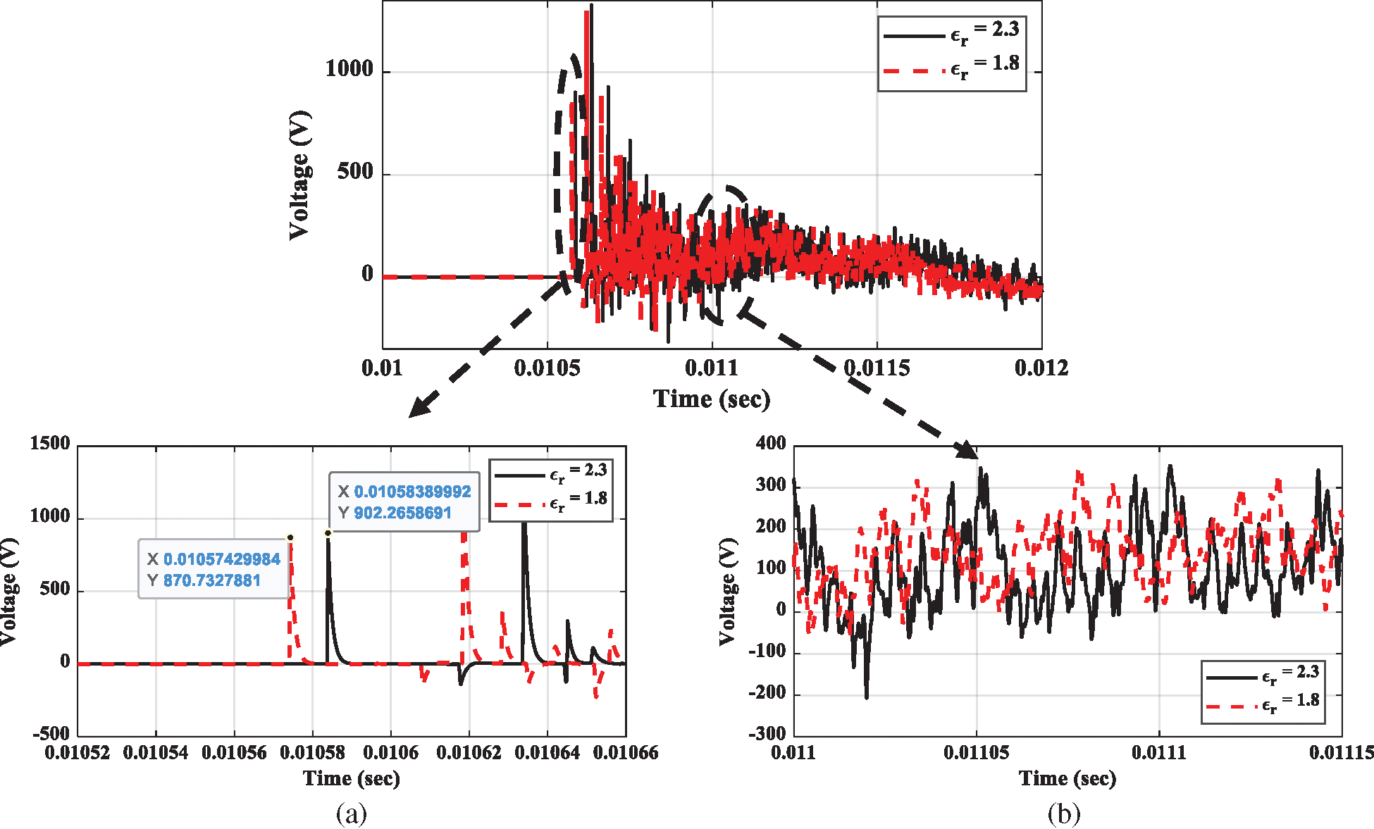
Figure 8: Load effect on the transients measured using RC transducer of unearthed networks. (a) Zooming for the first arrival surge. (b) Zooming for the reflection surges

The surge arrived at the measuring busbar at 0.01058389992 s when the relative permittivity was εr = 2.3, and arrived at 0.01057429984 s when the relative permittivity was εr = 1.8. There was an error of 0.00000960008 s (9.60008 μs) due to the permittivity change. Unfortunately, this error produces an error in the fault distance estimation: the distance error is 1536 m when the propagation speed is considered as 160 m/μs for the cable under study. Unfortunately, this distance error is high and leads to inaccurate fault location determination.

6  Effect of Load Changes on the Distribution Network Transients

The evaluation in the previous section illustrated the effect of change in relative permittivity on the transients in unearthed networks. However, that study considered only the relative permittivity recorded in the datasheet and the one for the aged cable. In this section, the effect of distributed load on the network transients due to the considered earth fault is evaluated.

6.1 Unearthed Distribution Networks

6.1.1 Fault Currents Waveforms and FFT

Fig. 9 shows the effect of load on the earth fault currents for the unearthed power distribution networks shown in Fig. 2, where the fault is at busbar E. The load conditions are as aforementioned. As shown in Fig. 9a, especially in the zoomed-in image, the effect of changing loads is low for the first 0.005 s period from the fault instant. However, an effect is observed after this period: there is shifting in the transient waveform time. At the fault instant, the dominant effect on the earth fault current transient waveforms is the fault branch itself, but after the 0.005 s period the network parameters affected the time response of the fault current waveforms as observed in the time domain performance in Fig. 9a. However, such transient time shifting is not extracted when using FFT output (as shown in Fig. 9b) because there is no time consideration. However, Fig. 9b does confirm that the load changes produce a shift in frequency and amplitude.

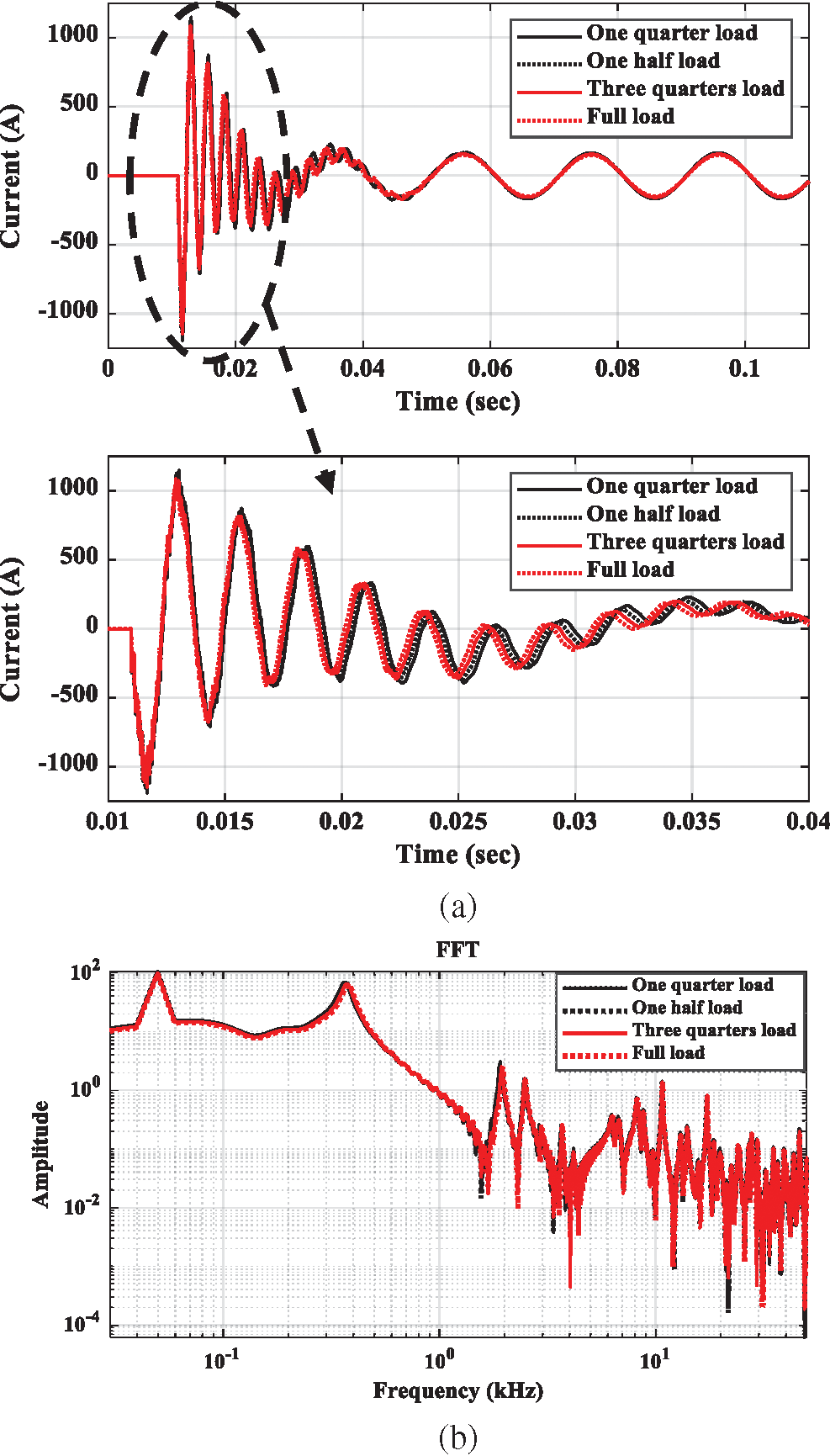
Figure 9: Load effect on the earth fault currents of unearthed networks. (a) Time domain comparison. (b) FFT-based frequency comparison

For the steady state fault period, Tab. 3 shows the earth fault current values that are changed as load changes. Since the relative permittivity is reduced at higher loading currents (see Tab. 2), the underground cable capacitances are reduced. Such capacitance reduction increases the capacitive reactance of the underground sections that reduced the earth fault currents in the unearthed networks, and vice versa.

Table 3: Fault currents (rms) in the unearthed network at different load conditions.

6.1.2 Extracted and Measured Transients Using Voltage Transducers

The evaluation in the previous subsection was at the fault point; however, the network performance evaluations are dominantly observed using the waveforms taken at the measuring point. This subsection presents the evaluation for the measurements at the main busbar A in the power distribution network shown in Fig. 2. The zoomed-in image of Fig. 10a confirms different first arrival instants with different cable parameters. Since the fault instant is 0.011 s and the arrival surge in the network with the one-quarter load condition is 0.01108289976 s, the time difference, which is measured as the time from the fault instant to the surge arrival instant at the measuring transducer, is 0.00008289976 s (82.89976 μs). The time difference is utilized for determining the fault location. Any error in this time difference produces an error in the fault location. In the zoomed-in image of Fig. 10a, the surge arrival instant is 0.01108229998 s in the network under the full load condition, and the time difference is 0.00008229998 s (82.29998 μs). From these two time differences calculated under different loads, we can see that there is an error even though the fault occurs at the same location. This error is 0.59978 μs. Taking the traveling wave speed of the cable as 160 m/μ, we can convert this error into the fault distance of 96 m. However, the network is a hybrid of overhead and underground cables. Thus, such an error can produce confusion in fault distance estimation when the traveling wave speed is 300 m/μs for the overhead lines. The zoomed-in image of Fig. 10.b shows that the measured reflected surges are completely different when different loads are considered. This is because the cable parameters change with different loads.

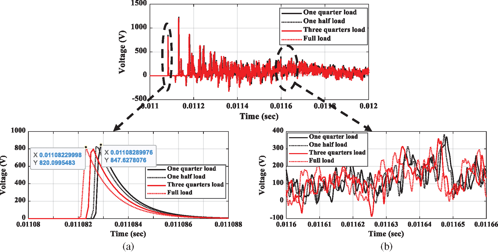
Figure 10: Load effect on the transients measured using RC transducer of unearthed networks. (a) Zooming for the first arrival surge. (b) Zooming for the reflection surges.

6.2 Compensated Distribution Networks

Fig. 11 shows the transient fault currents for different network cable capacitances when under different load conditions. As shown in Fig. 11a, the load slightly affects the currents during the first 0.005 s period from the fault instant. However, shifting in arrival instant times and peaks are observed after this 0.005 s period. Slight shifting in frequencies and amplitudes are depicted in Fig. 11b.

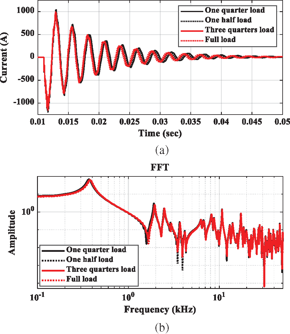
Figure 11: Load effect on the earth fault currents of compensated networks. (a) Time domain comparison. (b) FFT-based frequency comparison

Fig. 12 shows the measurements taken using the RC transducer during the earth fault event at 0.011 s for the compensated network operated at different load conditions. The zoomed-in image of Fig. 12.a confirms the changes in the first arrival surge instant. For the one quarter load condition, the surge arrives at 0.01108289976 s; by contrast, its arrival is at 0.01108229998 s for the network under the full load condition. Accordingly, the error in the first arrival surge is 0.59978 μs for the unearthed networks. The zoomed-in image of Fig. 12.b confirms that the transients due to the earth fault are affected by the load conditions.

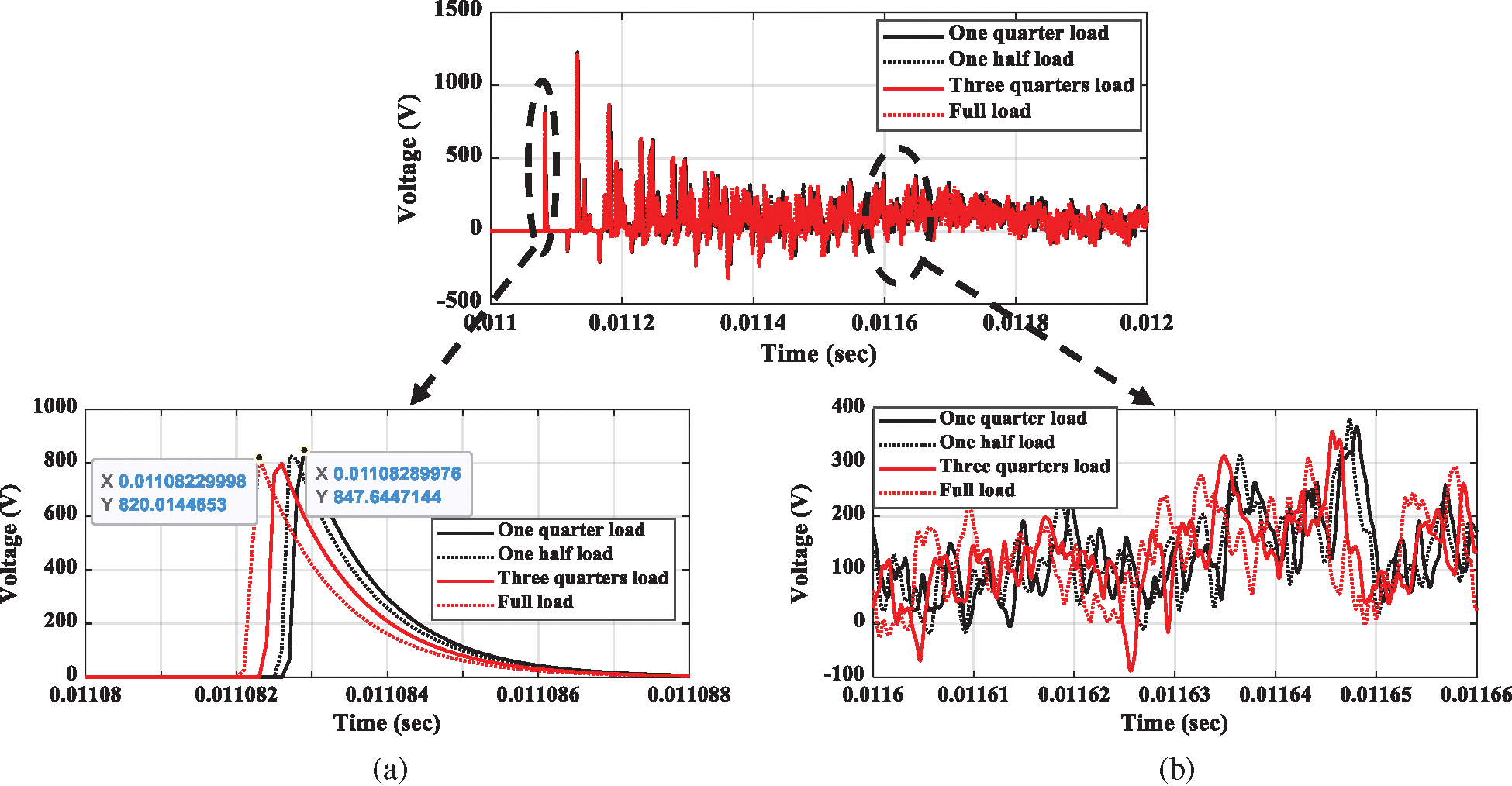
Figure 12: Load effect on the transients measured using RC transducer of compensated networks. (a) Zooming for the first arrival surge. (b) Zooming for the reflection surges

7  Conclusions

Temperature rising across XLPE of the underground cable played a very important role in the first arrival of surges under earth faults. The heat losses in the cable conductor under different load conditions were calculated using well-known equations. These calculated losses were applied to the cable conductor as a main source of heat in the simulated cable system using COMSOL Multiphysics. Temperatures of the XLPE for different cables in the utilized heterogenous unearthed/compensated distribution networks were estimated. Then, the relative permittivity of the different cable sections were evaluated based on the published experimental data. The utilized network was updated with the calculated relative permittivity values. Then, the transients due to the earth faults for both unearthed and compensated distribution networks were extracted. We conducted a frequency analysis of the transient signal and estimated the error in fault distance. With the change in relative permittivity from the datasheet value of 2.3 to the value of 1.8 (for the aged cable), there was an error of 9.60008 μs; this translated into an approximate 1536 m error in the fault distance estimation on the bases of traveling waves principles. This error was not accepted, especially for the underground cable section since where to dig and install cables must be precise. By assessing the transients under different loads, the error difference of the first arrival surge at the measuring transducer was found to be around 0.59978 μs; this represented a 96 m error in the distance estimation. Further significant differences in transients, especially after the 0.05 s period from the fault instant, were also found with load changes. This study confirms the importance of considering relative permittivity variations due to the different carrying currents for fault location algorithms. Therefore, it is recommended that fault location algorithms be able to dynamically respond to load conditions.

Acknowledgement: The authors would like to acknowledge the support from Taif University Researchers Supporting Project number (TURSP-2020/264), Taif University, Taif, Saudi Arabia.

Funding Statement: This study was funded from Taif University Researchers Supporting Project number (TURSP-2020/264), Taif University, Taif, Saudi Arabia, where the author Hend I. Alkhammash was nominated to receive the grant.

Conflicts of Interest: The authors declare that they have no conflicts of interest to report regarding the present study.

This work is licensed under a Creative Commons Attribution 4.0 International License, which permits unrestricted use, distribution, and reproduction in any medium, provided the original work is properly cited.