Intelligent Automation & Soft Computing DOI:10.32604/iasc.2021.015982
Article

Exact Analysis of Second Grade Fluid with Generalized Boundary Conditions

Syed Tauseef Saeed1,*, Muhammad Bilal Riaz2,3, Dumitru Baleanu4,5,7,*, Ali Akgül6 and Syed Muhammad Husnine1

1Department of Science & Humanities, National University of Computer and Emerging Sciences, Lahore Campus, 54000, Pakistan
2Department of Mathematics, University of Management and Technology, Lahore, 54000, Pakistan
3Institute for Groundwater Studies (IGS), University of the Free State, Bloemfontein, 9301, South Africa
4Department of Mathematics, Cankaya University, Ankara, 06790, Turkey
5Institutes of Space Sciences, Magurele, Bucharest, 077125, Romania
6Institutes of Sciences, Siirt University, Siirt, 56100, Turkey
7Department of Medical Research, China Medical University Hospital, China Medical University, Taichung, Taiwan
*Corresponding Author: Dumitru Baleanu. Email: dumitru@cankaya.edu.tr
Received: 17 December 2020; Accepted: 28 January 2021

Abstract: Convective flow is a self-sustained flow with the effect of the temperature gradient. The density is non-uniform due to the variation of temperature. The effect of the magnetic flux plays a major role in convective flow. The process of heat transfer is accompanied by mass transfer process; for instance condensation, evaporation and chemical process. Due to the applications of the heat and mass transfer combined effects in different field, the main aim of this paper is to do comprehensive analysis of heat and mass transfer of MHD unsteady second-grade fluid in the presence of time dependent generalized boundary conditions. The non-dimensional forms of the governing equations of the model are developed. These are solved by the classical integral (Laplace) transform technique/method with the convolution theorem and closed form solutions are developed for temperature, concentration and velocity. Obtained generalized results are very important due to their vast applications in the field of engineering and applied sciences. The attained results are in good agreement with the published results. Additionally, the impact of thermal radiation with the magnetic field is also analyzed. The influence of physical parameters and flow is analyzed graphically via computational software (MATHCAD-15). The velocity profile decreases by increasing the Prandtl number. The existence of a Prandtl number may reflect the control of the thickness and enlargement of the thermal effect.

Keywords: MHD second grade fluid; dynamical analysis; time dependent velocity; porous medium; Laplace transformation; radiation effect

1  Introduction

Numerous engineering practices such as drag reduction, transpiration cooling, thermal retrieval of oil, and thermite welding demand a radical knowledge of heat transfer during viscous and non-Newtonian fluids’ flow in diverse geometries. Therefore, various attempts are used to analyze and update the existing investigations corresponding to the heat transfer phenomenon. Convective flow is a self-reliant flow with the effect of the heat transfer. The influence of magnetic flux plays a significant role in convective flow. In the literature, different theories are made to see the phenomenon of heat transfer analysis. Radiation, convection and conduction are three modes of heat transfer. Convection can be defined as heat transfer by the substance motion which may be air or water. It plays a central role in creating the weather clause on the plant. Convection consists of forced and natural convection. It happens when the medium divide the heat energy and on its own move. Heat is disbursed when air is pushed by a fan, sometime heat advection referred to the forced convection. Heat is animated to distress by means of itself hotness become cause of natural convection by means of shifting source heat. In mixed convection the dualistic natures, forced and natural recurrently are transpiring collectively. When external force is applied it will also moves. This is referred as mixed convection. Heat and mass are related to each other as heat transfer rate depends on mass transfer and mass transfer further depends upon concentration difference.

Tan and Masuoka [1] have analyzed the heat transfer on Second-order fluid in the porous medium. Aldose et al. [2] have investigated the vertical plate with mixed MHD convection implanted on a porous medium. The continuity interface condition for a cylinder embedded in a porous medium has been studied by Rashidi et al. [3]. The oscillating flows of rotating Second-grade fluid has been discussed in Imran et al. [4]. Exact solutions for accelerated flows of a rotating second-grade fluid have been investigated in Khan et al. [5]. Bilal et al. [6] have analyzed the flow of Second-grade fluid generated by an accelerating flat plate. Farhad et al. [7] have discussed the closed structure for Second-grade fluid’ over a swaying vertical plate. For more details see [8–15]. Exact solutions serve in multiple ways for the specialized relevance of the streams [16–18]. Differential, rate, and integral fluids are basic categories of non-Newtonian fluid. The straight forward kind of differential fluid discussed the ordinary stresses known as the second-grade fluid. Relatively to the Newtonian fluids, a higher and complicated mathematical system exists for the non-Newtonian fluids. In 2010, Nazar et al. [19] have studied the second problem of stokes for second-grade fluids. In this model, the Laplace transform techniques helped us to acquire accurate solutions. Recently, Farhad et al. [20] have discussed the MHD fluid as electrically conducting and passing through the porous medium [21]. Researchers have discussed the different fluids on MHD free convection radiative stream over various geometries [22–30]. Ali et al. [31] have investigated the exact solution for MHD second-grade fluid in porous surfaces. The study of flow in which liquids are electrically leading within sight of attractive fields is known as MHD. The principle of the MHD is helpful for the flow against laminar to turbulence. The MHD within view of diffusion and radiation are applications of the mass and heat transfer. This paper aims to research the convection flow of the second-grade fluid using the generalized boundary condition to get a definite solution using Laplace transforms.

2  Problem Statement

Let us consider incompressible MHD second grade fluid with constant temperature saturated with porous surface lying on the plate. Suppose γ is inclination angle of the plate and magnetic field is considered as Bo with y-axis as normal to the plate. A temperature T∞′ and concentration C∞′ are at initial time τ=0. At τ>0, plate started to move with velocity w′(ζ′,τ′) having its concentration and temperature depending upon time as T∞′+Tw′l′(τ′) and C∞′+Cw′m′(τ′). The geometrical presentation of considered model is provided in Fig. 1. For such a flow, the pressure gradient is absent across the boundary layer. Under these assumptions and using Boussinesq approximation, the governing equations of the MHD Second grade fluid are given as Imran et al. [27]:

∂w′∂τ′=υ∂2w′∂ζ′2+αρ∂3w′∂τ′∂ζ′2+gβT′Cosγ−gβT∞′Cosγ+gβC′Cosγ−gβC∞′Cosγ−σB02ρw′−μk′pw′, (1)

(ρCp)∂T′∂τ′=K∂2T′∂ζ′2−∂qr∂ζ′+S(T′−T′∞), (2)

∂C′∂τ′=D∂2C′∂ζ′2+kc(C′−C′∞). (3)

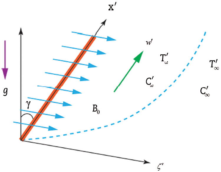
Figure 1: Geometrical presentation of second grade model

Subject to the following appropriate conditions:

τ′≤0 , w′(ζ,0)=0 , T′(ζ,0)=T∞′ , C′(ζ,0)=C∞′, ζ′≥0,

τ′>0, w′(ζ,τ)=wok′(τ′), T′(ζ,τ)=T∞′+Tw′l′(τ′), C′(ζ,τ)=C∞′+Cw′m′(τ′), ζ′=0, (4)

τ′>0 , w′(ζ,τ)→0 , T′(ζ,τ)→T∞′ , C′(ζ,τ)→C∞′, ζ′→∞.

We introduce the dimensionless variable for the simplification of governing Eqs. (1–4) of MHD second grade fluid:

ζ=w0vζ′, w=w′w0, τ=w02vτ′, T=T′−T′∞T′w, C=C′−C′∞C′w, Kr=vw02k′c, M=σBo2υρwo2,

Sc=υD, k1=υ4wo4kp, Pr=μCpK, kp=υ2wo2kp′. (5)

After substituting the dimensionless variables in Eqs. (1–4), we have dimensionless governing equations:

∂w∂τ=∂2w∂ζ2+α∂3w∂τ∂ζ2+λCosγT+NrCosγC−Mw−k1w, (6)

∂T∂τ=1Pr(1+43Rd)∂2T∂ζ2−ST, (7)

∂C∂τ=1Sc∂2C∂ζ2−KcC, (8)

with conditions:

τ≤0, w(ζ,0)=0 , T(ζ,0)=0 , C(ζ,0)=0 , ζ≥0,

τ>0, w(0,τ)=k(τ), T(0,τ)=l(τ), C(0,τ)=m(τ), ζ=0, (9)

t>0, w(ζ,τ)→0 , T(ζ,τ)→0 , C(ζ,τ)→0 , ζ→∞.

3  Solution of the Problem

3.1 Concentration Profile

Applying Laplace transformation to Eq. (8) with suitable initial condition on concentration gives:

Sc(p+Kc)=∂2C¯(ζ,p)∂ζ2. (10)

The required solution of second order differential Eq. (10) with the help of (9) on concentration is given by

C¯(ζ,p)=m(p)e−ζSc(p+Kc). (11)

Then, have

C(ζ,τ)=∫0τm′(τ−p)℘(ζSc,p,Kc,0)dp. (12)

The Sherwood number is given in Siddique et al. [28]:

Sh=−∂C∂ζ|ζ=0, (13)

Sh=ScKc∫0τm′(τ−p)erfc(Kcp)dp+Scπ∫0τm′(τ−p)pe−Kcpdp. (14)

3.2 Temperature Profile

Applying the Laplace transformation to Eq. (7) with suitable initial condition on temperature gives:

(p+S)T¯(ζ,p)=1Pr(1+43Rd)∂2T¯(ζ,p)∂ζ2. (15)

The solution of the second order differential Eq. (15) with the help of Eq. (9) on temperature is given by

T¯(ζ,p)=l(p)e−ζPrZ(p+S). (16)

Then, we obtain

T(ζ,τ)=∫0τl′(τ−p)℘(ζPrZ,p,S,0)dp. (17)

Nusselt number is given by Siddique et al. [28]:

Nu=−∂T∂ζ|ζ=0, (18)

Sh=PrZS∫0τl′(τ−p)erfc(Sp)dp+PrZπ∫0τl′(τ−p)se−Spdp. (19)

3.3 Velocity Profile

Applying the Laplace transformation to Eq. (6) with suitable initial condition on velocity yields:

(p+M+k11+αp)w¯(ζ,p)=∂2w¯(ζ,p)∂ζ2+λcos⁡γ1+αpT¯(ζ,p)+λNrcos⁡γ1+αpC¯(ζ,p). (20)

The general solution of Eq. (20) with the help of Eqs. (11) and (16) with boundary conditions on velocity is given by:

w¯(ζ,p)=k(p)e−ζp+a01+αp+λZcos⁡γl(p)2a1A(p−A1)[e−ζp+a01+αp−e−ζPr(p+S)Z]−λZcos⁡γl(p)2a1A(p+A2)[e−ζp+a01+αp−e−ζPr(p+S)Z]

+λNrcos⁡γm(p)2a3B(p−B1)[e−ζp+a01+αp−e−ζSc(p+Kc)]−λNrcos⁡γm(p)2a3B(p+B2)[e−ζp+a01+αp−e−ζSc(p+Kc)]. (21)

The above equation can be presented in suitable form as:

w¯(ζ,p)=k(p)e−ζb0p′b1+p′+λZcos⁡γl(p)2a1A(p−A1)[e−ζd0p⌢d1+p⌢−e−ζPr(p+S)Z]−λZcos⁡γl(p)2a1A(p+A2)[e−ζd0p⌢d1+p⌢−e−ζPr(p+S)Z]

+λNrcos⁡γm(p)2a3B(p−B1)[e−ζd0p⌢d1+p⌢−e−ζSc(p+Kc)]−λNrcos⁡γm(p)2a3B(p+B2)[e−ζd0p⌢d1+p⌢−e−ζSc(p+Kc)], (22)

where p⌢=p+a0,d0=1α,d1=1α−a0,a0=M+k1,a1=αPr,a2=Pr−αSPr−Z,

a3=SPr+a0Z,a4=αSc,a5=Sc+αKcSc−1,a6=a0−ScKc,Z=1+43Rd,

A=4a1a3+a224a12,A1=A−a22a1,A2=A+a22a1,B=4a4a6+a524a42,B1=B−a52a4,B2=B+a52a4.

Then, we reach

w(ζ,τ)=∫0τk′(τ−p)ℑ^1dp+λcos⁡γZ2a1A∫0τl(τ−p)(ℑ^1+ℑ^2−ℑ^3)dp−λcos⁡γZ2a1A∫0τl(τ−p)(ℑ^1+ℑ^4−ℑ^5)dp+λcos⁡γNr2a3B∫0τm(τ−p)(ℑ^1+ℑ^6−ℑ^7)dp−λcos⁡γNr2a3B∫0τm(τ−p)(ℑ^1+ℑ^8−ℑ^9)dp. (23)

The Eq. (23) is the expression for velocity with generalized boundary conditions on temperature, concentration and velocity.

3.4 Special Cases

In Eq. (22), we consider l(p)=m(p)=1p . Then, we obtain

w¯(ζ,p)=k(p)e−ζb0p′b1+p′+λZcos⁡γa3p[e−ζd0p⌢d1+p⌢−e−ζPr(p+S)Z]+λZcos⁡γl(p)A(2a1A+a2)(p−A1)[e−ζd0p⌢d1+p⌢−e−ζPr(p+S)Z]−λZcos⁡γl(p)2a1A(p+A2)[e−ζd0p⌢d1+p⌢−e−ζPr(p+S)Z]−λNrcos⁡γa6p[e−ζd0p⌢d1+p⌢−e−ζSc(p+Kc)]+λNrcos⁡γm(p)2a3B(p−B1)[e−ζd0p⌢d1+p⌢−e−ζSc(p+Kc)]−λNrcos⁡γm(p)2a3B(p+B2)[e−ζd0p⌢d1+p⌢−e−ζSc(p+Kc)]. (24)

Then, we get

w(ζ,τ)=∫0τk′(τ−p)ℑ^1dp−λZcos⁡γa3(ℑ^1−ℑ^10)+λcos⁡γZA(2a1A+a2)(ℑ^1+ℑ^2−ℑ^3)

−λcos⁡γZA(2a1A+a2)(ℑ^1+ℑ^4−ℑ^5)−λNrcos⁡γa6(ℑ^1−ℑ^11)+λcos⁡γNrB(2a4B+a5)(ℑ^1+ℑ^6−ℑ^7)

+λcos⁡γNrB(2a4B−a5)(ℑ^1+ℑ^8−ℑ^9). (25)

Consider the different cases of k(p) on velocity field using Eq. (24)

3.4.1 k(τ)=w0H(τ) (Motion of plate with constant velocity)

The solution of Eq. (24) using Heaviside unit step function can be written as:

w(ζ,τ)=ℑ^1−λZcos⁡γa3(ℑ^1−ℑ^10)+λcos⁡γZA(2a1A+a2)(ℑ^1+ℑ^2−ℑ^3)−λcos⁡γZA(2a1A+a2)(ℑ^1+ℑ^4−ℑ^5)

−λNrcos⁡γa6(ℑ^1−ℑ^11)+λcos⁡γNrB(2a4B+a5)(ℑ^1+ℑ^6−ℑ^7)+λcos⁡γNrB(2a4B−a5)(ℑ^1+ℑ^8−ℑ^9). (26)

3.4.2 k(τ)=τ (Motion of the plate with constant acceleration)

The required solution of Eq. (24) is given as:

w(ζ,τ)=∫0τℑ^1dτ−λZcos⁡γa3(ℑ^1−ℑ^10)+λcos⁡γZA(2a1A+a2)(ℑ^1+ℑ^2−ℑ^3)−λcos⁡γZA(2a1A+a2)(ℑ^1+ℑ^4−ℑ^5)

−λNrcos⁡γa6(ℑ^1−ℑ^11)+λcos⁡γNrB(2a4B+a5)(ℑ^1+ℑ^6−ℑ^7)+λcos⁡γNrB(2a4B−a5)(ℑ^1+ℑ^8−ℑ^9). (27)

3.4.3 k(τ)=eaτ (Motion of plate with exponential acceleration)

The solution of Eq. (24) using k(τ)=eaτ can be written as:

w(ζ,τ)=ℑ^1+ℑ^12−λZcos⁡γa3(ℑ^1−ℑ^10)+λcos⁡γZA(2a1A+a2)(ℑ^1+ℑ^2−ℑ^3)−λcos⁡γZA(2a1A+a2)(ℑ^1+ℑ^4−ℑ^5)

−λNrcos⁡γa6(ℑ^1−ℑ^11)+λcos⁡γNrB(2a4B+a5)(ℑ^1+ℑ^6−ℑ^7)+λcos⁡γNrB(2a4B−a5)(ℑ^1+ℑ^8−ℑ^9). (28)

3.4.4 k(τ)=cos⁡(ωτ) (Motion of plate with cosine oscillation)

The solution of Eq. (24) using k(τ)=cos⁡(ωτ) can be written as:

w(ζ,τ)=ζcos⁡(ωτ)2a0π∫0∞e−ζ24α0u−uuudu+ζb12a0π∫0τ∫0∞cos⁡(ωτ−ωp)e−ζ24α0u−u−b1pI(2b1up)dudp

−λZcos⁡γa3(ℑ^1−ℑ^10)+λcos⁡γZA(2a1A+a2)(ℑ^1+ℑ^2−ℑ^3)−λcos⁡γZA(2a1A+a2)(ℑ^1+ℑ^4−ℑ^5)

−λNrcos⁡γa6(ℑ^1−ℑ^11)+λcos⁡γNrB(2a4B+a5)(ℑ^1+ℑ^6−ℑ^7)+λcos⁡γNrB(2a4B−a5)(ℑ^1+ℑ^8−ℑ^9). (29)

Where

ℑ^1=℧(ζ,p⌢,d0,d1), ℑ^2=℘(ζ,p⌢,d0,d1,A1), ℑ^3=Ψ(ζ,p,A1,S,PrZ), ℑ^4=℘(ζ,p⌢,d0,d1,−A2), ℑ^5=Ψ(ζ,p,−A2,S,PrZ), ℑ^6=℘(ζ,p⌢,d0,d1,B1), ℑ^7=Ψ(ζ,p,B1,Kc,Sc), ℑ^8=℘(ζ,p⌢,d0,d1,−B2), ℑ^9=Ψ(ζ,p,−B2,Kc,Sc), ℑ^10=℘(ζPrZ,p,S,0), ℑ^11=℘(ζSc,p,Kc,0), ℑ^12=℘(ζ,p⌢,d0,d1,a),

Eq. (29) explores the required exact solutions of the second grade fluid for the cosine and sine oscillation respectively.

3.5 Validation of Results

•    In this case, if second grade parameter α=0 and radiation Rd=0 we get the similar solutions obtained by Imran et al. (Eq. (32) in Imran et al. [27]). These results show the validation of our general results.

•    In the void of magnetic field B0=0 , concentration C=0 and S=0 , the governing equations reduce to Farhad et al. [7]. The condition on temperature l(τ)=1 and w(ζ,τ)=H(τ)cos⁡(ωτ)/H(τ)sin⁡(ωτ) , we get the same result as shown in Farhad et al. (Eqs. (22)–(28) in Farhad et al. [7]). These solutions are identical to our general results.

•    If we neglect the effect of temperature T=0 , magnetic field B0=0 and concentration C=0 then the required results are identical by Nazar et al. (Eqs. (14)–(19) in Nazar et al. [19]).

4  Results and Discussion

In this paper, we investigated the unsteady uniform free convection flow (stream) of the second-grade fluid passing through an accelerated limitless plate with constant temperature inserted in the permeable medium. Analytical solutions can be achieved through the Laplace transform method. The graphical representation helps us to show the influences of different physical parameters such as Rd, M, Pr, Sc, Kc, angle of inclination γ and second grade parameter α on velocity. Fig. 2 analyzes the variation of Rd, on the velocity with help of time. The large value of radiation parameter Rd, causes to increase in the fluid flow. The rate of energy transports of fluid increase due to an increase in the intensity of the radiation parameter and decrease the viscosity. Due to such behavior fluid moves faster and enhances the fluid velocities. Fig. 3 shows the influence of magnetic field on velocity components. This graphical representation indicates that an increase in the magnetic field, the velocity reduce due to Lorentz force. It behaves as a drag force. By increasing the parameter of the magnetic field, the Lorentz force also increases. Fluid flow on the boundary layer is slow down due to this force. Fig. 4 shows the behavior of Prandtl number. Specific heat and conductivity depend on Pr. It is the ratio of kinematic viscosity and thermal diffusivity. The thickness of the momentum and boundary layer is control by the Prandtl number. It is seen from the graph, decreasing the velocity, observed by increase the value of Pr . The lower Prandtl number enhances thermal conductivity and increase the boundary layer. The permeability parameter of porous medium k1 increase the velocities because the large value of k1 reduce the resistance and increase the momentum which accelerates the fluid motion. The behavior of k1 is shown in Fig. 5. Fig. 6 analyzes the behavior of the second-grade fluid parameter α . The behavior clearly shows that the large values of α have greater stability as compared to a lower value. Fig. 7 shows the impact on Schmidt number for velocity field versus time. It is defined as the ratio between the viscous diffusion rate and mass diffusion rate. Physically, Schmidt number is used to characterize fluid motion and it relates the thickness of hydro-dynamic layers and mass transfer boundary layers. The velocity and concentration boundary layers in Schmidt number almost coincide with each other, because diffusion of mass and momentum are comparable. It is observed that by the larger value of Sc , the velocity becomes decreases. The effect of boundary layer thickness is discussed by changing the inclination angle γ on fluid velocity in Fig. 8. It shows that with increasing the value of γ , the velocity and boundary layer thickness becomes decrease when fluid is moving. As increases in time, the less value of the inclination angle has larger velocity. Fig. 9 shows the impact of Kc on the velocity profile. It is noted that velocity increase as an increase of Kc .

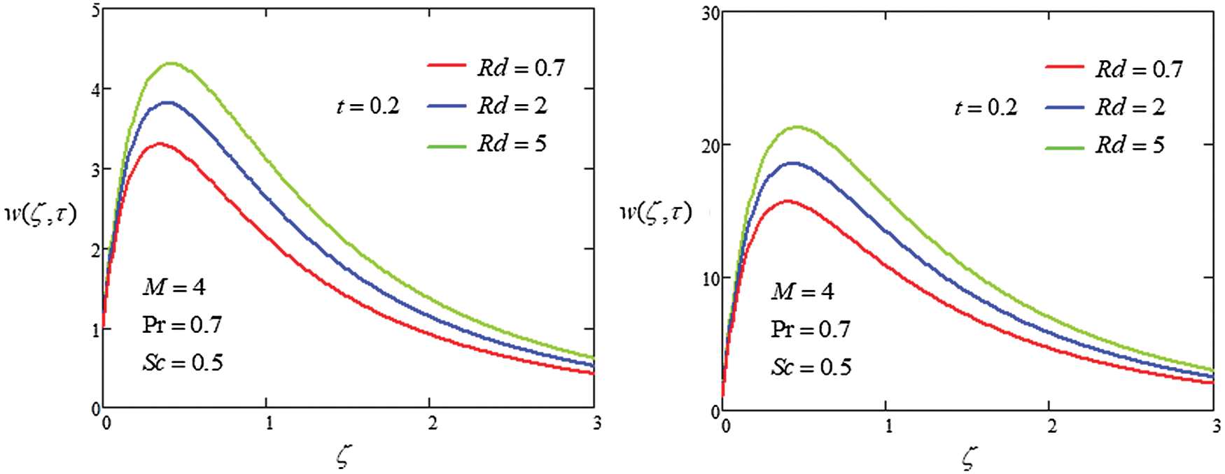
Figure 2: Plot velocity profile with different values of Rd

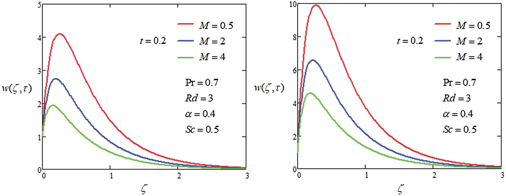
Figure 3: Plot velocity profile with different values of M

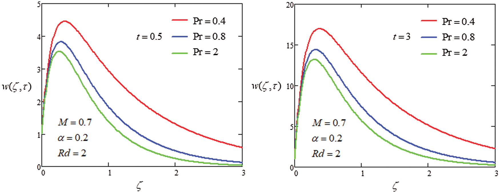
Figure 4: Plot velocity profile with different values of Pr

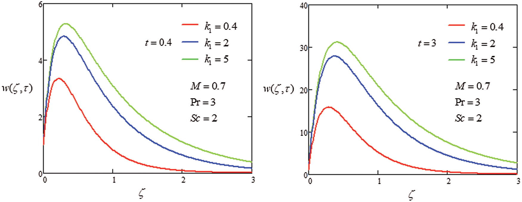
Figure 5: Plot velocity profile with different values of k1

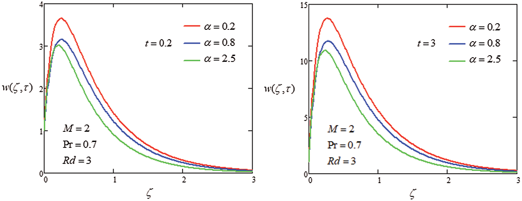
Figure 6: Plot velocity profile with different values of α

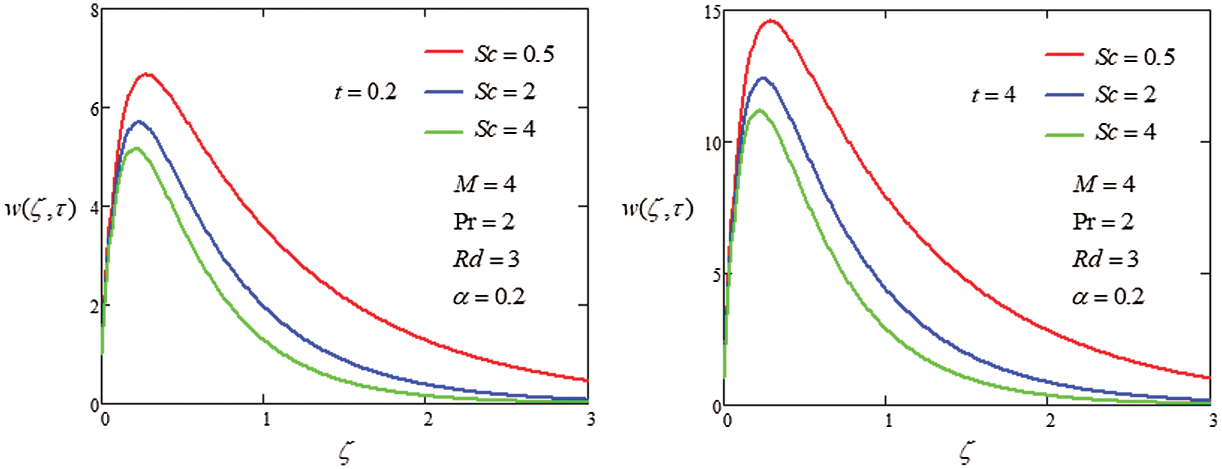
Figure 7: Plot velocity profile with different values of Sc

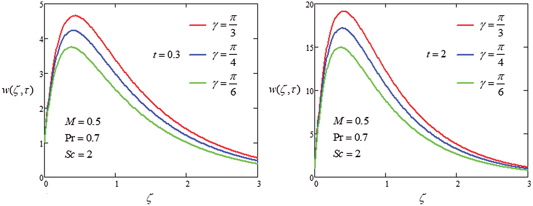
Figure 8: Plot velocity profile with different values of γ

Figure 9: Plot velocity profile with different values of Kc

5  Conclusion

The analysis of heat transfer on the MHD flow of generalized second grade in porous medium was investigated through Laplace transformation to get the closed form solutions. The graphical approach was used to discuss the influence of parameter on velocity. The following points were extracted from the instant study

     i)  Increasing the value of α , Pr and M decrease fluid velocity.

    ii)  Increase velocity field when γ decrease.

   iii)  Enhance the fluid motion by existence of free convection.

    iv)  Velocity increase as an increase of Kc .

Acknowledgement: The authors are highly thankful and grateful for support of this research article.

Funding Statement: The authors received no specific funding for this study.

Conflicts of Interest: The authors declare that they have no conflicts of interest to report regarding the present study.

References

 1.  W. Tan and T. Masuoka. (2005). “Stoke’s first problem for a second grade fluid in a porous half-space with heated boundary,” International Journal of nonLinear Mechanics, vol. 40, no. 4, pp. 515–522. [Google Scholar]

 2.  T. K. Aldoss, M. A. Al-Nimr, M. A. Jarrah and B. Al-Shaer. (1995). “Magnetohydrodynamics mixed convection from a vertical plate embedded in a porous medium,” Numerical Transfer Heat Application, vol. 28, no. 5, pp. 635–645. [Google Scholar]

 3.  S. Rashidi, A. Nouri-Borujerdi, M. S. Valipour, R. Ellahi and I. Pop. (2015). “Stress-jump and continuity interface conditions for a cylinder embedded in porous medium,” Transport porous Media, vol. 107, no. 1, pp. 171–186. [Google Scholar]

 4.  M. A. Imran, M. M.Imran and C. Fetecau. (2014). “MHD oscillating flows of rotating second grade fluid in a porous medium,” Communications in Nonlinear Science and Numerical Simulation, Vol. 2014, pp. 1–12. [Google Scholar]

 5.  I. Khan, A. Farhad and M. Norzieha. (2010). “Exact solutions for accelerated flows of a rotating second grade fluid in a porous medium,” World Applied Sciences Journal, vol. 9, pp. 55–68. [Google Scholar]

 6.  M. B. Riaz, A. A. Zafar and D. Vieru. (2015). “On flows of generalized second grade fluids generated by an oscillating flat plate, MATEMATICĂ,” MECANICĂ TEORETICĂ. FIZICĂ, vol. 1, pp. 1–9. [Google Scholar]

 7.  F. Ali, I. Khan and S. Shafie. (2014). “Closed form solutions for unsteady free convection flow of a second grade fluid over an oscillating vertical plate,” PLoS One, vol. 9, no. 2, pp. 1–15. [Google Scholar]

 8.  M. Hussain, T. Hayat, S. Asghar and C. Fetecau. (2010). “Oscillatory flows of second grade fluid in a porous space,” Nonlinear Analysis & Real World Application, vol. 11, pp. 2403–2414. [Google Scholar]

 9.  M. E. Erdoğan and C. E. İmrak. (2005). “An exact solution of the governing equation of a fluid of second grade for three dimensional vortex flow,” International Journal of Engineering Science, vol. 43, no. 15–16, pp. 721–729. [Google Scholar]

10. C. Fetecau and C. Fetecau. (2005). “Starting solutions for some unsteady unidirectional flow of a second grade fluid,” International Journal of Engineering Science, vol. 43, pp. 781–789. [Google Scholar]

11. S. Asghar, S. Nadeem, K. Hanif and T. Hayat. (2006). “Analytic solution of Stokes’ second problem for second gradefluid,” Mathematical Problems in Engineering, vol. 2006, pp. 1–9. [Google Scholar]

12. A. K. Tiwari and S. K. Ravi. (2009). “Analytical studies on transient rotating flow of a second grade fluid in a porous medium,” Advances in Theoretical and Applied Mechanics, vol. 2, pp. 33–41. [Google Scholar]

13. C. Fetecau and C. Fetecau. (2005). “Starting solutions for the motion of second grade fluid,” International Journal of Engineering Science, vol. 43, pp. 781–789. [Google Scholar]

14. I. Khan, R. Ellahi and C. Fetecau. (2008). “Some MHD flows of second grade fluid through the porous medium,” Journal of Porous Media, vol. 11, pp. 389–400. [Google Scholar]

15. C. Fetecau and C. Fetecau. (2006). “Starting solutions for the motion of a second grade fluid due to longitudinal and torsional oscillations of a circular cylinder,” International Journal of Engineering Science, vol. 44, no. 11–12, pp. 788–796. [Google Scholar]

16. S. H. Hsu and A. M. Jamieson. (1993). “Viscoelastic behavior at the thermal sol-gel transition of gelatin,” Polymer, vol. 34, pp. 2602–2608. [Google Scholar]

17. R. Bandelli. (1995). “Unsteady unidirectional flows of second grade fluids in domains with heated boundaries,” International Journal of NonLinear Mechanics, vol. 30, pp. 263–269. [Google Scholar]

18. R. A. Damesh, A. S. Shatnawi, A. J. Chamkha and H. M. Duwairi. (2008). “Transient mixed convection flow of second grade viscoelastic fluid over a vertical surface,” Nonlinear Analysis: Modelling and Control, vol. 13, no. 2, pp. 169– 179. [Google Scholar]

19. M. Nazar, C. Fetecau, D. Vieru and C. Fetecau. (2010). “New exact solutions corresponding to the second problem of stokes for second grade fluids,” Nonlinear Analysis: Real World Application, vol. 11, pp. 584–591. [Google Scholar]

20. F. Ali, M. Norzieha, S. Sharidan, I. Khan and T. Hayat. (2012). “New exact solutions of stokes second problem for an MHD second grade fluid in a porous space,” International Journal of Nonlinear Mechanics, vol. 47, pp. 521–525. [Google Scholar]

21. O. D. Makinde, W. A. Khan and J. R. Culham. (2016). “MHD variable viscosity reacting flow over a convectively heated plate in a porous medium with thermophoresis and radiative heat transfer,” International Journal of Heat & Mass Transfer, vol. 93, pp. 595–604. [Google Scholar]

22. M. Sheikholeslami, D. D. Ganji, M. Y. Javed and R. Ellahi. (2015). “Effect of thermal radiation on MHD nanofluid flow and heat transfer by means of two phase model,” Journal of Magnetism and Magnetic Materials, vol. 374, no. 1, pp. 36–43. [Google Scholar]

23. C. Zhang, L. Zheng, X. Zhang and G. Chen. (2015). “MHD flow and radiation heat transfer of nanofluid in porous media with variable surface heat flux and chemical reaction,” Applied Mathematical Modeling, vol. 39, no. 1, pp. 165–181. [Google Scholar]

24. M. M. Rashidi, M. Ali, N. Freidoonimehr, B. Rostami and M. A. Hossain. (2014). “Mixed convective heat transfer for MHD viscoelastic fluid flow over a porous wedge with thermal radiation,” Advance Mechanical Engineering, vol. 6, pp. 735939. [Google Scholar]

25. M. Dehghan, Y. Rahmani, D. D. Ganji, S. Saedodin, M. S. Valipour et al. (2015). , “Convection–radiation heat transfer in solar heat exchangers filled with a porous medium: Homotopy perturbation method versus numerical analysis,” Renewable Energy, vol. 74, no. 1, pp. 448–455. [Google Scholar]

26. P. Chandrakala and P. N. Bhaskar. (2009). “Thermal radiation effects on MHD flow past a vertical oscillating plate,” International Journal of Applied Mechanical Engineering, vol. 14, pp. 349–358. [Google Scholar]

27. M. A. Imran, A. Maryam, M. B. Raiz, R. Ali and I. Khan. (2019). “A comprehensive report on convective flow of fractional (ABC) and (CF) MHD viscous fluid subject to generalized boundary conditions,” Chaos, Solitons & Fractals, vol. 118, no. 10, pp. 274–289. [Google Scholar]

28. I. Siddique, I. Tlili, M. Bukhari and Y. Mahsud. (2020). “Heat transfer analysis in convective flows of fractional second grade fluids with Caputo-Fabrizio and Atangana-Baleanu derivative subject to Newtonian heating,” Mechanics of Time-Dependent Materials, vol. 9, no. 2, pp. 1. [Google Scholar]

29. T. Anwar, P. Kumam, Asifa, I. Khan and P. Thounthong. (2020). “An exact analysis of radiative heat transfer and unsteady MHD convective flow of a second grade fluid with ramped wall motion and temperature,” Heat Transfer, vol. 50, no. 1, pp. 196–219. [Google Scholar]

30. S. Kirtphaiboon, U. Humphries, A. Khan and A. Yusuf. (2021). “Model of rice blast disease under tropical climate conditions,” Chaos, Solitons & Fractals, vol. 143, no. 8, pp. 110530. [Google Scholar]

31. F. Ali, M. Norzieha, S. Sharidan, I. Khan and T. Hayat. (2012). “New exact solutions of Stokes second problem for an MHD second grade fluid in a porous space,” International Journal of Non-Linear Mechanics, vol. 47, no. 5, pp. 521–525. [Google Scholar]

Appendix A.

Ψ(ς,t,a,b,c)=eat2(e−ζcs+berfc(ζc2t−at+bt)+eζcs+berfc(ζc2t+at+bt)) (A1)

L−1(℧(ζ,s,a,b))=1−2aπ∫0∞sin⁡(ζx)x(a+x2)exp⁡(−btx2a+x2)dx (A2)

L−1(℘(ζ,s,a,b,c))=exp⁡(ct−ζacb+c)−1−2acπ∫0∞sin⁡(ζx)x(ac+bx2+cx2)exp⁡(−btx2a+x2)dx (A3)

This work is licensed under a Creative Commons Attribution 4.0 International License, which permits unrestricted use, distribution, and reproduction in any medium, provided the original work is properly cited.