DOI:10.32604/iasc.2021.010131
| Intelligent Automation & Soft Computing DOI:10.32604/iasc.2021.010131 | |
| Article |
Soil Moisture Prediction in Peri-urban Beijing, China: Gene Expression Programming Algorithm
1Liaoning Vocational College of Ecological Engineering, Shenyang, 110122, China
2National Engineering Research Center for Information Technology in Agriculture, Beijing Academy of Agriculture and Forestry Sciences, Beijing 100097, China
3Beijing Agricultural Technology Extension Station, Beijing, 100029, China
4Yunnan Agricultural Vocational and Technical College, Kunming, 650031, China
5Key Laboratory for Quality Testing of Hardware and Software Products on Agricultural Information, Ministry of Agriculture, Beijing, 100097, China
*Corresponding Author: Xin Zhang. Email: zhangx@nercit.org.cn
Received: 30 August 2020; Accepted: 02 October 2020
Abstract: Soil moisture is an important indicator for agricultural planting and agricultural water management. People have been trying to guide crop cultivation, formulate irrigation systems, and develop intelligent agriculture by knowing exactly what the soil moisture is in real time. This paper considers the impact of meteorological parameters on soil-moisture change and proposes a soil-moisture prediction method based on the Gene Expression Programming (GEP) algorithm. The prediction model is tested on datasets from Shunyi, Yanqing and Daxing agricultural farms, Beijing. The results show that the GEP model can predict soil moisture with a maximum correlation coefficient of 0.98, and the root-mean-square errors in three different farms were below 2.32.
Keywords: GEP; prediction; soil moisture
Soil moisture is an important factor related to the crop growth environment, which directly affects crop growth and fruit quality. With the development of society and the growth of the population, the global water shortage problem is becoming more and more serious. This requires all trades and professions to save water while they are developing. In view of agricultural water, we should strive to maximize the benefits of limited water and achieve a precise understanding of agricultural water. This requires us to be able to accurately grasp the soil-moisture content in real time and predict the change in soil moisture over a certain period of time in the future.
As early as the 20th century, the prediction of soil moisture began. It can be roughly divided into the empirical formula method [1], the water balance method, the regression index method [2], the soil dynamics method, the time series method [3], the neural network method [4–7], and the remote sensing monitoring method. The empirical formula method and water balance method always need certain parameters which are important to the results but difficult to correct. In recent years, with the deepening of the research of brain science and the deepening of the understanding of the operation of the brain, neural networks, and the internal processing mechanisms of nerve cells, the neural network was developed on the basis of simulating a human brain’s thought activities. This has developed vigorously in recent years [8–12]. Camacho Poyato et al. proposed a new method for the short-term prediction of daily irrigation water demand under the condition of limited data validity. This method combines the structure of (Artificial Neural Network) ANN, a Bayesian framework, and a genetic algorithm (GA) and achieved ideal results in an irrigation district in southern Spain. Huang et al. [13] established the (Back Propagation) BP model to predict the soil-moisture content of Hongxing Farm in Heilongjiang Province. Lingmiao Huang established a simplified BP soil-moisture prediction model based on default factors. Some other neural networks, such as the dynamic neural network and the (Radical Basis Function) RBF neural network and so on [14–16], were gradually used to predict soil moisture. With the development of different models in soil-moisture content prediction, the applicability and accuracy of the situation deserves to be further evaluated. Abhishek Pandey et al. from India used microwave data and the artificial neural network algorithm to predict soil-moisture content. The artificial neural network was trained by transmitting and receiving microwave data under different soil conditions through an X-band microwave scatterer. Then, the trained neural network was used to predict soil moisture. Affected by soil characteristics, meteorology, and crop and agricultural operations, the prediction of agricultural soil moisture is a great challenge [17]. With the development of precision agriculture, there are higher requirements for the accurate prediction of soil moisture. However, traditional neural networks run slowly and are prone to over-fitting according to Quadri et al. [18] and Tiwari et al. [19].
Gene Expression Programming (GEP) was proposed by a Portuguese scholar named Ferreira. At that time, genetic algorithm (GA) and genetic programming (GP) were mature. Ferreira integrated the advantages of GA and GP and integrated the simple and fast features of GA’s fixed-length linear coding. In gene expression (semantic expression), GEP uses simple coding to solve complex problems by inheriting the flexible tree structure of GP. In addition, genetic manipulation causes most chromosome death by inserting, deleting, crossing, and mutating genes, while GEP introduces very loose head and tail constraints. It has been proved that all chromosomes satisfying head and tail constraints survive under genetic manipulation, which makes GEP 2–4 orders of magnitude faster than GA and GP.
The emergence of gene expression provides people with a new means of prediction [20]. For example, S. Emamgolizadeh et al. [21] predicted the cation exchange capacity of soil based on two farms in Iran, which showed that it was feasible and accurate to predict the cation exchange capacity of soil using gene expression. Razaq et al. [22] used gene expression to predict the flow time curve on the eastern coast of the Malaysia Peninsula. The results show that the prediction accuracy of gene expression is very high. Nematzadeh et al. [23] investigated the compressive performance of fiber-reinforced concrete containing recycled PET chips being exposed to high temperatures in their experimental effort. In addition, they developed a closed-form formula to predict the compressive strength using the gene expression programming (GEP) approach. The results showed that the model worked well. Wang Sheng et al. simulated the monthly reference crop evapotranspiration in Hunan and Hubei based on GEP, and determined its feasibility in crop evapotranspiration prediction. On the basis of the superiority of the GEP algorithm, this paper integrates the five-year long series of data from the Beijing area in order to: (1) establish a GEP algorithm model suitable for soil-moisture prediction; (2) validate the applicability of the GEP algorithm to farms in different geomorphic regions of Beijing area [24,25].
The data used in this study were provided by the Beijing Meteorological Service, including meteorological data and soil-moisture data. In the series of 2012–2016, the soil-moisture data is the soil volume moisture content at 0 cm–20 cm depth, which is per unit, and the meteorological data include temperature, air pressure, humidity, wind speed, ground temperature, rainfall, and initial moisture value. After preliminary integration, Shunyi Farm (46°6′N,116°52′E) has 1147 datasets, Yanqing Farm (40°27′N,115°46′E) has 1123 datasets. and Daxing Farm (39°43′N,116°21′E) has 1213 datasets.
The building and training of the model required a large amount of data, so 992 sets of Shunyi data from 2012 to 2015, 968 sets of Yanqing data, and 959 sets of Daxing data were used for this work.
The operation of the GEP model can be divided into five steps:
(1) The first step is to select the fitness function. All evolutionary algorithms need to evaluate the environmental adaptability of newly generated chromosomes, which represent the solution of the problem. Fitness is an index to measure the environmental adaptability of species. The selection Eq. (1) is used as the final fitness function.
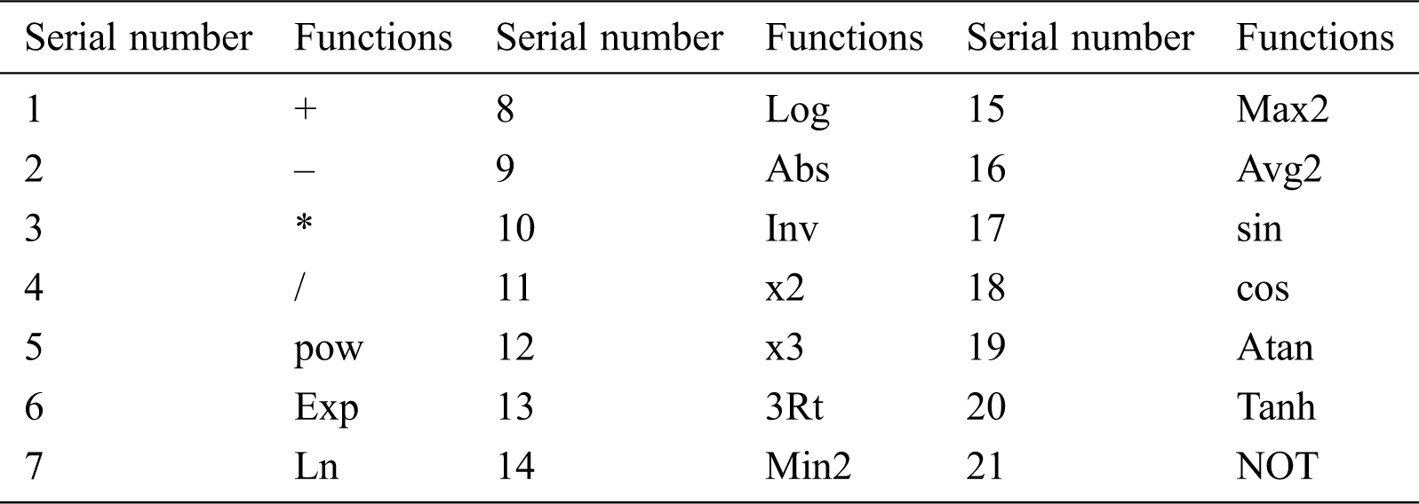
(2) The second step is to select the set of functions and the set of terminators. GEP takes two types of symbols as its components, one is the terminator set, the other is the function set, in which the terminator set is a constant or function without parameters. The set of function operators is more complex, including simple mathematical operators, Boolean operations, elementary functions, relational operations, conditional operations, and program composition in programming languages.
There are no existing rules for the selection of function sets. The selection of function sets in this paper is mainly related to three aspects. First, common sense and the most common four operations should be taken into account. Secondly, according to the literature referring to the relationship between soil moisture and climate, pow, Exp, Ln, x2, x3, log, and so on are selected. Thirdly, on the basis of the periodicity, extreme value limitation, and fluctuation of soil moisture, triangular functions with periodicity and upper and lower limits, and maximum and minimum equivalent functions are selected. The set of functions that ultimately determines the model is shown in Tab. 1.
Table 1: Functions of Gene Expression Programming (GEP) model
(3) The third step is to set the length of the head of the chromosome and the number of genes. GEP is encoded by linear symbols, which are of specified length and consist of a head and tail. Let the head length be “h” and the tail length be “e”. The maximum number of operations of all functions in the set of functions contained in the gene is “n”. The value of “E” can be calculated from the following formula:
Thus, one or more genes of equal length, linked together by connecting symbols, constitute the chromosomes of GEP. Each gene fragment in a chromosome can be decoded into a Sub-Expression Tree (Sub-ET), and multiple sub-expression trees form a more complex multi-sub-tree expression tree.
In this model, the number of chromosomes is 30, the length of gene head is 8, and each chromosome contains five genes.
(4) The fourth step is to select the join function of the subtree, and the connection between sub-trees is additive. Taking the 1D prediction period of Shunyi Farm as an example, the final chromosome expression tree of the model is shown in Fig. 1:
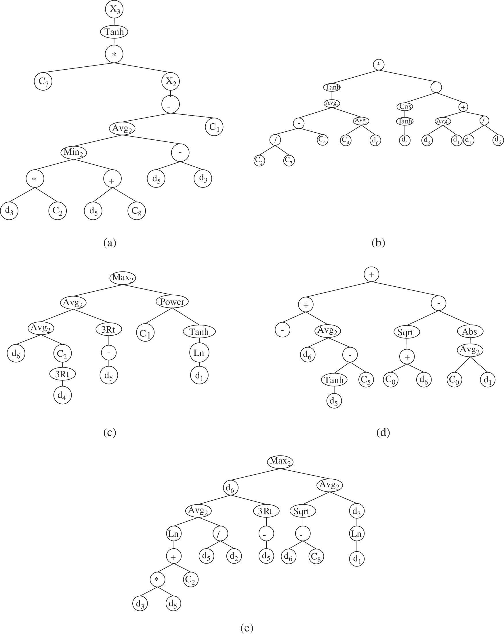
Figure 1: Polygenic chromosome expression tree. (a) Sub-Expression Tree (Sub-ET) 1 (b) Sub-ET 2 (c) Sub-ET 3 (d) Sub-ET 4 (e) Sub-ET 5
(5) The fifth step is to select the required genetic operators. The basic genetic operators of GEP are Selection, Mutation, Inversion, Insertion sequence transposition, Root insertion sequence transposition, Gene transformation, One-point recombination, Two-points recombination, and Gene recombination.
The meaning of selection is to select the paternal individuals according to their fitness for other genetic operations or evolutionary development.
Variation refers to the random testing of each chromosome on a single chromosome. When the mutation probability is satisfied, the coding of the site will be reproduced. The specific form is shown in Fig. 2.

Figure 2: Variation process
Inversion refers to the head of a gene acting on a chromosome. A substring is randomly selected in the head of a gene, and then the middle character of the substring is used as the center of symmetry to coordinate the positions of each character. The specific variation is shown in Fig. 3.

Figure 3: Inversion process
Insertion sequence transposition is a unique genetic operator of GEP. A substring is randomly selected from a gene and inserted into a randomly designated position of the head (except the first position). The other symbols of the head are extended backwards and truncated beyond the coding of the head, as shown in Fig. 4.

Figure 4: Insertion sequence transposition process
Unlike Insertion sequence transposition, the Root insertion sequence transposition specially inserts the selected substrings into the first position. The transformation process is shown in Fig. 5.

Figure 5: Root insertion sequence transposition process
Gene transformation, which is essentially a special case of IS insertion, is the element transformation between the whole gene and the starting position of chromosome.
One-point recombination refers to the random selection of a crossing position on the chromosomes of two parents, and the exchange of the chromosome parts behind the crossing points to obtain the chromosomes of two offspring shown in Fig. 6.

Figure 6: One-point recombination process
Two-points recombination also acts on two paternal chromosomes, randomly selecting two intersections on the chromosome, and then exchanging the chromosome parts between the intersections shown in Fig. 7.
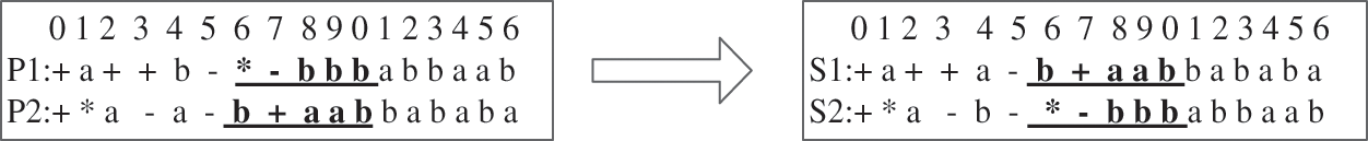
Figure 7: Two-points recombination process
Gene recombination, which occurs only on polygenic chromosomes, randomly selects one gene, and then exchanges the genes that the two paternal chromosomes want to correspond to.
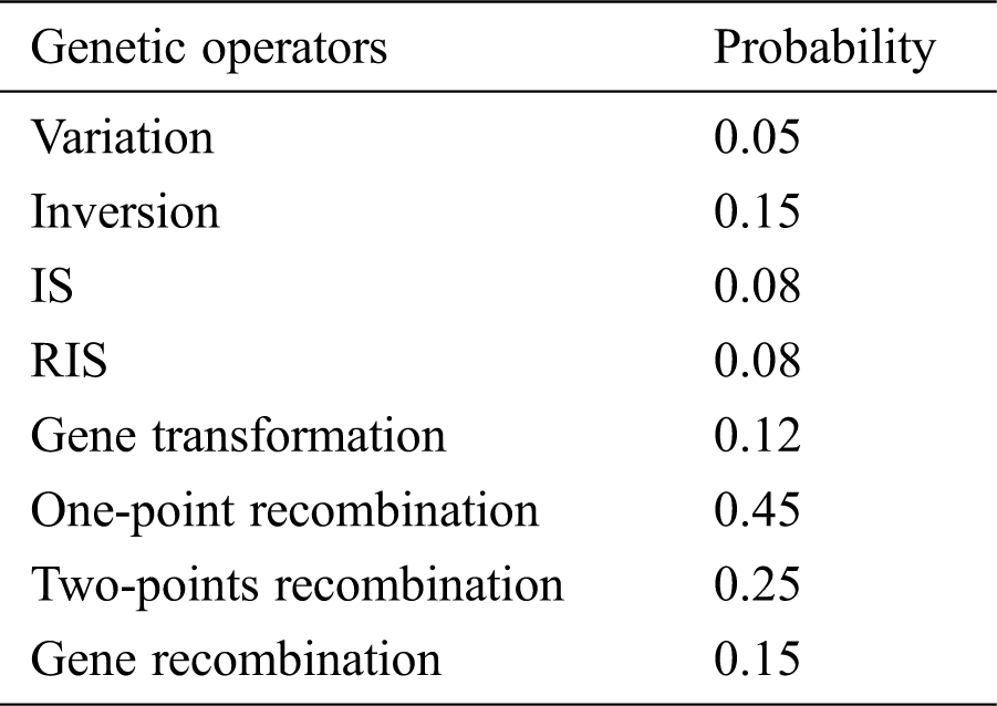
The selection and specific settings of genetic operators are shown in Tab. 2.
Table 2: Values of genetic operators employed in the GEP model
Four indicators: correlation coefficient (R2), root-mean-square error (RMSE), mean relative error (MRE), and mean absolute error (MAE), were used to evaluate the model. The calculation formulas of each evaluation index are as follows:
Correlation coefficient (R2):
Root-mean-square error (RMSE):
Mean relative error (MRE):
Mean absolute error (MAE):
where N is the number of measured data points, Oi is measured data, Pi is the Simulation results, Oavg is the average of the measured values, and Pavg is the average of simulated values.
The model was applied to Shunyi Farm, Yanqing Farm, and Daxing Farm for the practical test. In the data of 2016, there were 254 groups of Shunyi data, 254 groups of Yanqing data, and 253 groups of Daxing data. In this part of the data, 50 groups of data were randomly selected from each region as the test data of the model. The error of the model and the correlation between the predicted value and the measured value are compared.
3.1 Application in Shunyi Farm
The prediction results of soil moisture in Shunyi farm are shown in Fig. 8. It can be seen that the value of soil moisture fluctuates greatly, varying between 12% and 26%. When the prediction period is 1 day, the probability of coincidence between the predicted points and the observed points is large; When the prediction period is extended to 3 days, there is a slight difference between the prediction results and the observed values in the extreme region. When the prediction period is 5 days, the trend of prediction of soil-water content is consistent, but there is a certain deviation in the numerical value.
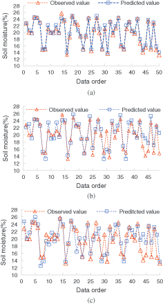
Figure 8: The prediction values of soil moisture in Shunyi (a) Prediction values in 1 day (b) Prediction values in 3 days (c) Prediction values in 5 days
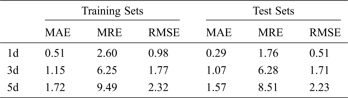
The operation error of the model is listed in Tab. 3. For the prediction of the 1-day period, the average absolute error of model training is less than 0.5%, and the root-mean-square error is 0.99, so the model is relatively stable; for the test prediction, the absolute error is only 0.29%, and the root-mean-square error is only 0.51. When the prediction period is extended to 3 days, the average relative error and the average absolute error of the model increase by about 4.52% and 0.78%, respectively, while the root-mean-square errors representing the prediction stability of the model increase by 0.79 and 1.2, respectively. When the prediction period reaches 5 days, the error of the model further increases, the absolute error increases by about 1.28% compared with the 1-day prediction period, the relative error increases by about 6.75%, and the corresponding root-mean-square errors reach 2.32 and 2.23, respectively, which shows that the prediction stability of the model is also affected by the extension of the prediction period.
Table 3: Correlation coefficient of model testing in Shunyi
3.2 Application in Yanqing Farm
According to the actual prediction results of Yanqing farm, as shown in Fig. 9, 50 groups of data were randomly selected, and the soil moisture fluctuates between 12% and 26%. When the prediction period is 1 day, the overall prediction of the model is more accurate, and the error is smaller than for the observation data; when the prediction period is extended to 3 days, the prediction volatility of the model becomes larger, and the error in the lower and higher values of soil moisture is more obvious than in other places; when the prediction period is 5 days, the trend of the model prediction data and the observation data is basically the same, but overall, some errors can be seen.
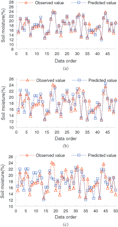
Figure 9: The prediction values of soil moisture in Yanqing (a) Prediction values in 1 day (b) Prediction values in 3 days (c) Prediction values in 5 days
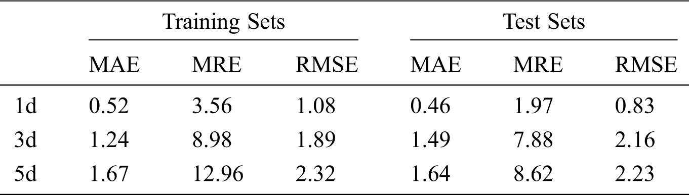
The operation error of the model in Yanqing farm is listed in Tab. 4. Compared with Shunyi, the error of the model increases and the stability of the prediction decreases. The best prediction performance occurs in the 1-day prediction period, and the corresponding average absolute error and military tracking error are 0.46% and 0.83%, respectively. When the prediction period is 3 days, the increase range of model error is smaller than that of Shunyi. The training average relative error and average absolute error increase by 0.72% and 5.42%, respectively, compared with the prediction period of 1 day, and the test average relative error and absolute error increase by 1.03% and 5.91%, respectively. When the prediction period is 5 days, the maximum average relative error of the model is 12.96%. However, the corresponding root-mean-square errors are 2.32 and 2.23, respectively.
Table 4: Correlation coefficient of model testing
3.3 Application in Daxing Farm
According to the actual prediction results of Daxing farm, as shown in Fig. 10, the soil moisture fluctuates between 12% and 28%. When the prediction period is 1 day, the fitting degree of the model simulation value and the observation value is high; when the prediction period is extended to 3 days, the soil-moisture value is high and low, the fitting is good, but when the value changes greatly, the prediction of the model slightly deviates; when the prediction period is 5 days, the trend of the prediction value and the observation value is the same, but when the soil moisture is low, a certain deviation appears, which is not even.
From the error point of view, when the best running time of the model is 1 day, the average absolute errors of the training set and the test set are 0.45% and 0.42%, the relative errors are 1.88% and 1.85%, and the root-mean-square errors are only 1.05 and 1.15, respectively. When the prediction period is 5 days, the average absolute errors of training set and test set increase by 1.26% and 1.20%, the average relative errors reach 9.88% and 8.61%, and the root-mean-square errors reach 2.29 and 2.09, respectively. When the prediction period is 3 days, the performance of the model is between the two. The average absolute error of the training set and the test set is 1.19%, the average relative errors are 7.21% and 6.43%, and the root-mean-square error is 1.89.
4 Model Comprehensive Evaluation
The correlation coefficients of the model test are shown in Fig. 11 and Tab. 5. The correlation between model prediction results and observation results is different in different prediction periods. When the prediction period is 1 day, the predicted results of the model fit well with the measured results. The correlation coefficients are above 0.9, and the minimum is 0.93, which is the operation result of the model in Yanqing farm. When the forecasting period is 3 days, the forecasting performance of the model decreases, and stays above 0.75. The minimum correlation coefficient of Yanqing farm is 0.78, and the maximum correlation coefficient of Shunyi farm is 0.78. When the forecasting period is 5 days, the correlation coefficient of the model obviously decreases, i.e., in the Shunyi area, it is only 0.63, for Yanqing farm, it is 0.61, and only for Daxing farm it is slightly higher, reaching 0.63. The correlation coefficient of the model prediction shows that the prediction period is negatively correlated with the prediction correlation coefficient of the model, but all of them are above 0.5, and all of them are significantly correlated at the confidence level of 0.01 (bilateral).
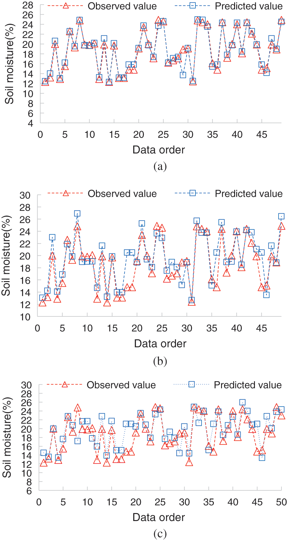
Figure 10: The prediction values of soil moisture in Daxing (a) Prediction values in 1 day (b) Prediction values in 3 days (c) Prediction values in 5 days
Table 5: Correlation coefficient of model testing
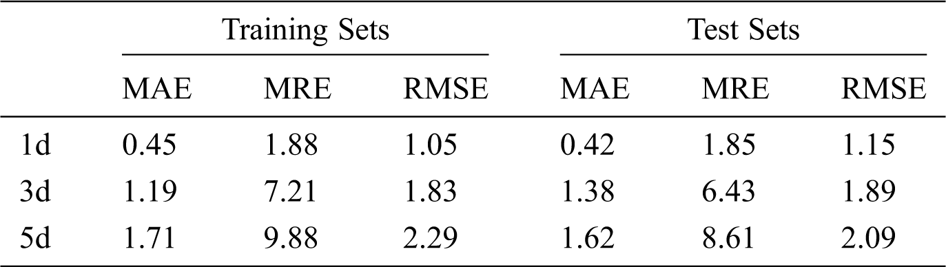
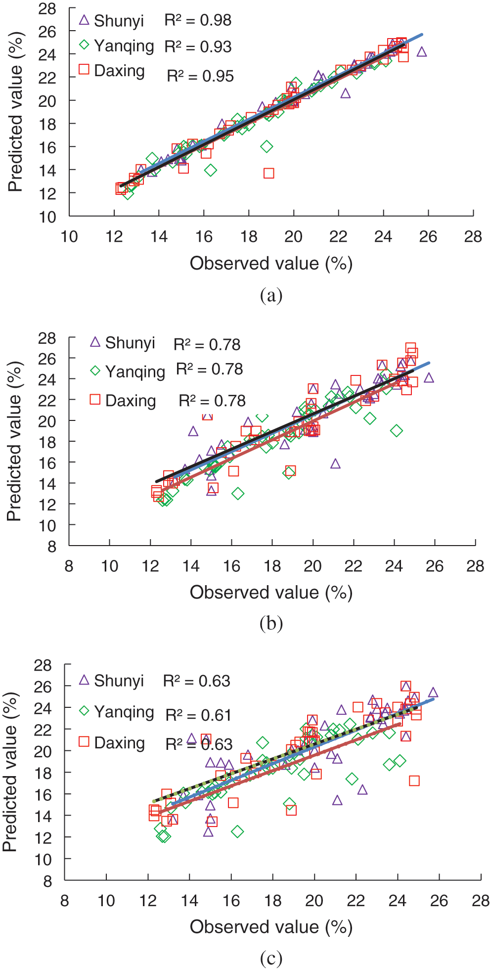
Figure 11: Correlation coefficient chart of model testing (a) Correlation coefficient in 1 day (b) Correlation coefficient in 3 days (c) Correlation coefficient in 5 days
In this paper, the GEP model is established with temperature, air pressure, humidity, wind speed, ground temperature, rainfall, and initial temperature values as the inputs of the model. About 1000 sets of data from Shunyi, Yanqing, and Daxing were used to train and calibrate the model. Furthermore, we evaluated the performance of the model. The results show that the GEP model based on seven factors can well realize the prediction of soil moisture. The prediction accuracy of soil moisture in different regions is different, as the soil conditions in different regions are different, for this reason, the prediction accuracy of the three regions is not the same. Among them, Shunyi area is common, but all of them are in an acceptable range, which proves that GEP has good generalization. With the increase in the prediction period, the prediction accuracy decreases. The prediction accuracy is the lowest for 5 days; because the prediction period is long, it has a large influence on the prediction results. In future research, we will further improve the dynamic update combined with real-time data to improve the long-range prediction accuracy.
Funding Statement: This work was supported by National Key R&D Program of China (2016YFD0300201-3, 2016YFC0403102), Innovation ability construction project of Beijing academy of agriculture and forestry sciences (KJCX20180703), and the modern Agro-Industry Technology Research System of Maize (CARS-02- 87).
Conflicts of Interest: The authors declare that they have no conflicts of interest to report regarding the present study.
1. J. Wang, Y. Cao, P. Zhang and L. Zhang. (2016). “Analysis of soil moisture variation characteristics in Yunnan Province,” Water Saving Irrigation, vol. 5, pp. 97–105. [Google Scholar]
2. D. Chen, G. Z. Wang and Q. Liu. (2019). “Multi-Scale variation prediction of PM2.5 concentration based on a monte carlo method,” Journal on Big Data, vol. 1, no. 2, pp. 55–69. [Google Scholar]
3. C. L. Li, X. M. Sun and J. H. Cao. (2019). “Intelligent mobile drone system based on real-time object detection,” Journal on Artificial Intelligence, vol. 1, no. 1, pp. 1–8. [Google Scholar]
4. St. Elmaloglou and N. Malamos. (2000). “Simulation of soil moisture content of a prairie field with SWAP93,” Agricultural Water Management, vol. 43, no. 2, pp. 139–149. [Google Scholar]
5. R. G. Perea, E. C. Poyato, P. Montesinos and J. A. RodríguezDíaz. (2019). “Optimisation of water demand forecasting by artificial intelligence with short data sets,” Biosystems Engineering, vol. 177, no. 2, pp. 59–66. [Google Scholar]
6. H. Zhou, Y. J. Chen and S. M. Zhang. (2019). “Ship trajectory prediction based on BP neural network,” Journal on Artificial Intelligence, vol. 1, no. 1, pp. 29–36. [Google Scholar]
7. J. C. Chen and Y. M. Wang. (2020). “Comparing activation functions in modeling shoreline variation using multilayer perceptron neural network,” Water, vol. 12, no. 5, pp. 1281–1293. [Google Scholar]
8. H. C. Jia, D. H. Pan, Y. Yuan and W. C. Zhang. (2014). “Using a BP neural network for rapid assessment of populations with difficulties accessing drinking water because of drought,” Human and Ecological Risk Assessment: An International Journal, vol. 21, no. 1, pp. 100–116. [Google Scholar]
9. P. J. Xu, C. Li, L. G. Zhang, F. Yang, J. Zheng et al. (2019). , “Underground disease detection based on cloud computing and attention region neural network,” Journal on Artificial Intelligence, vol. 1, no. 1, pp. 9–18. [Google Scholar]
10. W. C. Yang, S. H. Chon, C. M. Choe and U. H. Kim. (2019). “Materials selection method combined with different MADM methods,” Journal on Artificial Intelligence, vol. 1, no. 2, pp. 89–100. [Google Scholar]
11. Y. M. Zhai, A. D. Deng, J. Li, Q. Cheng and W. Ren. (2019). “Remaining useful life prediction of rolling bearings based on recurrent neural network,” Journal on Artificial Intelligence, vol. 1, no. 1, pp. 19–27. [Google Scholar]
12. Z. L. Yin, Q. Feng, L. S. Yang, R. Deo, X. H. Wen et al. (2017). , “Future projection with an extreme-learning machine and support vector regression of reference evapotranspiration in a mountainous inland watershed in North-West China,” Water, vol. 9, no. 1, pp. 1–23. [Google Scholar]
13. C. J. Huang, L. Li, S. H. Ren and Z. S. Zhou. (2010). Research of Soil Moisture Content Forecast Model Based on Genetic Algorithm BP Neural Network, vol. 345. Berlin Heidelberg: Springer, pp. 309–316. [Google Scholar]
14. C. H. Chen, J. Tan, J. K. Yin, F. Zhang and J. Yao. (2010). “Prediction for soil moisture in tobacco fields based on PCA and RBF neural network,” Transactions of the CSAE, vol. 26, no. 8, pp. 85–90. [Google Scholar]
15. S. Yuan, G. Z. Wang, J. B. Chen and W. Guo. (2019). “Assessing the forecasting of comprehensive loss incurred by Typhoons: A combined PCA and BP neural network Model,” Journal on Artificial Intelligence, vol. 1, no. 2, pp. 69–88. [Google Scholar]
16. T. Li, L. Y. Wang, Y. Chen, Y. J. Ren, L. Wang et al. (2019). , “A face recognition algorithm based on LBP-EHMM,” Journal on Artificial Intelligence, vol. 1, no. 2, pp. 59–68. [Google Scholar]
17. A. Pandey, S. K. Jha, J. K. Srivastava and R. Prasad. (2010). “Artificial neural network for the estimation of soil moisture and surface roughness,” Russian Agricultural Sciences, vol. 36, no. 6, pp. 428–432. [Google Scholar]
18. S. F. Quadri, X. Y. Li, D. S. Zheng, M. U. Aftab and Y. M. Huang. (2019). “Multi-Layer graph generative model using autoencoder for recommendation systems,” Journal on Big Data, vol. 1, no. 1, pp. 1–7. [Google Scholar]
19. P. Tiwari and P. Shukla. (2019). “A hybrid approach of TLBO and EBPNN for crop yield prediction using spatial feature vectors,” Journal on Artificial Intelligence, vol. 1, no. 2, pp. 45–59. [Google Scholar]
20. S. Samadianfard, E. Asadi and S. Jarhan. (2017). “Wavelet neural networks and gene expression programming models to predict short-term soil temperature at different depths,” Soil and Tillage Research, vol. 17, no. 2018, pp. 37–50. [Google Scholar]
21. S. Emamgolizade, S. M. Bateni, D. Shahsavani, T. Ashrafi and H. Ghorbani. (2015). “Estimation of soil cation exchange capacity using Genetic Expression Programming (GEP) and Multivariate Adaptive Regression Splines (MARS),” Journal of Hydrology, vol. 529, no. 6, pp. 1590–1600. [Google Scholar]
22. S. A. Razaq, S. Shahid, T. Ismail, E. S. Chung, M. Mohsenipour et al. (2016). , “Prediction of flow duration curve in ungauged catchments using genetic expression programming,” Procedia Engineering, vol. 154, no. 2–4, pp. 1431–1438. [Google Scholar]
23. M. Nematzadeh, A. A. Shahmansouri and M. Fakoor. (2020). “Post-fire compressive strength of recycled PET aggregate concrete reinforced with steel fibers: Optimization and prediction via RSM and GEP,” Construction and Building Materials, vol. 252, pp. 1–12. [Google Scholar]
24. S. Wang, Z. Y. Fu, H. S. Chen, Y. P. Nie and K. L. Wang. (2015). “Using Gene-expression programming method and geographical location information to simulate evapotranspiration in Hunan and Hubei Provinces,” Chinese Journal of Eco-Agriculture, vol. 23, no. 4, pp. 490–496. [Google Scholar]
25. S. Wang, Z. Y. Fu, H. S. Chen, Y. L. Ding, L. P. Wu et al. (2017). , “Simulation of reference evapotranspiration based on random forest method,” Transactions of The Chinese Society of Agricultural Machinery | T Chin Soc Agric Mach, vol. 48, no. 3, pp. 302–309. [Google Scholar]
 | This work is licensed under a Creative Commons Attribution 4.0 International License, which permits unrestricted use, distribution, and reproduction in any medium, provided the original work is properly cited. |