DOI:10.32604/iasc.2021.015225
| Intelligent Automation & Soft Computing DOI:10.32604/iasc.2021.015225 | |
| Article |
Weed Recognition for Depthwise Separable Network Based on Transfer Learning
1College of Information and Technology, Jilin Agricultural University, Changchun, 130118, China
2Changchun Institute of Engineering and Technology, Changchun, 130117, China
3Department of Biological Systems Engineering, Centre for Precision and Automated Agricultural Systems, Washington State University, Prossers, WA, 99350, USA
*Corresponding Author: Yang Zhou. Email: zhouyang@jlau.edu.cn
Received: 11 November 2020; Accepted: 22 December 2020
Abstract: For improving the accuracy of weed recognition under complex field conditions, a weed recognition method using depthwise separable convolutional neural network based on deep transfer learning was proposed in this study. To improve the model classification accuracy, the Xception model was refined by using model transferring and fine-tuning. Specifically, the weight parameters trained by ImageNet data set were transferred to the Xception model. Then a global average pooling layer replaced the full connection layer of the Xception model. Finally, the XGBoost classifier was added to the top layer of the model to output results. The performance of the proposed model was validated using the digital field weed images. The experimental results demonstrated that the proposed method had significant improvement in both classification accuracy and training speed in comparison of VGG16, ResNet50, and Xception depth models. The test recognition accuracy of the proposed model reached to 99.63%. Further, the training of each round time cost was 208 s, less than VGG16, ResNet50 and Xception models’, which were 248 s, 245 s and 217 s, respectively. Therefore, the proposed model has a promising ability to process image detection and output more accurate recognition results, which can be used for other crops’ precision management.
Keywords: Weed recognition; deep learning; depthwise separable convolutional neural network; transfer learning
Adequate agricultural products are an important prerequisite to sustain population growth. Although China's grain yield has grown steadily, there still exist some problems. Weeds in the seedling stage are harmful to the yield and quality of major crops, such as maize and wheat [1,2]. Also, weeds compete with crop seedlings for moisture, nourishment, light, and growth space, causing crops bad-harvest, diseases and insect pests spread, threatening the survival of the crops [3]. Currently, extensive, and large-scale spraying of herbicides is the main weed method of weeding. Unfortunately, deuced herbicides will destroy the ecological environment, consume resources, and affect food safety [4]. In intelligent agriculture precision spraying is one important weed control method, which can effectively control field weeds, utilize herbicides, and reduce pesticide residues [5–7]. During precise spraying, accurate weed identification is the precondition and key part. Therefore, it is necessary to propose a fast and accurate weed identification method under complex field conditions.
Crop and weed recognition methods mainly include manual recognition, remote sensing recognition and machine learning recognition [8]. Manual recognition is time-consuming, tedious, and low efficiency, and limited by the subjective experience of agricultural personnel. Remote sensing recognition used spatial and spectral information to distinguish weeds and overcame many drawbacks of manual recognition. However, the remote sensing method has low accuracy for small individuals and low-density weeds due to low resolution of remote sensing images [9]. Fast and accurate machine learning technology has been increasingly applied in weeds recognition field. In recent years, many researchers have reported on their work [10–15]. Rojas et al. [14] used principal component analysis (PCA) dimensionality reduction combining with support vector machine (SVM) algorithm to identify weeds based on the differences in color, texture and other features between vegetable and weeds, with accuracy higher than 90%. In terms of shape and texture features, Dongjian et al. [15] fused shapes, texture and fractal dimensions as weed features, then SVM and Dempster-Shafer (DS) evidence theory were used for weed recognition. These weeds recognition methods are all based on traditional machine learning methods. However, traditional machine learning methods are difficult to extract features due to manual selection and correction of features as well as poor generalization in solving the problem of weed recognition. Deep learning with prominent characterization ability can automatically extract deep features of images. Thus, the application of deep learning in the weed recognition field has become a prominent research direction [16–23]. Razavi et al. [22] proposed a new network architecture based on Convolutional Neural Networks (CNNs). It can identify plant types from image sequences that are collected from intelligent agricultural stations. The experimental results proved that new CNN model has better recognition performance than SVM classifier, Local Binary Pattern (LBP) and Gist (GIST). Alessandro et al. [23] used Convolutional Neural Networks (ConvNets or CNNs) to perform weed detection in soybean crop images, as well as discriminating between grass and broadleaf weeds, aiming to apply in the specific herbicide to weed detected.
Deep learning eliminated the feature extraction disadvantage in the traditional machine learning recognition method and achieved better recognition results. While deep neural network models usually require large sample data and time-consuming to ensure the model performance.
In addition, higher recognition and classification accuracy often requires huge labeled data. In contrast, when the amount of labeled data is small, the neural network model will be over-fitted, resulting in low recognition accuracy. Meanwhile, it is difficult to obtain sufficient labeled data in practice, as a result, the model will lack model training. In addition, transfer learning can transfer knowledge from existing field data to help model training in new fields, which provides the possibility for neural network model training with few data.
In this study, we propose a weed identification method using the deep separable convolutional network based on transfer learning. The method aimed to introduce and improve a lightweight network model-Xception model based on the transfer learning strategy, which was named TX-XGBoost.
The implementation process of the proposed model (TX-XGBoost) is shown in Fig. 1. Firstly, we performed the data augmentation and background segmentation on the weed dataset. Secondly, we replaced the full connection layer and Softmax module of Xception with the newly designed global average pooling layer and XGBoost classifier to construct a new network model. Thirdly, the weights and parameters of the Xception convolutional layer that has been trained on the ImageNet data set are transmitted and loaded into the convolutional layer of the new model. At last, weed images can be trained through the new model, and the trained new model can detect and recognize weed images.
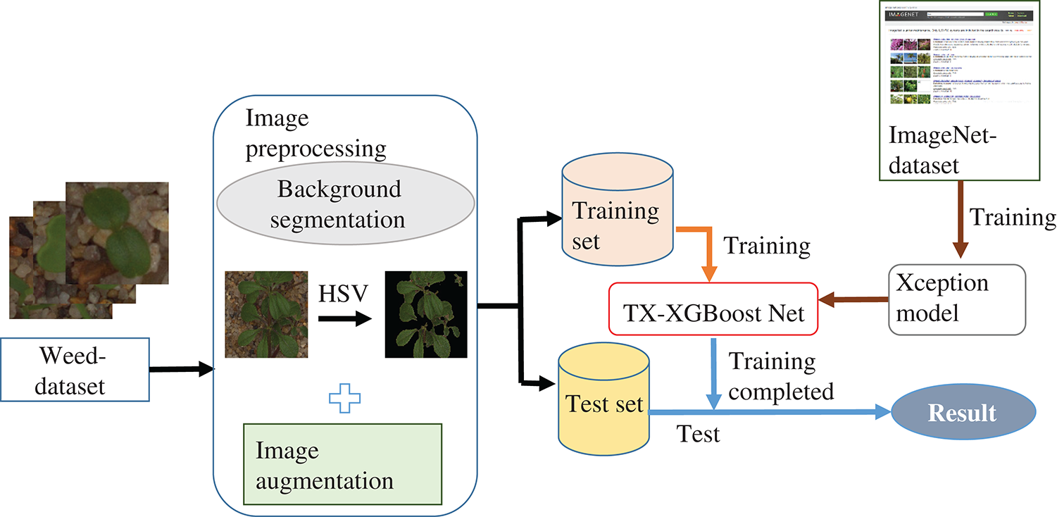
Figure 1: The schematic diagram of the weed recognition based on TX-XGBoost Net
In our experiment, all the weed images were from the publicly available database (https://vision.eng.au.dk/plant-seedlings-dataset/) that Southern Denmark University and Aarhus University jointly published. The data set consists of 4750 labeled RGB images in different sizes with a physical resolution of approximately 10 pixels per millimeter. The images contain three common crops of maize, wheat, sugar beet. Besides, the dataset also contains nine common field weeds such as Black-grass, Charlock, and Cleavers in natural backgrounds. As shown in Fig. 2, we displayed some image samples.
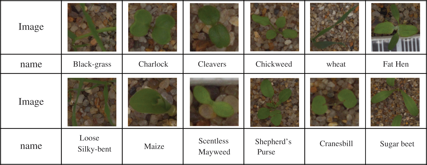
Figure 2: Some image samples
The images of field plants (crops and weeds) have complex backgrounds, such as soil and gravel, which could affect the model to extract valuable features. Therefore, to improve the recognition accuracy, it is necessary to segment the plant images and extract valuable features.
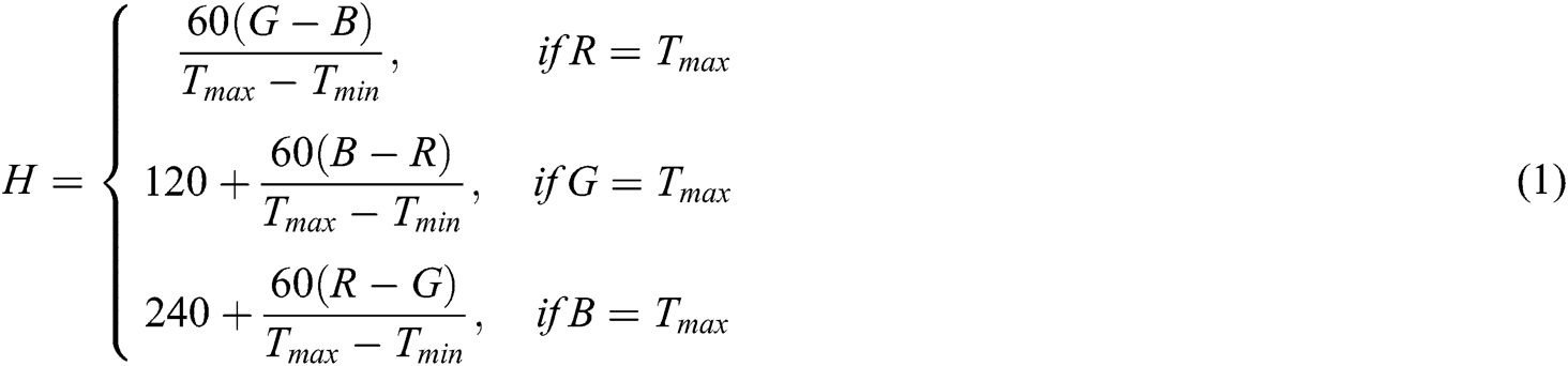
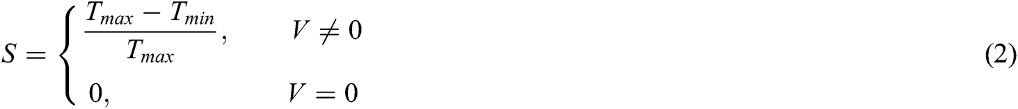
According to the green characteristics of seedling crops and weeds, we used the HSV-based green identification decision tree method [24]. This method can effectively segment plants and background, but also filtering processing. HSV (Here, H represents Hue. S and V is Saturation and Value, respectively) color space visually represents color hue, saturation, and brightness. It can accurately segment plants and backgrounds for tracking color information of an object easily. This method has stronger robustness compared with the Otsu algorithm, avoiding the influence on images of weather and time (such as brightness and contrast). OpenCV visual processing module in Python was used to convert the sample image from the RGB color space to the HSV color space. The conversion relationship is shown in the following equations:

where: R, G, B—pixel channel values of RGB color space
 —R, G, B maximum value
 —R, G, B minimum value
Plant HSV three-component threshold range was determined as the following steps: 1. Randomly selected 5 sample images from each species of plants to convert HSV color space. 2. Extracted 3 × 3 pixels from plants region in each image. 3. Calculated maximum and minimum values of each sample region to determine HSV three-component segmentation threshold range. According to this threshold, plants would be separated from non-target objects such as sand, rocks, debris, etc. Fig. 3(b) showed the binary image processed by HSV threshold segmentation, which contained uneven size holes due to the noise and lesions. Therefore, filtering processing was implemented on binary using morphological closing operation and Gaussian smoothing operation to obtain clear and complete segmented images. More importantly, the filtering operation was benefit to the network model training and classification. The filtered images shown in Figs. 3(c), and 3(d) were the final segmentation images.
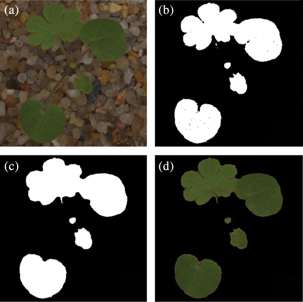
Figure 3: Background segmentation results of sample images. (a) Original image; (b) Binary image; (c) Filtered image; (d) Segmented image
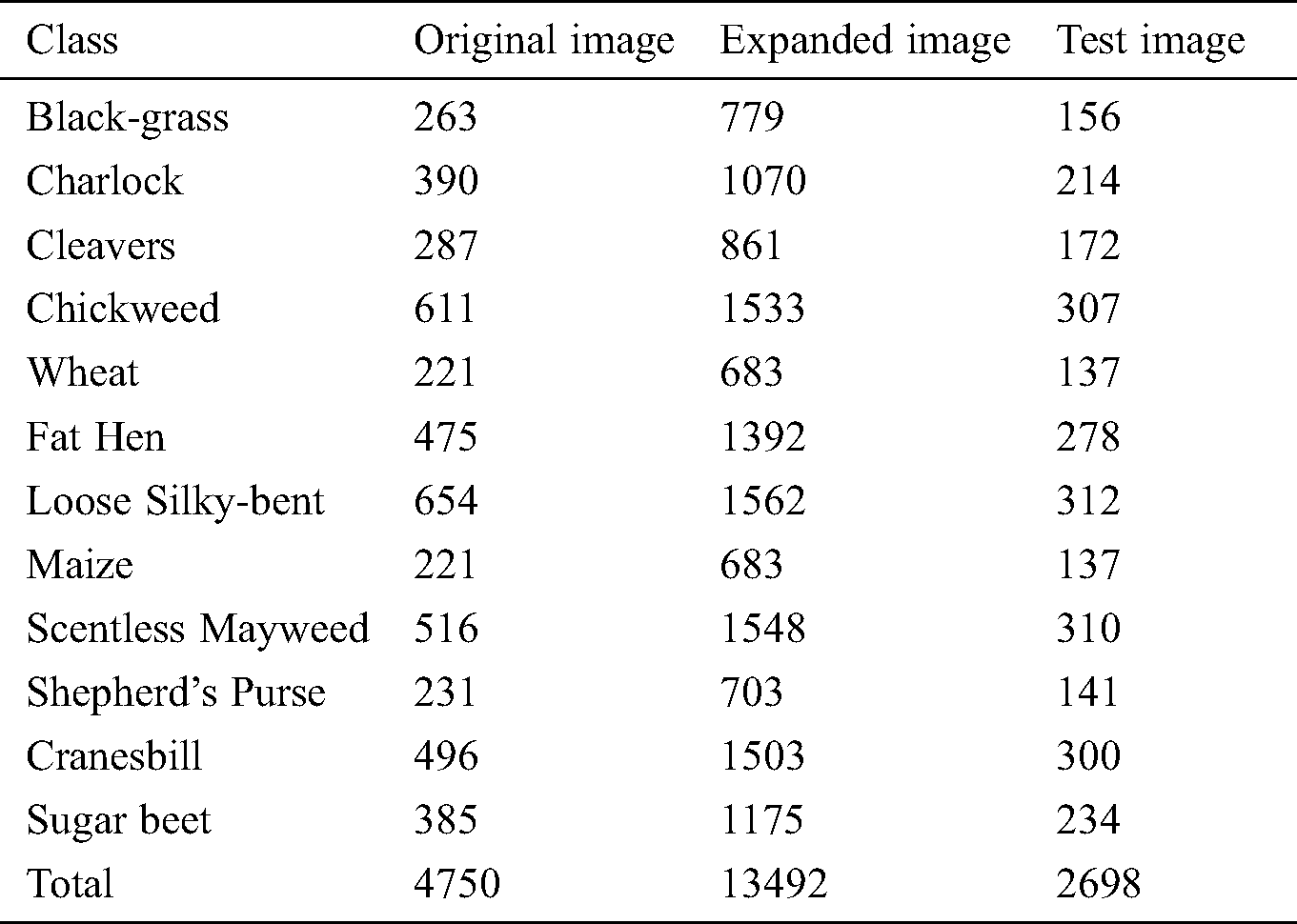
Good performance models require huge training data due to the deep learning model training is driven by big data [25]. Labeled samples in the dataset are few and difficult to meet the model training requirements. Therefore, data augmentation technique is introduced to expand the data to prevent over-fitting caused by insufficient samples. The model has good generalization ability, avoids the meaningless high-frequency feature of learning, and improves the network performance fundamentally. In this study, 80% of 4570 segmented and processed images were randomly selected for training and 20% for testing. Data augmentation included mirror flip, angle transformation (–20°~20°), random scaling (scaling factor 1~1.2), etc. The expanded training and testing samples were 10,794 and 2,698, respectively. The sample data distribution was shown in Tab. 1.
Table 1: Total number for initial and extended samples
2.3 Weed Recognition Network Model
2.3.1 Depthwise Separable Convolutional Neural Network
The core of a convolutional neural network is the convolutional layer. Increasing the number of convolutional layers tends to extract abundant feature information and improve the model performance due to the network properties. Convolutional networks have developed from the initial 7-layer AlexNet [26] to 16-layer VGG [27], then to 152-layer ResNet [28], and even to thousands of layers of DenseNet [29]. Although model performance has been improved, the gradient disappearance and training inefficiency also appeared, leading to model development difficultly as well as reducing identification rates. Google proposed a lightweight network model, Xception [30], which improved model performance without increasing network complexity.
The Xception model separated inter-channel correlation and spatial correlation mapping completely, which was the core conception of Xception called depthwise separable convolution. Traditional standard convolution applied convolution kernels to each channel of the input feature map and mapped spatial correlation and inter-channel correlation. However, depthwise separable convolution divided the standard convolution process into 2 steps, as shown in Fig. 4. Firstly, point wise convolution was performed on the input feature map, using 1 × 1 convolution kernel to map the cross-channel correlation. Secondly, depth wise convolution was performed mapping the spatial correlation of each output channel separately. Finally, the output feature map was obtained. This convolutional architecture extended the network width, extracted rich features, and effectively reduced the number of parameters comparing to the traditional standard convolution.
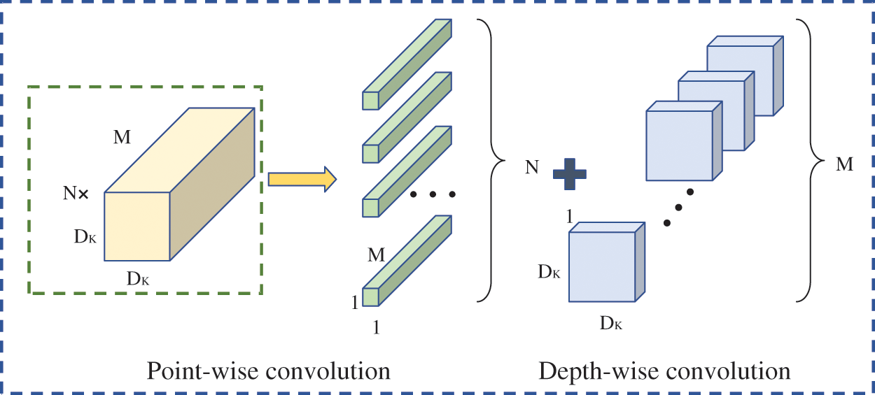
Figure 4: The schematic diagram of depthwise separable convolution
Assuming that the size of input feature map is , and the channel numbers are M; the output feature map size is the same as
 , and the channel numbers are N; the size of the convolution kernel is
 , the computation burden is
 according to the standard convolution. While, the computation burden for the point-by-point convolution and the depth convolution was
 and
and using depthwise separable convolution. The ratio of the computation burden of depthwise separable convolution to the standard convolution was calculated as follows:

The Eq. (4) shows that the calculation amount of depthwise separable convolution is related to the size of the convolutional core. The size of the convolution kernel used in Xception network model is generally 3 × 3 ( ), with many output channels (N). The computation amount of depthwise separable convolution could be derived from Eq. (4) to be about 1/9 of the standard convolution. Therefore, the storage of model weight parameters and the large amount of network calculation are greatly reduced.
In addition, Xception network model introduced a linear residual connection structure and a Batch Normalization (BN) layer to further accelerate the convergence of the network. Finally, network is classified by the Softmax classification layer and mapped to the probability space, which in turn outputs classification results. It should be noted that we chose the Xception convolutional layer as an image feature extractor to learn abstract features of images in this paper.
We modified the Xception model for reducing the model parameters and improving model classification accuracy. The steps included: (1) Replaced the full connection layer in the Xception model with a global average pooling layer. (2) Added an XGBoost classifier to the top layer of the model for classifying the data output.
• Global Average Pooling
Traditional convolutional neural networks used the full connection layer to reduce dimensions and perform non-linear transformation for high-dimensional feature data extracted from the convolutional layer, and the resulted data would be input into the classification layer for classification. This structure established a connection between the convolutional structure and the traditional neural network classifier. However, the full connection layer will cause parameter redundancy and over-fitting, which will affect the generalization ability of the network and result in needing more model training time.
Therefore, we replaced the full connection layer using the global average pooling layer [31] for reducing the number of parameters and the amount of computation and improving the model efficiency. Global average pooling was a regularization strategy, which averaged all the pixels of each feature map generated by the convolutional layer and obtained a low-dimensional feature vector. Compared with the full connection layer, the global average pooling layer enhanced the correspondence between the mapping features and the final category and retained the convolutional structure well. In addition, the global average pooling layer has no parameters to be optimized. Thus, the complexity of the model is reduced and the problem of over-fitting is avoided.
• XGBoost
Convolutional neural networks have an efficient feature extraction mechanism, which could classify images effectively and demonstrate their reliability. However, traditional classifiers cannot make full use of image information in image classification applications, and it is difficult to establish reliable recognition features. Therefore, for traditional classifiers, there is still much space for improvement in classification efficiency and accuracy.
XGBoost (eXtreme Gradient Boosting) classifier is on the top layer of the model to connect the global average pooling layer for classifying the images. In fact, XGBoost [32] is an integrated learning algorithm based on Boosting, a classification regression trees combination. It achieves accurate classification by converting weak classifiers into strong classifiers iteratively. The XGBoost algorithm introduces regularization to enhance generalization and performed second-order Taylor expansion on loss function. The integrated tree equation is as follows:

where —total number of submodels
 —the Kth tree model
 —predicted result of the sample
 —input characteristic of the sample
 —a set of all tree models
The introduced objective function was shown in Eq. (6):

where —regularization item
 —loss function, difference value between the predicted
  and actual
Transfer learning is to use the existing source domain knowledge to solve different but similar domain problems. The purpose is to transfer existing knowledge to help solve learning problems in the object domain with less training sampling images [33]. Aydin et al. [34] investigated the performance of the use of four different transfer learning models in deep neural networks on the plant classification results of four public datasets (Flavia, Swedish, UCI Leaf and PlantVillage). Experimental results show that transfer learning can improve plant classification performance. In the supervised training mode, transfer learning reduces the data usage for model training. It not only solves the model fitting problem caused by insufficient data in the target field, but also accelerates the convergence of the model, and improves the accuracy of the model.
The ImageNet dataset has more than 14 million labeled images and covers more than 20,000 categories. It is recognized as a “standard” data set for verification algorithms in the deep learning image field and currently widely used in the computer vision. Therefore, we combined transfer learning and deep learning to build a weed recognition network model. As shown in Fig. 5, it is a structure diagram of our TX-XGBoost model. Firstly, the Xception network model was used to pre-train the ImageNet data. Second, the trained convolutional layer weights and parameters were used as initialization parameters. Then the values obtained in second step were transfered to the convolutional layer of the TX-XGBoost model. Finally, weed dataset was used to fine-tune the parameters of the TX-XGBoost model to achieve generalization ability of the weed recognition model.
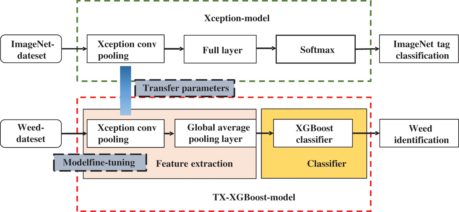
Figure 5: The schematic diagram of TX-XGBoost model. The traditional Xception-model is described in the green dotted box. Correspondingly, our TX-XGBoost model is shown in the red dotted box at the bottom of the schematic diagram
In our validation experiment, Python 3.6 using Keras library with Tensorflow backend was applied to build and train the TX-XGBoost network. The environment is Ubuntu 16.04 system, the server configuration is equipped with Intel Xeon E5-2680 v4 CPU, Samsung SSD 860 512 GB hard disk, Kingston DDR4 64 GB memory. The optimization made use of NVIDIA TITAN Xp GPU with 12 GB video memory to increase training speed.
Model training process had 3 steps as follows:
1. We resized the image into fixed-size 229 × 229 RGB image to reduce the dimension of training data and keep the details of the input image.
2. The batch size was 16, indicating each batch requires 16 samples to participate in training and update weight parameters once. The learning rate was 0.0001, and epoch was set 60. Besides, the modified CNN was trained using weed images on the Adam optimizer platform.
3. After the model convergence, resulting model automatically extracted features from the input sample data, as input of the XGBoost classifier. The completion of XGBoost training showed the end of the training of the entire model.
3.1 Recognition Results Analysis
The confusion matrix was presented to evaluate the performance of the classifier in weed identification, as shown in Fig. 6. The matrix rows and columns represent the true and predicted results respectively, and the values are expressed as percentages. Here it should be noted that Cleavers, Chickweed, wheat, Fat Hen, Scentless Mayweed, Shepherd’s Purse, Cranesbill and Sugar beet are accurately classified with accuracy of 100%. Charlock and Maize have 1.4% and 0.73% misclassification which are confused with Cleavers, Cranesbill and Scentless Mayweed, respectively. Black-grass is often confused with Loose Silky-bent of 2.56% misclassification rate, and Loose Silky-bent is sometimes confused with Black-grass because of similar morphological features. We can conclude that the TX-XGBoost has high recognition accuracy in weed recognition, and the overall recognition accuracy can reach 99.71%.
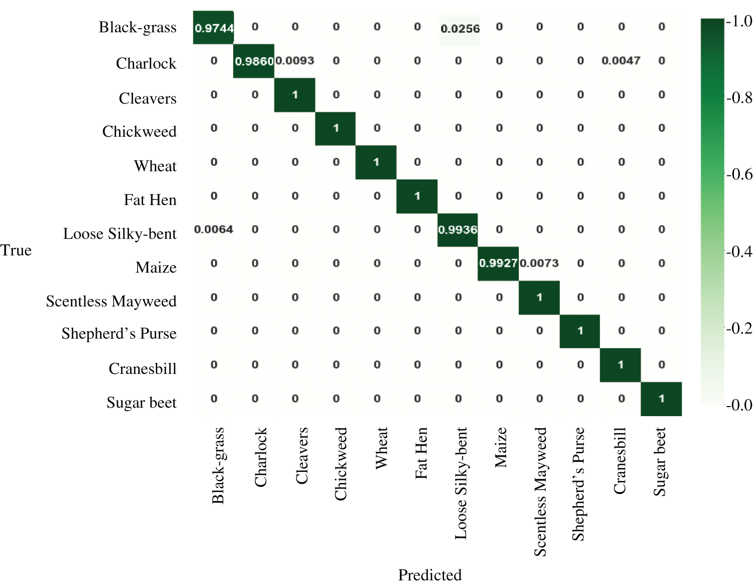
Figure 6: Accuracy evaluation using the confusion matrix
We used the statistical parameters of the confusion matrix (precision, recall, and F1-score) further analyze the performance of the classifier. Precision is the proportion of correct predictions to all predictions. The higher the value (closer to 1), the more accurate. Recall is the proportion of correct predictions to all positive predictions. Precision and recall can reveal accuracy and the completeness of the weed recognition. F1-score is harmotic average of precision and recall. Since precision and recall affect each other, F1-score can be used to balance them. The definition formulas of these three evaluation indexes are shown in Eqs. (7)–(9). Where True Positives (TP) is correct classification in positive class. False Positive (FP) is incorrect classification in positive class. True Negative (TN) is correct classification by negative class. False Negative (FN) is incorrect classification in negative class:


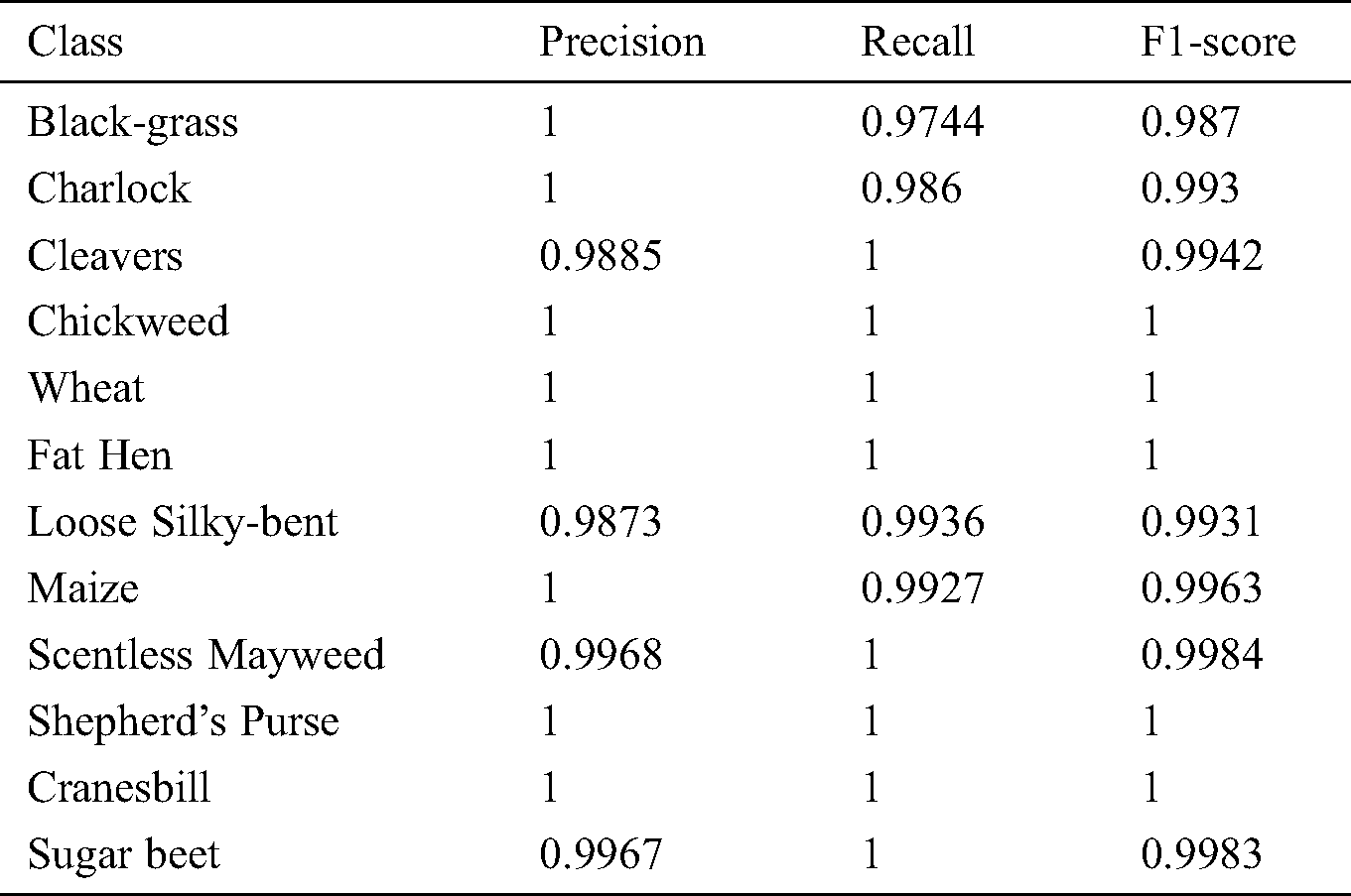
Tab. 2 shows three parameters’ values of TX-XGBoost model including precision, recall and F1-score. As shown in Tab. 2, the precision, recall and F1-score are 1 among the Chickweed, wheat, Fat Hen, Shepherd’s Purse and Cranesbill. And all scores of the classification reports are not lower than 0.97, which once again proves the superiority of TX-XGBoost model.
Table 2: Precision, recall and F1-score for the corresponding experimental configurations
3.2 Comparison with Other Models
The TX-XGBoost model was evaluated on the weeds dataset and compared it with the models including the VGG16, ResNet50, Xception under the same experimental environment. Meanwhile, the accuracy-fitting curves of the mentioned four methods under various epochs are shown in Fig. 7. It should be noted that Fig. 7(a) indicates the accuracy of training set. Correspondingly, Fig. 7(b) corresponds to test data. Observing Fig. 7(a), the accuracy will increase with more epochs and we can find that our model recognition accuracy is highest under different epochs. Especially, the accuracy of our model can reach 90% (when epoch equals to 5, as the red marked part in Fig. 7(a)), while the ResNet50 model needs ten epochs to reach the close recognition results, although ResNet50 has higher accuracy compared with VGG16 and Xception. Besides, the recognition of TX-XGBoost can reach to 99.78% under 60 epochs, and the ResNet50 can reach to 97.92%. Therefore, our proposed model can reduce the training epoch and improve training efficiency. As shown in Fig. 7(b), we can find that our model has best performance compared with other three models under the same epochs. As the accuracy of our model is 99.63% and ResNet50 is 97.17%. The accuracy of the proposed model can improve 2.46% in comparison with ResNet50. The above demonstrated results prove that TX-XGBoost has a better performance than other three models in the term of accuracy. It can also clarify that the transfer learning strategy and the improved network structure can accelerate the model convergence speed, thereby achieving higher accuracy.
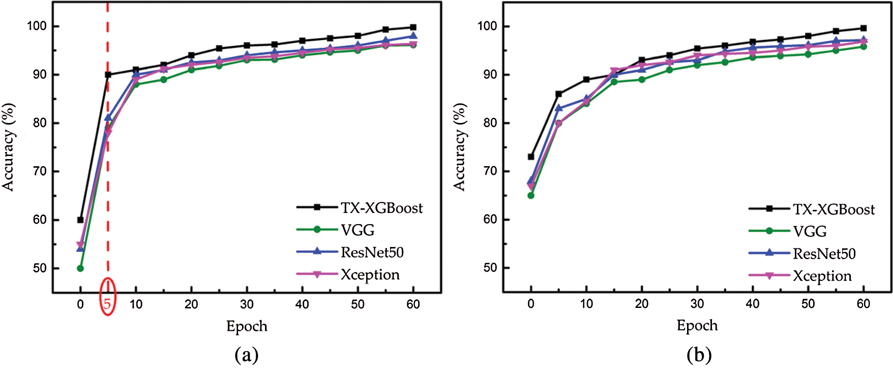
Figure 7: Plots of accuracy versus the different epochs based on different models. Black curves with squares and blue curves with triangles show the recognition accuracy of TX-XGBoost and RsNet50, respectively. Green curves with triangles and magenta curves with rounds correspond to the VGG and Xception recognition accuracy, respectively
Table 3: Performance comparison of different models in training set and test set
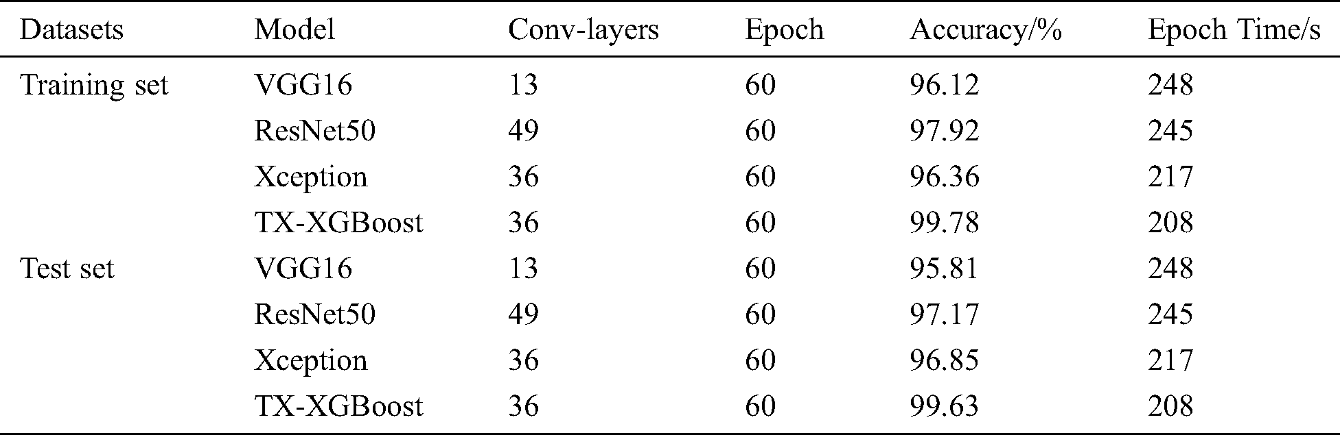
To further show the performance of TX-XGBoost, in 60 epochs, we compared the proposed model with other models regarding on running time. As shown in Tab. 3, ResNet50 model with 49 convolutional layers had better performance than VGG16 with 13 convolutional layers. For the Xception model, the training time was significantly reduced compared with that of VGG16 and ResNet 50, while the recognition accuracy is lower than the ResNet50 model. The proposed model can not only improve accuracy but reduce epoch time. Especially, the epoch time of TX-XGBoost model under training set was 208 s, less than VGG16, ResNet50 and Xception models’, which were 248 s, 245 s and 217 s, respectively. Besides, the number of convolutional layers of the proposed model was 13 layers which was less than that of ResNet50. The experimental results indicated that the proposed TX-XGBoost model can improve recognition accuracy and save computational time.
In this study, we proposed a novel weeds recognition model using depth wise separable convolutional neural network based on transfer learning. We introduced transfer learning into the model training, which solved the network over-fitting problem caused by insufficient training data and improved the generalization ability of the model. Meanwhile, to address the issue of large number of parameters and time-consumed training for conventional models, the lightweight model Xception was proposed and improved. The global average pooling layer was used to replace the full connection layer in the Xception model, and the XGBoost classifier was added to the top layer of the model to reduce the complexity of the model and improve the recognition accuracy of the model. The numerical experiment results demonstrated that our proposed model has advantages in accuracy and saving time compared with the traditional Xception, ResNet50 and VGG16 models. In the future, we will collect the experimental field data and establish weed data set to ensure the recognition accuracy of the proposed method in the practical application. Furthermore, the proposed method has broad applications in precision agriculture, such as weeding robots, pesticide spraying and other fields.
Acknowledgement: The authors wish to thank R. He who help to make experiments.
Funding Statement: This work is supported in part by the National Natural Science Foundation of China (http://www.nsfc.gov.cn/) under Grant 31801753, and the JiLin provincial science and technology department international exchange and cooperation project (http://kjt.jl.gov.cn/) under Grant 20200801014GH, and the Jilin province education department “13th five-year” science and technology research planning project (http://jyt.jl.gov.cn/) under Grant JJKH20200336KJ.
Conflicts of Interest: The authors declare that we have no conflicts of interest to report regarding the present study.
1. D. Avishek, U. Hayat, T. Nihat, P. Tosapon, C. B. Singh et al. (2017). , “Managing weeds using crop competition in soybean,” Crop Protection, vol. 95, pp. 60–68. [Google Scholar]
2. T. R. Chavan and A. V. Nandedkar. (2018). “AgroAVNET for crops and weeds classification: A step forward in automatic farming,” Computers & Electronics in Agriculture, vol. 154, pp. 361–372. [Google Scholar]
3. O. Alex, D. A. Konovalov, B. Philippa, R. Peter, J. Jamie et al. (2019). , “DeepWeeds: A multiclass weed species image dataset for deep learning,” Scientific Reports, vol. 9, no. 1, pp. 1–12. [Google Scholar]
4. H. H. Jiang, C. Y. Zhang, Y. L. Qiao and Z. Zhang. (2020). “CNN feature based graph convolutional network for weed and crop recognition in smart farming,” Computers and Electronics in Agriculture, vol. 174, pp. 105450. [Google Scholar]
5. K. Janc, K. Czapiewski and M. Wójcik. (2019). “In the starting blocks for smart agriculture: The internet as a source of knowledge in transitional agriculture,” NJAS-Wageningen Journal of Life Sciences, vol. 90, pp. 100309. [Google Scholar]
6. Y. L. Xu, R. He, Z. M. Gao, C. X. Li, Y. T. Zhai et al. (2020). , “Weed density detection method based on absolute feature corner points in field,” Agronomy, vol. 10, pp. 113. [Google Scholar]
7. K. Xiao, Y. Ma and G. Gao. (2017). “An intelligent precision orchard pesticide spray technique based on the depth-of-field extraction algorithm,” Computers & Electronics in Agriculture, vol. 133, pp. 30–36. [Google Scholar]
8. Z. K. Ke, X. Z. Yuan, D. S. Kun, C. C. Jian and W. Q. Feng. (2019). “Identification of peach leaf disease infected by Xanthomonas campestris with deep learning,” Engineering in Agriculture, Environment and Food, vol. 12, no. 4, pp. 388–396. [Google Scholar]
9. I. Sa, Z. T. Chen, M. Popovic, R. Khanna, F. Liebisch et al. (2018). , “WeedNet: Dense semantic weed classification using multispectral images and MAV for smart farming,” IEEE Robotics and Automation Letters, vol. 3, no. 1, pp. 588–595. [Google Scholar]
10. J. L. Tang, D. Wang, Z. G. Zhang, L. J. He, J. Xin et al. (2017). , “Weed identification based on K-means feature learning combined with convolutional neural network,” Computers & Electronics in Agriculture, vol. 135, pp. 63–70. [Google Scholar]
11. P. Lottes, M. Hörferlin and S. Sander. (2017). “Effective vision-based classification for separating sugar beets and weeds for precision farming,” Journal of Field Robotics, vol. 34, no. 6, pp. 1160–1178. [Google Scholar]
12. R. Raja, T. T. Nguyen and V. L. Vuong. (2020). “RTD-SEPs: Real-time detection of stem emerging points and classification of crop-weed for robotic weed control in producing tomato,” Biosystems Engineering, vol. 195, pp. 152–171. [Google Scholar]
13. Z. B. Wang, H. L. Li, Y. Zhu and T. F. Xu. (2017). “Review of plant identification based on image processing,” Archives of Computational Methods in Engineering, vol. 24, pp. 637–654. [Google Scholar]
14. C. P. Rojas, L. S. Guzmán and N. V. Toledo. (2017). “Weed recognition by SVM texture feature classification in outdoor vegetable crops images,” Ingeniería e Investigación, vol. 37, pp. 68–74. [Google Scholar]
15. D. J. He, Y. L. Qiao, P. Li, Z. Gao and J. L. Tang. (2013). “Weed recognition based on SVM-DS multi-feature fusion,” Transactions of the Chinese Society for Agricultural Machinery, vol. 44, no. 2, pp. 182–187. [Google Scholar]
16. M. Dyrmann, R. N. Rgensen and H. S. Midtiby. (2017). “RoboWeedSupport—Detection of weed locations in leaf occluded cereal crops using a fully convolutional neural network,” Advances in Animal Biosciences, vol. 8, no. 02, pp. 842–847. [Google Scholar]
17. S. F. Alessandro, M. F. Daniel, G. S. Gercina, P. Hemerson and T. F. Marcelo. (2019). “Unsupervised deep learning and semi-automatic data labeling in weed discrimination,” Computers and Electronics in Agriculture, vol. 165, pp. 0168–1699. [Google Scholar]
18. J. L. Yu, A. W. Schumann, Z. Cao, S. M. Sharpe and N. S. Boyd. (2019). “Weed detection in perennial ryegrass with deep learning convolutional neural network,” Frontiers in Plant Science, vol. 10. [Google Scholar]
19. J. L. Yu, S. M. Sharpe, A. W. Schumann and N. S. Boyd. (2019). “Detection of broadleaf weeds growing in turfgrass with convolutional neural networks,” Pest Management Science, vol. 75, no. 8, pp. 2211–2218. [Google Scholar]
20. M. Dyrmann, H. Karstoft and H. S. Midtiby. (2016). “Plant species classification using deep convolutional neural network,” Biosystems Engineering, vol. 151, pp. 72–80. [Google Scholar]
21. A. Wang, W. Zhang and X. Wei. (2019). “A review on weed detection using ground-based machine vision and image processing techniques,” Computers and Electronics in Agriculture, vol. 158, pp. 226–240. [Google Scholar]
22. S. Razavi and H. Yalcin. (2017). “Using convolutional neural networks for plant classification,” In 2017 25th Signal Processing and Communications Applications Conference, pp. 1–4. [Google Scholar]
23. D. S. F. Alessandro, M. F. Daniel, G. D. S. Gercina, P. Hemerson and T. F. Marcelo. (2017). “Weed detection in soybean crops using ConvNets,” Computers & Electronics in Agriculture, vol. 143, pp. 314–324. [Google Scholar]
24. W. Z. Yang, S. Wang, X. L. Zhao, J. S. Zhang and J. Q. Feng. (2015). “Greenness identification based on HSV decision tree,” Information Processing in Agriculture, vol. 2, no. 3–4, pp. 149–160. [Google Scholar]
25. A. Raphael, Z. Dubinsky, D. Iluz and N. S. Netanyahu. (2020). “Neural Network Recognition of Marine Benthos and Corals,” Diversity, vol. 12, no. 1, pp. 29. [Google Scholar]
26. A. Krizhevsky, I. Sutskever and G. Hinton. (2012). “ImageNet classification with deep convolutional neural network,” Advances in Neural Information Processing Systems, vol. 60, pp. 84–90. [Google Scholar]
27. K. Simonyan and A. Zisserman. (2014). “Very deep convolutional networks for large-scale image recognition,” arXiv preprint, arXiv: 1409.1556. [Google Scholar]
28. K. M. He, X. Y. Zhang, S. Q. Ren and J. Sun. (2016). “Deep residual learning for image recognition,” In Proceedings of the IEEE conference on computer vision and pattern recognition, pp. 770–778. [Google Scholar]
29. G. Huang, Z. Liu, V. D. M. Laurens and W. Killian. (2016). “Densely connected convolutional networks,” In Proceedings of the IEEE conference on computer vision and pattern recognition, pp. 4700–4708. [Google Scholar]
30. F. Chollet. (2016). “Xception: Deep learning with depthwise separable convolutions,” In Proceedings of the 22nd acm sigkdd international conference on knowledge discovery and data mining, pp. 785–794. [Google Scholar]
31. M. Lin, Q. Chen and S. Yan. (2013). “Network in network,” arXiv preprint, arXiv: 1312.4400. [Google Scholar]
32. T. Chen and C. Guestrin. (2016). “XGBoost: A scalable tree boosting system,” In Proceedings of the 22nd acm sigkdd international conference on knowledge discovery and data mining, pp. 785–794. [Google Scholar]
33. Z. F. Kang, B. Yang, Z. S. Li and P. Wang. (2019). “OTLAMC: An online transfer learning algorithm for multi-class classification,” Knowledge-Based Systems, vol. 176, pp. 133–146. [Google Scholar]
34. A. Kaya, A. S. Keceli, C. Catal, H. Y. Yalic, H. Temucin et al. (2019). , “Analysis of transfer learning for deep neural network based plant classification models,” Computers and Electronics in Agriculture, vol. 158, pp. 20–29. [Google Scholar]
 | This work is licensed under a Creative Commons Attribution 4.0 International License, which permits unrestricted use, distribution, and reproduction in any medium, provided the original work is properly cited. |