DOI:10.32604/iasc.2021.014437
| Intelligent Automation & Soft Computing DOI:10.32604/iasc.2021.014437 | |
| Article |
Building Graduate Salary Grading Prediction Model Based on Deep Learning
Department of Computer Science and Information Engineering, National Taipei University of Technology, Taipei, 106335, Taiwan
*Corresponding Author: Jong-Yih Kuo. Email: jykuo@ntut.edu.tw
Received: 20 September 2020; Accepted: 26 October 2020
Abstract: Predicting salary trends of students after employment is vital for helping students to develop their career plans. Particularly, salary is not only considered employment information for students to pursue jobs, but also serves as an important indicator for measuring employability and competitiveness of graduates. This paper considers salary prediction as an ordinal regression problem and uses deep learning techniques to build a salary prediction model for determining the relative ordering between different salary grades. Specifically, to solve this problem, the model uses students’ personal information, grades, and family data as input features and employs a multi-output deep neural network to capture the correlation between the salary grades during training. Moreover, the model is pre-trained using a stacked denoising autoencoder and the corresponding weights after pre-training are used as the initial weights of the neural network. To improve the performance of model, dropout and bootstrap aggregation are used. The experimental results are very encouraging. With the predictive salary grades for graduates, school’s researchers can have a clear understanding of salary trends in order to promote student employability and competitiveness.
Keywords: Neural network; deep learning; ordinal regression problem; stacked de-noising auto-encoder
In recent years, research on graduate employment trends has been one of the main research focuses on institutional researchers. In 2015, the Statistics Bureau at Ministry of Education in Taiwan [1] conducted employment tracking of Ph.D., master, bachelor, and college graduates from 2010 to 2012, with the purpose of strengthening employment counseling, shortening the gap in learning and the allocation of educational resources. It collects personal information about graduates, personal income, resignation records, military insurance, and employment insurance records. The statistics department then uses statistical analysis to study the direction of graduates, industry distribution, average monthly salary, etc. However, there is still very little research on salary grades. Therefore, based on the deep learning method and the 2011–2015 academic year graduates of Taipei University of Technology as the research object, this paper established a salary grade prediction model.
The rest of this paper is organized as follows. Section 2 provides concise literature reviews, such as ordinal regression, stacked de-noising auto-encoder, bootstrap aggregating, and related educational data mining case. Section 3 introduces the research design and describes the data processing and data analysis methods. The system design and implementation are also described. Section 4 presents and discusses the empirical results. Section 5, the final section, concludes the paper with the listing of the contributions and limitations of this study.
In this section, we first review the methods used for data preprocessing and related literature. Therefore, the methods in the literature can be divided into ordinal regression problem settings, stacked de-noising auto-encoders, and Bootstrap Aggregating integrated learning algorithms. In the second part of this section, we reviewed the concepts and theoretical models related to mining cases with relevant educational data.
Ordinal regression is a supervised learning problem aiming to classify instances into ordinal categories [2–5]. It is used to solve the problem of classification and when used, target categories are not usually independent of one another as they have a specific order relationship. Ordinal regression, also called, ‘rank’, is evident in sequences such as the scoring items in a questionnaire (strongly agree, agree, not sure, disagree, strongly disagree), students’ grades (A, B, C, D, E), education levels (elementary school, junior high school, senior high school, university), age (per years), etc. There is a sequence relationship in this type of categories and the difference in the spacing between the categories may be inconsistent.
Niu et al. [6] propose using of an End-to-End learning approach to address ordinal regression problems using deep Convolutional Neural Network, which could simultaneously conduct feature learning and regression modeling. In particular, an ordinal regression problem is transformed into a series of binary classification sub-problems. And propose a multiple output CNN (Convolutional Neural Network) learning algorithm to collectively solve these classification sub-problems so that the correlation between these tasks could be explored.
Chang et al. [7] propose an approach that fully utilizes a well-ordered set of relationship labels. Given a well-ordered set of labels, such as human ages, the approach separates the labels into two groups based on the following ordering property: larger than and no larger than a label k. Hence, they proposed to convert by exploiting this property, can form K-1 sub problems, which are considerably less complex than the K(K-1)/2 setting.
2.2 Stacked De-Noising Auto-Encoder
Srivastava et al. [8] proposed the concept of Auto-encoder, which is a type of artificial neural networks with two parts: Encoder and decoder. The main purpose of the Auto-encoder is to learn efficient representations of the input data, called coding, without any supervision. The Auto-encoder uses loss function to measure the error between the input data and the reconstructed data.
When data contain noise, the model easily indicates overfitting; besides, the impact of noise on the model is more intense where there is a small amount of data. Therefore, Vincent et al. [9] proposed De-noising Auto-encoder (DAE). The DAE adds artificial noise to input data before encoding so that the neural network can learn from the data with noise to reconstruct the original data. It can eliminate noise and reduce the impact of noise on the neural network model.
Vincent et al. [10] proposed the concept of using a Stacked De-noising Auto-encoder (SDAE) to initialize a deep neural network. The principle is to stack DAE to build a deep architecture and use unsupervised learning for training each layer of DAE. After the current L-layer training is completed, the L+1 layer is trained using the weight of the former L layer. SDAE can be used as input for supervised learning algorithms, or using the optimization method of training, to add a layer of the network at the end of SDAE. Because the weight of the network is initialized by SDAE, this training process is called the fine-tune process.
Bootstrap Aggregating is a kind of Ensemble Learning algorithm. This algorithm can be used in the classification or regression model. Bootstrap Aggregating random sampling effectively reduces the noise and outlier in datasets and to avoid overfitting, reduces the impact of noise on the model. Fig. 1 shows the process of the Bootstrap Aggregating algorithm. Firstly, the training dataset randomly picks the N dataset and then builds the N model. Each model corresponds to one dataset and this dataset is used for training. Finally, these models can be regarded as basic predictors. When the model deals with a regression problem, the final prediction result is the average of all model predictions; and when the model deals with a classification problem, the final prediction result is obtained via voting.
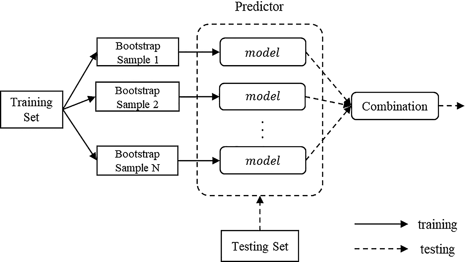
Figure 1: Bootstrap aggregating
2.4 Related Educational Data Mining Case
In a study, reference [11] used a deep neural network model to predict students’ course scores. It used the K-Means algorithm to classify the courses and build a model for each course for different academic years. The model also built a base predictor for different years using the Ensemble Learning concept and each predictor was pre-trained with a Stacked De-noising Autoencoder. Compared with SVM, Random Forest, and Linear Regression, the model has a higher performance, with an accuracy level of 89.62%.
The study [12] used Stacked De-noising Autoencoder for model pre-training, using the students’ personal data and average score per semester as input features to predict the probability of dropout [8]. The prediction result is used to counseling and warn students which be dropout likely and then reduced the unnecessary resource of school.
3 Design of the Salary Grading Prediction Model
The salary grading prediction model design process is divided into three: data preparation, construction of a deep network model, prediction, and evaluation. The details are shown in Fig. 2.

Figure 2: Model design flow char
College and master’s students who graduated in the 2011–2015 academic year from the National Taipei University of Technology (NTUT) comprise the data source for this study. The input features are given in Tab. 1. The output feature is the salary grading for one (1) to three (3) years after graduation, obtained from the Insured Salary Grading of Labor Insurance. In order to accommodate the change in the minimum wage (the Labor Insurance Bureau adjusted the minimum grading level yearly), we adjusted it to a consistent level for all the years under study.
This study excluded unemployed, uninsured, and part-time employees from its data. We classified those who were insured for less than 30 days and those with less than 20,100 salary grading as part-time employees. Due to the data size constraints, this study merged the data into nine categories. Fig. 3 shows the frequency of original salary grading, it indicates an insignificant frequency of low salary grades. Subsequently, Fig. 4 shows the merged salary grading frequency. The merged salary grading data shows a more balanced distribution in each grading group.


Figure 3: Salary grading data (Original)

Figure 4: Salary grading data (merge)
3.1.1 Data Integration and Cleaning
Data quality has a significant influence on model predictions [13]. The preprocessing of the data in this study was divided into three types: feature scaling, data encoding, missing values, and outlier processing.
Feature Scaling
Different value ranges of data may lead to slow convergence and predictive performance degradation during model training. In this study, the characteristics of the numerical data were normalized (Min-Max Normalization) so that the distribution of the input features had an interval scale [0,1]. The formula is as follows:

Data Encoding
Non-numerical data must be encoded into a numerical form before it can be inputted into the neural network model. This study performed One-Hot Encoding on the unordered non-numerical data and Label Encoding on the ordered non-numerical data.
Deal with missing data and outlier
Missing values affect the performance of a model. Sun et al. [14,15] proposed an improved method of concatenating transfer edges. By using the character interval, several consecutive characters are represented by character intervals, which can reduce the number of transfer edges effectively Hence, this study used three treatments for missing values. For non-numerical data, we added a category; and for numerical data, we used the average of all the data in that field. If the data row had many missing values, it was discarded. In this study, the data was converted into the Box Plot to determine the outliers and extreme values. If the outliers and extreme values had special significance, then they were kept. Otherwise, the data were consciously deleted.
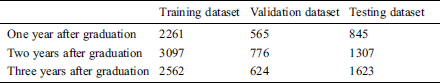
This study divided the data into training dataset, validation dataset, and testing dataset. It used the latest academic year’s data as a testing dataset to ensure the generalization of the model. 80% of the remaining data was used as a training dataset, while 20% of the remaining data was used as a validation dataset. The details of the count data are shown in Tab. 2.
3.2 Build a Deep Neural Network
This study built neural networks for each year after graduation. We used three (3) layers of fully connected neural networks and an output layer based on the multiple output layer framework proposed by Niu et al. [6]. Our network architecture is presented in Fig. 5. There are 500–700 neurons in its hidden layers, and the number of output blocks is determined by the number of target feature categories.

Figure 5: Network architecture
The traditional neural network usually uses 0 or a value close to 0 as the initial weights, which makes the deep network tend to converge to the local minimum. Apart from this, when there are few data, the noise is very influential to the model, thus making the model easily indicate overfitting. This study used a Stacked De-noising Auto-encoder to pre-train weights so that it could reduce the probability of the model convergence to the barest minimum and thus, effectively reduce the impact of noise on the model. Our model pre-training process is shown in Fig. 6. We used mean square error as the loss function of DAE.
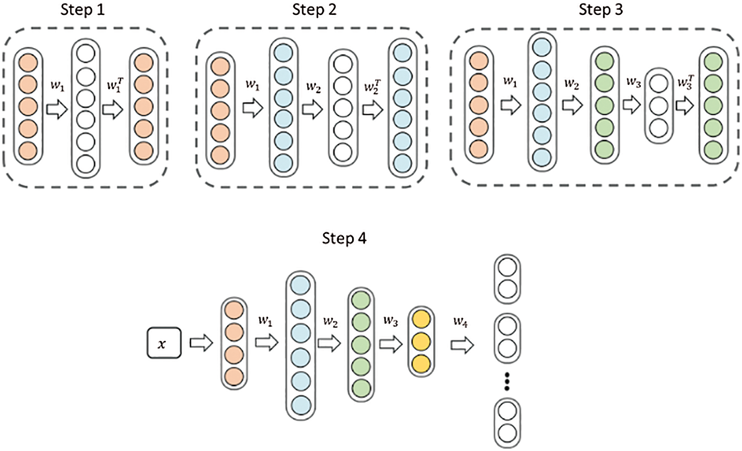
Figure 6: Pre-training process
3.2.2 Deep Neural Network Training
This study used pre-trained weights as the initial weights of the neural network. The output layer used a multiple output layer framework proposed by Niu et al. [6]. To implement this architecture, it was necessary to convert the nine salary grading’s into eight binary classification tasks’ target features. The conversion result is shown in Fig. 7 below. When the salary grading is 20.1 k, the value of the eighth target feature is 0. When the salary grading is 22.8 k, the value of the first target feature is 1, and the other target features are 0, and so on.

Figure 7: Target feature transformation
As shown in Fig. 8, this study used binary cross- entropy as a loss function to evaluate the error between the predicted and actual values of each task. Imbalanced data may cause the network model to prefer to predict the category which has more data, so, the loss of each task must be multiplied by the Task Importance Weight parameter, giving higher weight to categories with fewer data. Finally, this study used the Adam optimization method to fine-tune the network layer parameters.
When the model is too complex, it is easy to cause the model to over-fit the training data and reduce the generalization ability. Hence, this study used L2 regularization to measure the complexity of the model and to reduce the weight value of the unimportant model. It further used Dropout to prevent the neurons from cooperating with each neural. Finally, this study used early stopping to immediately stop training when the validation loss is not reduced. The network training algorithm is given in Fig. 9.
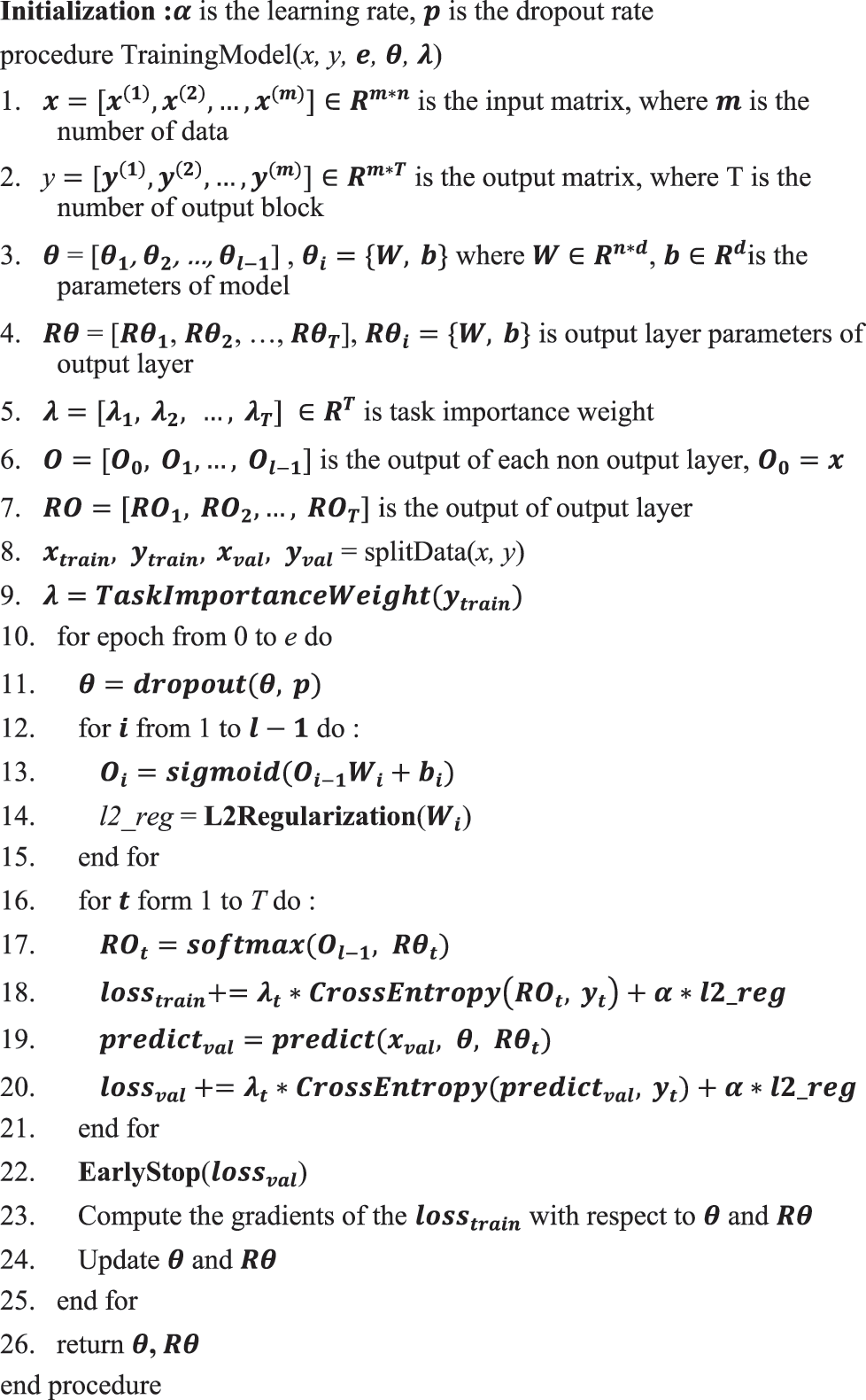
Figure 8: Deep neural network training

Figure 9: Network training algorithm
3.2.3 Bootstrap Aggregating Training
To improve the generalization ability of the model, this study used the Bootstrap Aggregating algorithm to train multiple neural networks. As shown in Fig. 10, this study randomly picked five (5) sets of training datasets and trained five (5) network models. In the prediction stage, the prediction result was selected by voting. The algorithm is given in Fig. 11.

Figure 10: Bootstrap aggregating training

Figure 11: Bootstrap aggregating training algorithm
4.1 Evaluation Measure for Ordinal Regression
For the ordinal regression problem, the standard method for measuring performance is MAE (Mean Absolute Error) [16]. The MAE is an average of the difference between all the predicted results and the actual results. The formula is as shown in Eq. (2), where N is the number of data, and y is the actual results, f(x) represents the model prediction results.

However, the ordinal regression problem is prone to feature imbalance in the categories. Baccianella et al. [17] showed that MAE performed very poorly at measuring performance when the ordinal categories that they tested were imbalanced. So, they proposed a macro-averaged MAE to solve the problem, this gives equal weight to all categories, to avoid the effects of imbalance. The researches [18–21] propose a prediction method that does comprehensively consider user preferences in complex environments, this method works by first calculating the disutility function value of the user to reflect his or her sensitivity to environmental changes; this disutility value is applied to the logarithmic model representing user preferences to calculate user route selection probability.
This study used the macro-averaged MAE; it is represented as MAE^M. The formula is as shown in Eq. (3).

4.2 Compare Performance with Use and Unused Pre-Training
Using SDAE for pre-training can reduce the dimensionality and impact of noisy data. This experiment compared performance between using and without using pre-training, to understand whether the model has better performance after pre-training.
Fig. 12 shows the unused pre-training model that had a higher loss in the early epoch, and the convergence speed was slower. Although the training loss was decreased, the validation loss increased after 3000 epochs, which means that the model begins overfitting. The use of pre-training had a lower loss in early epochs; the training loss and the validation loss were closer. So, the use of pre-training has better generalization capabilities.

Figure 12: Compare performance with use and unused pre-training
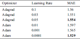
This study compared the number of different network layers with the number of neurons to find the number of hidden layers and neurons that were most suitable for the model. As shown in Tab. 3, two hidden layers had the best performance, neuron 700 and 500. This study compared different optimization methods and learning rates and found the best optimization method and learning rate for model efficiency. Tab. 4 shows the results of different optimization methods and learning rates. The method proposed by Adam obtained the lowest error when the learning rate is 0.0001. Therefore, this study used Adam as the model optimization method and set the learning rate to 0.0001.
Table 3: Layer and neural experiment
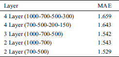
Table 4: Optimizer and learning rate experiment
4.4 Compare with Other Algorithms
This study compared the predictive performance of four machine learning algorithms, SVM, SVR, Logistic Regression (LR), Random Forest (RF), and Ordinal Regression (OR). Our model uses dimension reduction to solve the problem of excess input dimension and little data in the training process. Apart from this, the machine learning model uses PCA (Principal Component Analysis) dimension reduction method, but our proposed model has a lower MAE than other machine learning models. The results are shown in Tabs. 5 to 7. Our model’s confusion matrixes are shown in Figs. 13 to 15.
The regression algorithm, SVR, has lower MAE than our model in the first year after the students graduated, but it has poor results on the data of two or three years after the students graduated. This is due to the imbalance of data, most of the data fall behind the grading so that the regression algorithm does not predict the first few grading.
Use the two-three-year model of students after graduation instead of using the salary grade data of previous years as input features, which makes the prediction result to have a better performance after 25.6 K grading. However, the data of two or three years after the student’s graduate is extremely imbalanced and there is only a small amount of data so that there is not enough data for the first few grading to train. It can be seen from Figs. 14 and 15 that the prediction results of the first two grading are more scattered.
Table 5: Performance comparison result of our model (a year after graduated)
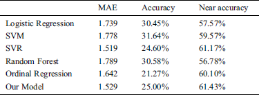
Table 6: Performance comparison result of our model (two years after graduated)

Table 7: Performance comparison result of our model (three years after graduated)
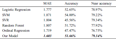
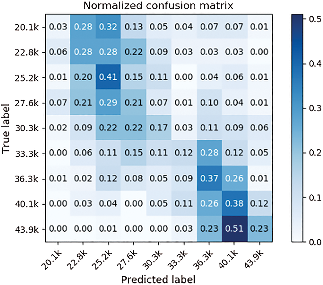
Figure 13: Confusion matrix (a year after graduated)
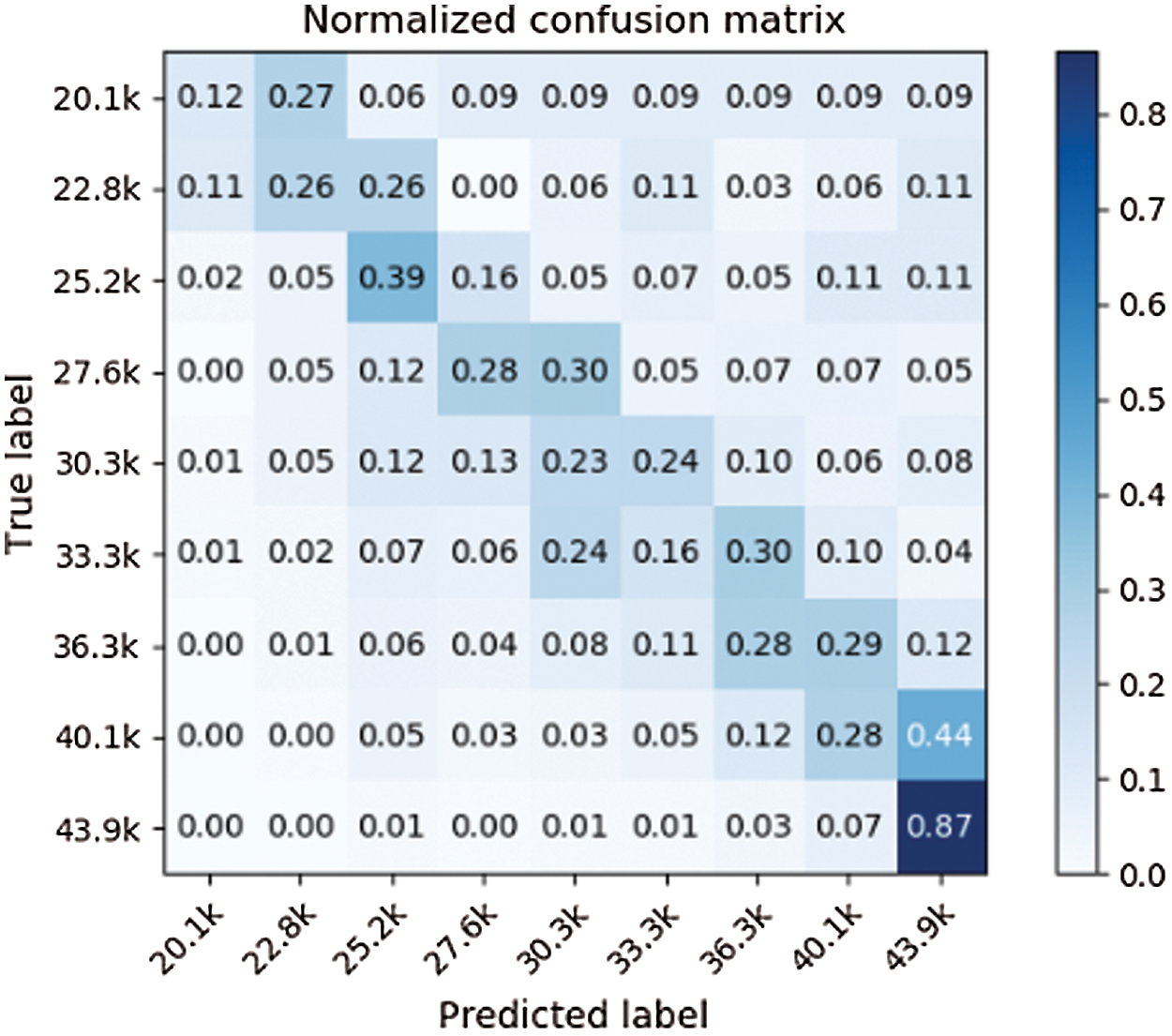
Figure 14: Confusion matrix (three years after graduated)
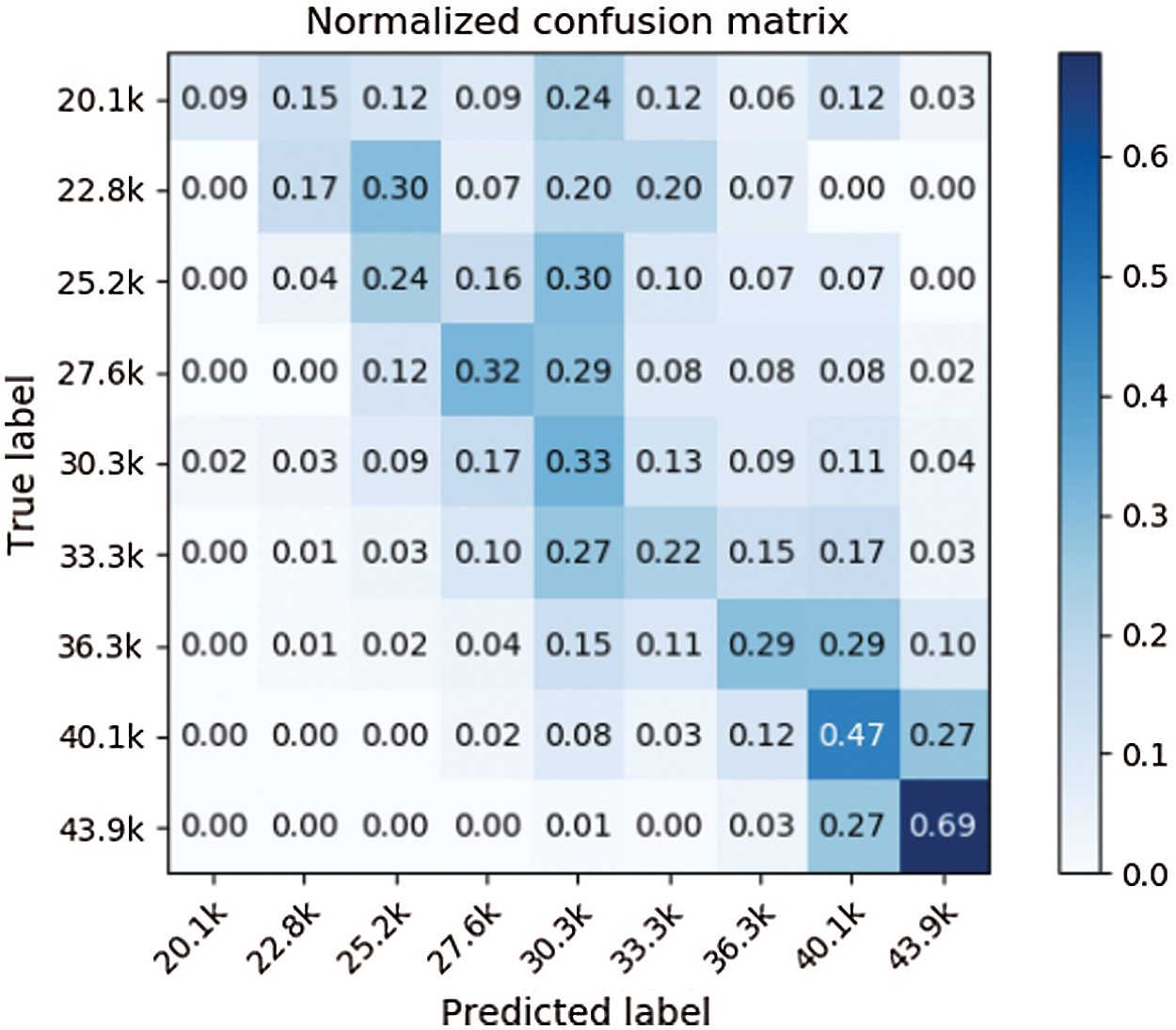
Figure 15: Confusion matrix (two years after graduated)
This study used deep neural network, which is a lower MAE than machine learning method, to predict graduates’ salary grading. The study built a salary grading prediction model by ordinal regression, which can be extended to other ordinal data type prediction problems, such as students’ Grade Point Average (GPA) prediction. The proposed model provides relevant information on salary trends to the school’s researchers who can use this information to provide the corresponding strategy to help raise the students’ salary of students when they are employed.
Funding Statement: This research was supported by Ministry of Science and Technology, R.O.C. under the Grant No. MOST 106-2221-E-027-018-MY2. The author J.Y. Kuo received the grant, and the URLs of sponsor’s website is https://www.most.gov.tw/.
Conflicts of Interest: The authors declare that they have no conflicts of interest to report regarding the present study.
1. Department of statistics of Ministry of Education, R.O.C. (2019). “99-101 Academic year institutions of higher education graduate’s employment salary big data analytics,” , [Online]. Available: https://depart.moe.edu.tw/ED4500/Content_List.aspx?n=E316EA4999034915. [Google Scholar]
2. Y. Z. Liu, A. W. K. Kong and C. K. Goh. (2018). “A constrained deep neural network for ordinal regression,” in Proc. of the IEEE Conf. on Computer Vision and Pattern Recognition, Salt, USA, pp. 831–839. [Google Scholar]
3. P. He, Z. L. Deng, C. Z. Gao, X. N. Wang and J. Li. (2017). “Model approach to grammatical evolution: Deep-structured analyzing of model and representation,” Soft Computing, vol. 21, no. 18, pp. 5413–5423. [Google Scholar]
4. J. M. Zhang, W. Wang, C. Q. Lu, J. Wang and A. K. Sangaiah. (2020). “Lightweight deep network for traffic sign classification,” Annals of Telecommunications, vol. 75, no. 7–8, pp. 369–379. [Google Scholar]
5. Shuren Zhou and BoTan. (2019). “Electrocardiogram soft computing using hybrid deep learning CNN-ELM,” Applied Soft Computing, vol. 86, 105778. [Google Scholar]
6. Z. Niu, M. Zhou, L. Wang, X. Gao and G. Hua. (2016). “Ordinal regression with multiple output CNN for age estimation,” in Proc. of the IEEE Conf. on Computer Vision and Pattern Recognition, Las Vegas, USA, pp. 4920–4928. [Google Scholar]
7. K. Chang, C. Chen and Y. Hung. (2011). “Ordinal hyperplanes ranker with cost sensitivities for age estimation,” in Proc. of the IEEE Conf. on Computer Vision and Pattern Recognition, Colorado, USA, pp. 585–592. [Google Scholar]
8. N. Srivastava, G. E. Hinton, A. Krizhevsky, I. Sutskever and R. Salakhutdinov. (2014). “Dropout: A simple way to prevent neural networks from overfitting,” Journal of Machine Learning Research, vol. 15, pp. 1929–1958. [Google Scholar]
9. P. Vincent, H. Larochelle, Y. Bengio and P. A. Manzagol. (2008). “Extracting and composing robust features with denoising autoencoders,” in Proc. of the 25th Int. Conf. on Machine Learning, Helsinki, Finland, pp. 1096–1103. [Google Scholar]
10. P. Vincent, H. Larochelle, I. Lajoie, Y. Bengio and P. Manzagol. (2010). “Stacked denoising autoencoders: Learning useful representations in a deep network with a local denoising criterion,” Journal of Machine Learning Research, vol. 11, pp. 3371–3408. [Google Scholar]
11. J. Y. Kuo, H. C. Lin, H. T. Chung, P. F. Wang and B. Lei. (2021). “Building student course performance prediction model based on deep learning,” Journal of Information Science and Engineering, vol. 37. no. 1, pp. 1–14. [Google Scholar]
12. J. Y. Kuo, C. W. Pan and B. Lei. (2017). “Using stacked denoising autoencoder for the student dropout prediction,” in proc. of the 2017 IEEE Int. Sym. on Multimedia. Taichung, 483–488. [Google Scholar]
13. W. J. Li, Y. X. Cao, J. Chen and J. X. Wang. (2017). “Deeper local search for parameterized and approximation algorithms for maximum internal spanning tree,” Information and Computation, vol. 252, pp. 187–200. [Google Scholar]
14. R. X. Sun, L. f. Shi, C. Y. Yin and J. Wang. (2019). “An improved method in deep packet inspection based on regular expression,” Journal of Supercomputing, vol. 75, no. 6, pp. 3317–3333. [Google Scholar]
15. C. Y. Yin, H. Y. Wang, X. Yin, R. X. Sun and J. Wang. (2019). “Improved deep packet inspection in data stream detection,” Journal of Supercomputing, vol. 75, no. 8, pp. 4295–4308. [Google Scholar]
16. L. Gaudette and N. Japkowicz. (2009). “Evaluation methods for ordinal classification,” in Proc. of the 22nd Canadian Conf. on Artificial Intelligence, kelowna, Canada, pp. 207–210. [Google Scholar]
17. S. Baccianella, A. Esuli and F. Sebastiani. (2009). “Evaluation measures for ordinal regression,” in Proc. of 9th Int. Conf. Intelligent System, pp. 283–287. [Google Scholar]
18. Z. Q. Xia, Z. Z. Hu and J. P. Luo. (2017). “UPTP vehicle trajectory prediction based on user preference under complexity environment,” Wireless Personal Communications, vol. 97, no. 3, pp. 4651–4665. [Google Scholar]
19. Y. Song, Y. Zeng, X. Y. Li, B. Y. Cai and G. B. Yang. (2017). “Fast CU size decision and PU mode decision algorithm for intra prediction in HEVC,” Multimedia Tools and Applications, vol. 76, no. 2, pp. 2001–2017. [Google Scholar]
20. J. J. Ren, S. Zhao, J. D. Sun, D. Li and S. Wang. (2018). “PPP: Prefix-based popularity prediction for efficient content caching in content-centric networks,” Computer Systems Science and Engineering, vol. 33, no. 4, pp. 259–265. [Google Scholar]
21. G. E. Hinton and R. R. Salakhutdinov. (2006). “Reducing the dimensionality of Data with neural networks,” Science, vol. 313, no. 5786, pp. 504–507. [Google Scholar]
 | This work is licensed under a Creative Commons Attribution 4.0 International License, which permits unrestricted use, distribution, and reproduction in any medium, provided the original work is properly cited. |