DOI:10.32604/iasc.2020.011853
| Intelligent Automation & Soft Computing DOI:10.32604/iasc.2020.011853 | |
| Article |
Hybrid Imperialist Competitive Evolutionary Algorithm for Solving Biobjective Portfolio Problem
1Department of Mathematics, Baoji University of Arts and Sciences, Baoji, 721013, China
2Center for Big Data Research in Languages/School of English Studies, Xi’an International Studies University, Xi’an, 710071, China
3School of Aerospace, Transport and Manufacturing, Cranfield University, Cranfield, MK43 0AL, UK
*Corresponding Author: Chun’an Liu. Email: liu2006@126.com
Received: 01 June 2020; Accepted: 22 July 2020
Abstract: Portfolio optimization is an effective way to diversify investment risk and optimize asset management. Many multiobjective optimization mathematical models and metaheuristic intelligent algorithms have been proposed to solve portfolio problem under an ideal condition. This paper presents a biobjective portfolio optimization model under the assumption of no short selling. In order to obtain sufficient number of portfolio optimal solutions uniformly distributed on the portfolio efficient Pareto front, a hybrid imperialist competitive evolutionary algorithm which combines a multi-colony levy crossover operator and a simple-colony moving operator with random perturbation is also given. The performance of the given algorithm is verified by four criterion portfolio test problems, and the simulation results and comparison analyses illustrate that the proposed algorithm could obtain faster convergence toward the portfolio true Pareto front compared with the other two state of the art multiobjective optimization methods. The results can provide optimal portfolio plans and investment strategies for investors to allocate and manage assets effectively.
Keywords: Portfolio optimization; biobjective mathematical model; imperialist competitive algorithm; asset management
Diversified investment is a well-practiced approach to avoid investment risk and obtain maximum portfolio return [1]. How to select and allocate limited capital in financial management and portfolio field is still one of the most challenging and important problem [2]. A pioneering portfolio optimization model, called mean-variance (M–V) model was addressed by Markowitz [3], which laid the foundation for modern financial theory. The M–V model has significant application value, and it provides insightful perspective for the research of the investment return and risk of portfolio optimization problems. In fact, M–V portfolio model is usually considered as a simple-objective portfolio optimization model which aims at minimizing the investment risk or maximizing the return of the capital. Therefore, M–V model made significant contribution for the development of modern finance and portfolio theories, and it is deemed as a classical method for the measurement of the performance of portfolio optimization problems [4–7].
Since the publication of Harry M. Markowitz’s M–V portfolio theory, it has gained widespread application and promotion as a practical mathematic method for portfolio optimization, and large amount of publications modifying or extending the portfolio optimization models and developing new effective portfolio optimization algorithms have been found [8,9]. Generally speaking, we can classify portfolio models into simple-objective portfolio optimization and multiobjective portfolio optimization. As far as simple-objective portfolio model (problem) is concerned, many researches usually minimize the variance of the portfolio while satisfying the bound of a portfolio return and the threshold of the invested assets in the portfolio optimization [10–12].
For the past few years, several metaheuristic intelligence evolution methods have been extended and used to solve multiobjective portfolio optimization in financial and economic fields. For example, Fernandez et al. [13] put forward a hybrid metaheuristic optimization algorithm to handle multiobjective project portfolio optimization problems; Li et al. [14] jointly presented a multiobjective portfolio selection optimization model and genetic algorithm based on fuzzy random returns; Lwin et al. [15] focused on solving complex constrained portfolio optimization and proposed a learning-guided multiobjective algorithm; Anagnostopoulos and Mamanis built a three objectives discrete portfolio model [16], and Deng et al. [17] discussed the multiobjective portfolio problem with a vision of intuitionistic fuzzy set, and so on [18,19].
Imperialist competitive algorithm (ICA) [20] is an intelligence optimization algorithm similar to the particle swarm method and the fish swarm algorithm, which has been used to solve the complex practical problems. As we know, ICA possesses polynomial convergent velocity or convergent order and can easily jump out the constraint of local convergence. For example, an ICA for solving nonlinear dynamic simple-objective constrained optimization problems is introduced in [21], and an enhanced ICA for optimum design of skeletal structures is given in [22], etc.
To reduce the complexity of the algorithm due to the non-smooth quadratic property of Markowitz’s mean-variance model and find a reasonable intelligent method in solving portfolio optimization, this research presents a biobjective portfolio mathematical model with no short selling. Also, a hybrid imperialist competitive evolutionary algorithm combining a multi-colony levy crossover operator and a simple-colony moving operator with random perturbation is proposed to obtain sufficient uniformly distributed and representative portfolio optimal solutions on the portfolio effective Pareto frontier. The numerical simulations are made on four standard portfolio problems, the simulation results show that the given hybrid ICA is effective in solving multiobjective portfolio optimizaiton problem and can obtain better portfolio optimal solutions.
The rest of the paper is arranged as follows. Section 2 is related concepts and biobjective portfolio model. The main operators of the proposed hybrid ICA to solve biobjective portfolio model are given in Section 3. Section 4 is the detailed procedure of the given algorithm. Section 5 is the simulation result and experimental analysis, and the conclusion is made in Section 6.
2 Related Concepts and Biobjective Portfolio Optimization Model
To describe the biobjective portfolio model, related terminologies of multiobjective optimization are briefly introduced in the following subsection.
2.1 Multiobjective Optimization
An unconstrained multiobjective minimized optimization problem is described as follows:

where  is decision variable,
  , and
, and

is called feasible region.
The objective vector  which contains m objectives maps the feasible region
  into objective space of problem (1). All feasible solutions of multiobjective programming problem (1) constitutes the Pareto optimal solution set, and the images of these feasible solutions form efficient Pareto front of problem (1).
Definition 1. Reference [23] Suppose  and
and  are two multi-dimensional vectors; if
  ,
,  and
and  for at least one index
  hold; then, vector
  is said to dominate vector
  (denoted as
  ).
).
Definition 2. Reference [23] Solution  is defined as Pareto optimal solution of problem (1); if not exists solution
  , and
, and  dominates
  .
.
Definition 3. Suppose that  are Pareto optimal solution sets obtained by
  algorithm
  , respectively. Then, solution set

is regared as a Pareto optimal filtration set.
2.2 Biobjective Portfolio Optimization Model
Classical portfolio optimization model, such as Markowitz’s M–V portfolio selection model, assumes n available assets and one investment period. The investor can choose the proportion weights of the initial investment which will be allocated in the available assets. In fact, Markowitz’s M–V portfolio model can be regarded as a single-objective portfolio mathematical model. The prevalent method dealing with the M–V optimization model is either to minimize risk (variance) of security while constraining return of security to a lower level, or to maximize the return of security (mean) while controlling risk of security in a ceiling level. The biobjective portfolio optimization model described in this section is based on two measures: one is the portfolio risk measure function and the other is the non-positive function of portfolio return.
Suppose that  is the column vector of portfolio,
  is the i-th investment proportional weight of security, we define
  as a history return value of the i-th security at the t-th phase (
 ), and
  as investment expected return value of the i-th security, then, function

is defined as a measure of portfolio risk, and non-positive function

is taken as a measure of portfolio return; then, we define

as a new biobjective portfolio model, where  is decision vector,
  is n-dimension search space, and

 is the tight constraint, where the constraints condition (7) indicates that short selling is not allowed for biobjective portfolio optimization problem (6).
Definition 4 Suppose that pop(k) presents the evolution country population of the k-th generation,  and
and  is the number of these feasible points (individuals) which dominate
  in country population pop(k), and
  are
are  feasible individuals which dominate the feasible individual
  . Denote

where  can be regarded as the accumulation rank value of individual
  .
.
3 Main Operators of Imperialist Competitive Algorithm
ICA [20] contains a population of countries and mimics the social and political competition process of imperialism. In the competition, some best original individuals (countries) were chosen to constitute the original imperialists, and the rest of countries were regarded as colonies of the original imperialist according to reasonable rules. Then, each of original imperialists with its colonies was called an empire. The competitive behavior will carry out among all the empires. If an empire could not win among the competition, it would become the colony of the strongest imperialist. Thus, all the colonies will move to the imperialist associated with it. At last, this collapse mechanism makes all colonies converge to Pareto optimal solution. The detailed pseudo-process of ICA is described in the following part.
Compared with other artificial intelligence optimization algorithm, ICA begins with the initial evolution country population. One generates Npop initial countries based on the orthogonal design method [24]. Denote these initial countries as  , where
  ; then, the cost of each
  is defined as follows:

Choose  better countries with smaller accumulation rank from the initial evolution population to compose the initial imperialists, and the rest
  countries would be the colonies allocated into these imperialists according to their powers, which can be calculated by the formula (8). Thus, every empire has got a certain number colonies. Fig. 1 illustrates the process in detail.

Figure 1: Generating the initial imperialists and colonies
Mark each imperialist as  and each colony as
  , where
  and
and  . At the same time, we assign those colonies to different imperialists using the method of proportion selection according to their power and generate the initial empires.
Step 1: Based on the following formula (10), compute the normalized power for each of imperialists,

where  is normalized cost of
  , and
, and  is normalized power of
  , where
  ,
,  is accumulation rank value of
  , where
  . The imperialist which has less accumulation rank value will have more normalized cost value.
Step 2: Based on the following formula, we obtain a positive integer

where  represents the number of the colonies in the k-th imperialist, and
  represents the amount of the colonies.
Step 3: Randomly choose  colonies and assign them to
  , these colonies and
  constitute the k-th empire (denoted as
  ,
,  ). The initial imperialist and colonies of each empire are showed in Fig. 1 with different colors, and it is clearly shown that the more power an imperialist has, the bigger its relevant area of hexagon.
3.2 Simple-Colony Moving Operator with Random Perturbation
In practice, all the imperialists attempt to expand and develop their colonies by means of assimilation and force their colonies to approach them. When the colony moving method mentioned in [20] is used, it is difficult to make portfolio Pareto optimal solutions quickly converge the portfolio true Pareto frontier and also maintain the otherness and diversity of the country population. Considering the characteristics of biobjective portfolio optimization model proposed in subsection 2.2, a simple-colony moving operator with random perturbation is given.
Step 1: Assume  are
are  colonies included in the j-th empire, we make
  move to its relevant imperialist along the direction which is a vector connecting point
  and
and  , where
  is the stopping position of
  ’s moving. This movement step is modeled in Fig. 2 from
  to
to  in which the colony moves to the imperialist by s units, i.e.,

Figure 2: Moving  toward their relevant

where parameter s is the uniformly distributed random variable,  is the expansion coefficient, and
  , parameter
  causes
  to approach
  from both sides.
Step 2: Give a random number  ; if
; if  hold, generate the new moving position
  of
of  according to the following random perturbation operator, i.e.,

where  is the k-th component of
  .
.  represents Gaussian distribution,
  . This movement step is modeled in Fig. 2 from
  to
to  in which the
  makes normal random perturbation operator and gets the new position
  of the initial
  .
.
3.3 Position Change between Imperialist and Colony
When a colony approaches an imperialist and acquires a new position, it may achieve a better fitness function than that of the imperialist. In this case, we can replace the imperialist with the colony, and vice versa. The proposed algorithm will continue to use this new colony as an imperialist. The detailed description can be found in [20,21].
3.4 Multi-Colony Levy Distribution Crossover Operator
How to make algorithm quickly converge to the portfolio efficient Pareto front and maintain the diversity of the population is critical for multiobjective portfolio method. In order to find new feasible solution region and further improve the robustness and diversity of the empire, a multi-colony levy distribution crossover operator is proposed in the following section.
Step 1: Select  colonies (denoted as
  ) from the
  , where
  .
.
Step 2: Let  , where
  .
.
Step 3: Carry out multi-colony levy distribution crossover operator, generate the offspring  of
of  , i.e.,

 is the random number satisfying levy distribution,
  ,
,  is the unit vector,
  ,
,  is the random normal distribution in which its mean is 0 and variance is 1, and n is the number of dimensions of the colony,
  ,
,  ,
,  .
.
For ICA [20], imperialistic competition plays an important role. During the competition process, weaker imperialists (own high accumulation rank value) will lose their colonies, and their power will begin to wane; meanwhile, the power of those stronger empires will begin to increase. The imperialistic competition process can be described as follows:
(1) Let  represent the power probability of the k-th empire; then,
  is defined as follows:

where  , imperialist* represents the imperialist of the k-th empire,
  represents the number of the colonies included in the k-th empire.
(2) Based on the following formula (16), generate power probability value  of every
  for
for  , i.e.,

 .
. represents the power probability of the k-th empire.
(3) Compute the cost (rank value) of each colony, and give these costs an ascending order. Then, we select  colonies from large to small in order and assign them to each empire according to its probability of power, let

and generate random vector  with uniformly distributed elements, i.e.,

where  for
for  . Furthermore, let

Let  . If
. If  hold, we can assign the
  selected from the
  colonies mentioned above into the j-th empire; otherwise, delete the
  , where
  .
.
3.6 Eliminating the Powerless Empires
During the process of competition, the colonies of weaker empire will be less and less. Finally, when an empire becomes powerless, it will be eliminated. To model this mechanism, we consider an empire collapses when it loses all of its colonies and the imperialist itself becomes a colony of another empire.
The competition operator will continue until each of the empires, except the strongest empire (lowest accumulation rank value), collapses and every colony included in the evolution population is controlled by this empire. That is to say, all the colonies have obtained the same costs (lower accumulation rank value) as the powerful empire. Under the circumstance, we stop the imperialist competition and output these portfolio Pareto optimal solutions whose accumulation rank value are equal to 1.
4 Hybrid Imperialist Competitive Evolutionary Algorithm
The proposed hybrid evolutionary algorithm (denoted in DPEA) for solving the biobjective portfolio optimization problem (6) is described as following:
Step 1: Give initial country size  and initial imperialist size
  . Generate
  initial countries
  based on the orthogonal design method [24] in the search space
  . Then, all of the initial countries constitute set
  , and let
  .
.
Step 2: Compute the accumulation rank value of these initial countries which is included in set  , and denote all of the countries whose accumulation rank value is equal to 1 as set
  and let
  .
.
Step 3: Select  powerful countries based on the power of each country and allocate the rest of the countries into them, and then, generate
  initial empire, i.e.,
  ,
,  .
.
Step 4: Let each colony among the empire approach the imperialist according to the simple-colony moving operator with random perturbation in Section 3.2, and exchange the position of the imperialist and the best colony included in the empire.
Step 5: Perform the multi-colony levy distribution crossover operator proposed in Section 3.4 and imperialistic competition operator proposed in Subsection 3.5, and generate the next country population  .
.
Step 6: Find out the countries which accumulation rank value are equal to 1 in set  , use them to replace those individuals included in set
  , and constitute new set
  .
.
Step 7: If the stopping criterion meets, output these Pareto optimal solutions in the external set  ; otherwise, return to Step 3.
5 Simulation Result and Analysis
To compare the effectiveness and robustness of DPEA with other advanced multiobjective intelligent computation algorithms, three classical performance metric indicator methods, C-measure [24], H-measure [25] and U-measure [26], are cited, where C-measure is usually used to test the domination of the portfolio Pareto optimal solutions obtained by two different multi-objective optimization methods, H-measure is used to assess whether the optimal solutions obtained by one multiobjective optimization algorithm is better than that of the other, and the third measure (U-measure) is used to test the augmentability and uniformity of these solutions distributed on Pareto front.
Furthermore, we choose four benchmark portfolio optimization problems  (
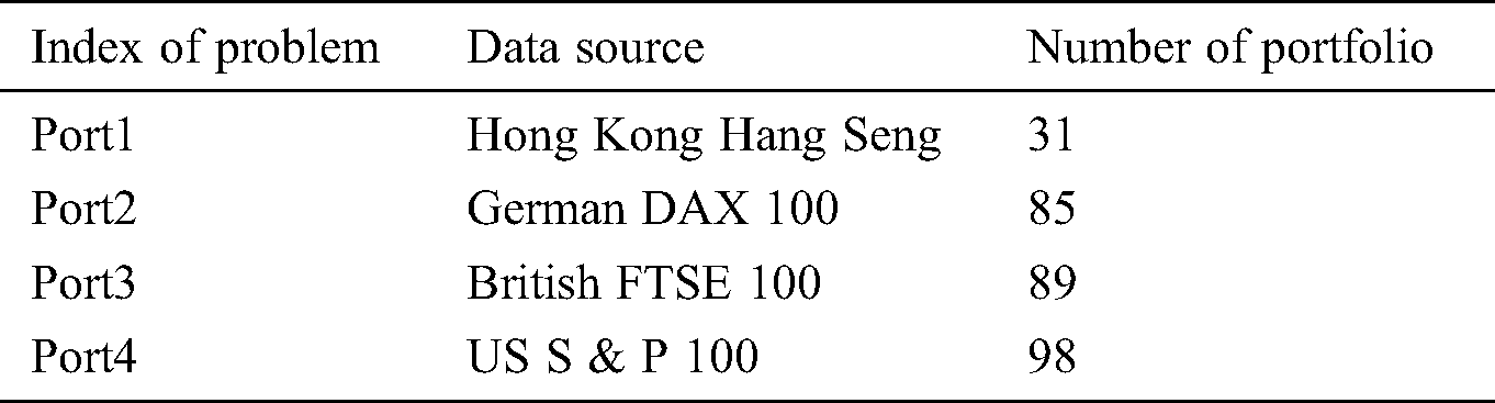
( ), in which the data of the mean, the variance and the correlation covariance matrix come from the Web of OR-library (http://people.brunel.ac.uk/~mastjjb/jeb/info.html). The index of test problems, the data source and the number of portfolio asserts are described in Tab. 1.
Table 1: Basic data of the test problems
It’s impossible to make an absolute equitable comparison result among the same kinds of algorithm based on no free lunch theorem. Thus, the identical test parameters are used in the simulation for both our algorithm DPEA and the other compared algorithms. Each benchmark portfolio problems were tested by two superior multiobjective methods DFEA [19], DCEA [23] and the proposed method DPEA. We implement each of algorithms on an Intel Pentium IV 2.8-GHz personal computer, and each test problems was carried out 30 runs using MATLAB 7.0. During the process of numerical test, the initial population (countries) size  , the initial stronger countries (imperialists) size
  , and the maximum iterations of algorithm is 200. Moreover, in order to test the sensitivity of parameter r mentioned in formula (15) for the algorithm’s performance and the quality of Pareto portfolio optimal solution obtained by the compared algorithms, we execute three algorithms, DFEA, DCEA, and DPEA, on each test problem at different parameter value r = 0.2, 0.4, 0.6 and 0.8.
In the stimulation, the portfolio efficient Pareto frontiers obtained by three compared methods in a typical run are recorded; moreover, we utilize three metric indicator methods (C-measure, H-measure and U-measure) to test the sensibility and robustness for algorithm DFEA, DCEA and DPEA at different values of parameter r where r is a weight coefficient in formula (15).
We depict the portfolio efficient Pareto frontiers obtained by three algorithms for four test problems in Figs. 3 and 4. The boxplot of C-measure obtained by three algorithms at different parameter value r in a typical run are given from Figs. 5–10 show the H-measure and U-measure value obtained by each compared method in a typical run at different parameter value r respectively.

Figure 3: Comparison of portfolio efficient Pareto frontiers obtained by DFEA, DCEA and DPEA for Port1 and Port2 in a typical run. (a) Port1; (b) Port2

Figure 4: Comparison of portfolio efficient Pareto frontiers obtained by DFEA, DCEA and DPEA for Port3 and Port4 in a typical run. (c) Port3; (d) Port4

Figure 5: Comparison of C-measure obtained by algorithm s and m on Port1 in four values of parameter r, where  represents
  for
for 
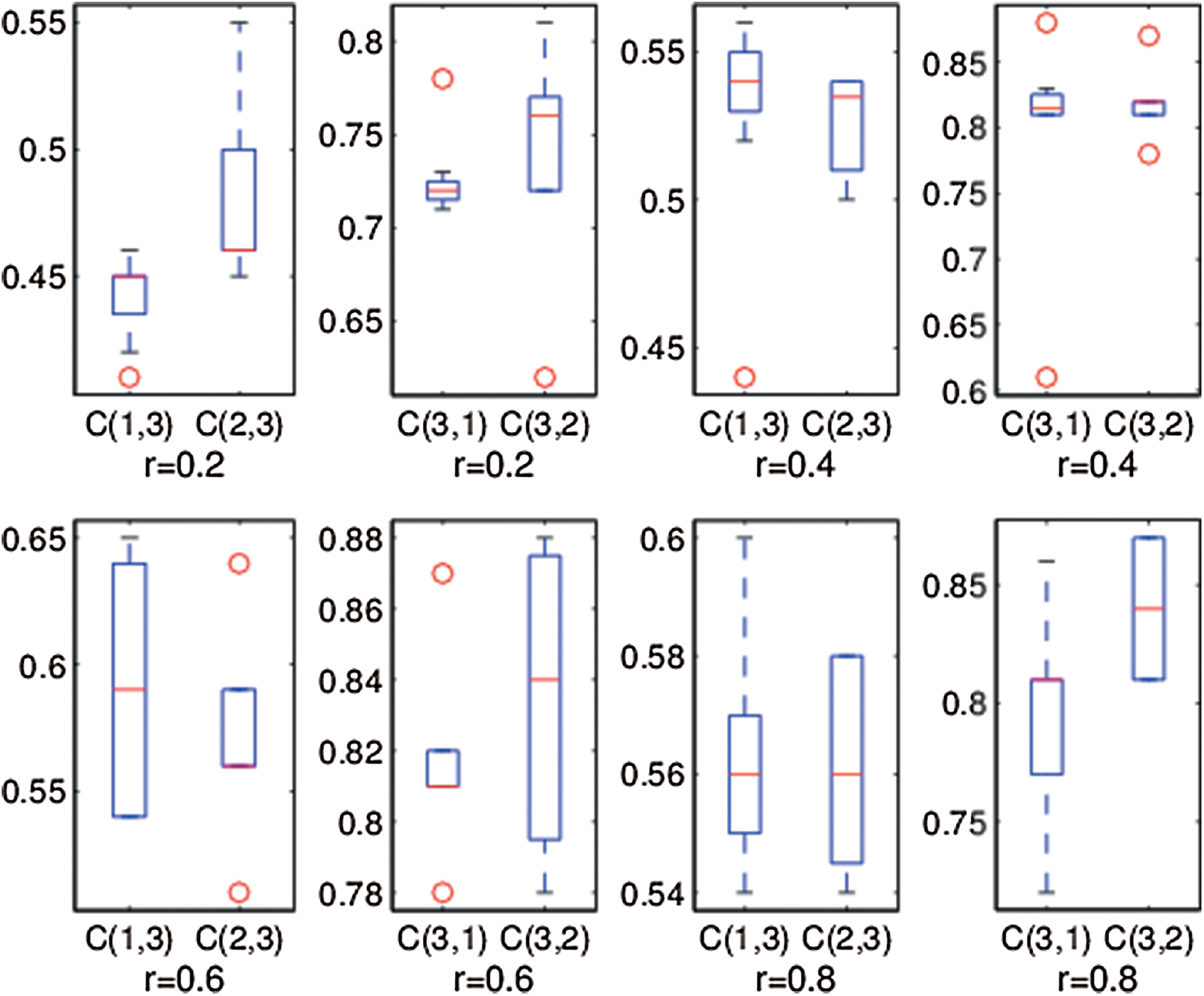
Figure 6: Comparison of C-measure obtained by algorithm s and m for Port2 in four values of parameter r, where  represents
  for
for 

Figure 7: Comparison of C-measure obtained by algorithm s and m for Port3 in four values of parameter r, where  represents
  for
for 

Figure 8: Comparison of C-measure obtained by algorithm i and j for Port4 in four values of parameter r, where  represents
  for
for 

Figure 9: Comparison of H-measure values obtained by three algorithms in different parameter r. The i-th row of the Figure representing the compared results of H-measure obtained by different algorithms for the i-th portfolio problem Porti in parameter r, 

Figure 10: Comparison of U-measure obtained by three algorithms in different parameter r. The i-th row of the Figure representing the compared results of U-measure obtained by three algorithms for the i-th portfolio problem Porti in parameter r, 
By comparing the portfolio efficient Pareto frontiers (Figs. 3 and 4) obtained by three compared algorithms DFEA, DCEA and DPEA in a typical run, we can easily know that our algorithm DPEA can obtain the true portfolio Pareto frontier more easily than algorithm DFEA and DCEA. Meanwhile, it can be observed from Fig. 5 to Fig. 8 that  for
for  in different parameter value r, which indicates that the Pareto solution set obtained by algorithm DPEA contains sufficient number of better solutions than that of the compared algorithms DFEA and DCEA, where
  and
and  are two Pareto solution sets obtained by the compared methods
  and
and  ,
,  presents the C-measure value obtained by algorithm
  and
and  , and the natural number 1, 2 and 3 present algorithms DFEA, DCEA and the proposed algorithm DPEA.
Moreover, comparing the Boxplot results in each row of Figs. 9 and 10, we can see that our algorithm DPEA produces bigger values of H-measure and much smaller values of U-measure than the compared algorithms DFEA and DCEA. These mean that the portfolio Pareto frontiers obtained by DPEA have better extension and uniform distribution than the two algorithms DFEA and DCEA, and the results also showed that the portfolio optimal solutions obtained by algorithm DPEA are superior to algorithm DFEA and DCEA. So, the given method DPEA is efficient in exploring and finding the portfolio optimal solutions for the biobjective portfolio problem (6).
In this paper, a hybrid ICA for solving biobjective portfolio problem and a new portfolio biobjective optimization model based on portfolio risk measure function and return measure function are given. In order to accelerate the convergence and produce quality Pareto portfolio fronts, a multi-colony levy crossover operator and a simple-colony moving operator with random perturbation are integrated into the proposed algorithm.
We utilized four portfolio benchmark problems to test the performance of the given algorithm DPEA according to three indicators C-measure, H-measure and U-measure. The results illustrate that algorithm DPEA can identify better portfolio optimal solutions and bring adequate diversity of the evolution population. That is to say, the portfolio efficient Pareto frontier obtained by DPEA is closer to the portfolio true Pareto front than the compared algorithms and its distribution is broader towards the boundary of the feasible search region. The results can not only help investors allocate and manage asset effectively but also provide better idea and method for solving other complicated constrained finance and economy problem.
Acknowledgement: The authors will gratefully acknowledge the anonymous reviewers for their valuable comments and suggestions.
Funding Statement: This work is supported by the Planning Fund for the Humanities and Social Sciences of the Ministry of Education (No. 18YJA790053).
Conflicts of Interest: The authors declare that they have no conflicts of interest to report regarding the present study.
1. P. N. Kolm, R. Tutuncu and F. J. Fabozzi. (2014). “60 years of portfolio optimization: Practical challenges and current trends,” European Journal of Operational Research, vol. 234, no. 2, pp. 356–371. [Google Scholar]
2. C. B. Kalayci, O. Ertenlice and M. A. Akbay. (2019). “A comprehensive review of deterministic models and applications for mean-variance portfolio optimization,” Expert Systems with Applications, vol. 125, pp. 345–368. [Google Scholar]
3. D. Kumar and K. K. Mishra. (2017). “Portfolio optimization using novel co-variance guided artificial bee colony algorithm,” Swarm and Evolutionary Computation, vol. 33, pp. 119–130. [Google Scholar]
4. M. Leal, D. Ponce and J. Puerto. (2020). “Portfolio problems with two levels decision-makers: Optimal portfolio selection with pricing decisions on transaction costs,” European Journal of Operational Research, vol. 284, no. 2, pp. 712–727. [Google Scholar]
5. H. Y. Zhang, G. L. Chen and X. W. Li. (2019). “Resource management in cloud computing with optimal pricing policies,” Computer Systems Science and Engineering, vol. 34, no. 4, pp. 249–254.
6. B. Wang, Y. Li and J. Watada. (2017). “Multi-period portfolio selection with dynamic risk/expected-return level under fuzzy random uncertainty,” Information Sciences, vol. 385-386, pp. 1–18.
7. S. S. Meghwani and M. Thakur. (2018). “Multiobjective heuristic algorithms for practical portfolio optimization and rebalancing with transaction cost,” Applied Soft Computing, vol. 67, pp. 865–894. [Google Scholar]
8. M. Masmoudi and F. B. Abdelaziz. (2018). “Portfolio selection problem: A review of deterministic and stochastic multiple objective programming models,” Annals of Operations Research, vol. 267, no. 1–2, pp. 335–352. [Google Scholar]
9. R. Ruiz-Torrubiano and A. Suárez. (2015). “A memetic algorithm for cardinality-constrained portfolio optimization with transaction costs,” Applied Soft Computing, vol. 36, pp. 125–142. [Google Scholar]
10. E. Baker, V. Bosetti and A. Salo. (2020). “Robust portfolio decision analysis: An application to the energy research and development portfolio problem,” European Journal of Operational Research, vol. 284, no. 3, pp. 1107–1120. [Google Scholar]
11. B. Li, Y. F. Sun, G. Aw and K. L. Teo. (2019). “Uncertain portfolio optimization problem under a minimax risk measure,” Applied Mathematical Modelling, vol. 76, pp. 274–281.
12. Z. F. Dai and F. Wang. (2019). “Sparse and robust mean-variance portfolio optimization problems,” Physica A: Statistical Mechanics and its Applications, vol. 523, pp. 1371–1378. [Google Scholar]
13. E. Fernandez, C. Gomez, G. Rivera and L. Cruz-Reyes. (2015). “Hybrid metaheuristic approach for handling many objectives and decisions on partial support in project portfolio optimization,” Information Science, vol. 315, pp. 102–122. [Google Scholar]
14. J. Li and J. P. Xu. (2013). “Multi-objective portfolio selection model with fuzzy random returns and a compromise approach-based genetic algorithm,” Information Science, vol. 220, pp. 507–521. [Google Scholar]
15. K. Lwin, R. Qu and G. Kendall. (2014). “A learning-guided multi-objective evolutionary algorithm for constrained portfolio optimization,” Applied Soft Computer, vol. 24, pp. 757–772. [Google Scholar]
16. K. P. Anagnostopoulos and G. A. Mamanis. (2010). “Portfolio optimization model with three objectives and discrete variables,” Computers & Operations Research, vol. 37, no. 7, pp. 1285–1297. [Google Scholar]
17. X. Deng and X. Q. Pan. (2018). “The research and comparison of multi-objective portfolio based on intuitionistic fuzzy optimization,” Computers & Industrial Engineering, vol. 124, pp. 411–421. [Google Scholar]
18. A. Ponsich, A. L. Jaimes and C. A. C. Coello. (2013). “A survey on multi-objective evolutionary algorithms for the solution of the portfolio optimization problem and other finance and economics applications,” IEEE Transactions Evolutionary Computer, vol. 17, no. 3, pp. 321–344. [Google Scholar]
19. R. B. Qi and G. G. Yen. (2017). “Hybrid bi-objective portfolio optimization with pre-selection strategy,” Information Sciences, vol. 417, pp. 401–419. [Google Scholar]
20. A. Mollajana, H. Memariana and B. Quintal. (2018). “Nonlinear rock-physics inversion using artificial neural network optimized by imperialist competitive algorithm,” Journal of Applied Geophysics, vol. 155, pp. 138–148. [Google Scholar]
21. C. A. Liu. (2016). “An imperialist competitive algorithm for solving dynamic nonlinear constrained optimization problems,” Journal of Intelligent & Fuzzy Systems, vol. 30, no. 2, pp. 759–772. [Google Scholar]
22. M. R. Maheri and M. Talezadeh. (2018). “An enhanced imperialist competitive algorithm for optimum design of skeletal structures,” Swarm and Evolutionary Computation, vol. 40, pp. 24–36. [Google Scholar]
23. A. Got, A. Moussaoui and D. Zouache. (2020). “A guided population archive whale optimization algorithm for solving multi-objective optimization problems,” Expert Systems with Applications, vol. 141, pp. 1–15. [Google Scholar]
24. J. Du, M. N. Yang and S. F. Yang. (2016). “Correlations and optimization of a heat exchanger with offset fins by genetic algorithm combining orthogonal design,” Applied Thermal Engineering, vol. 107, pp. 1091–1103. [Google Scholar]
25. A. S. M. Lacerda and L. S. Batista. (2019). “KDT-MOEA: A multi-objective optimization framework based on K-D trees,” Information Sciences, vol. 503, pp. 200–218. [Google Scholar]
26. W. Yue and Y. P. Wang. (2017). “A new fuzzy multi-objective higher order moment portfolio selection model for diversified portfolios,” Physica A: Statistical Mechanics and its Applications, vol. 465, pp. 124–140. [Google Scholar]
 | This work is licensed under a Creative Commons Attribution 4.0 International License, which permits unrestricted use, distribution, and reproduction in any medium, provided the original work is properly cited. |