Intelligent Automation & Soft Computing DOI:10.32604/iasc.2020.011723
Article

A Study of Unmanned Path Planning Based on a Double-Twin RBM-BP Deep Neural Network

Xuan Chen1,*, Zhiping Wan1 and Jiatong Wang2

1Zhejiang Industry Polytechnic College, Shaoxing, 312000, China
2Kunsan National University, Jeollabuk-do, 54150, Korea
*Corresponding Author: Xuan Chen. Email: chenxuan1979@sina.com
Received: 26 May 2020; Accepted: 27 August 2020

Abstract: Addressing the shortcomings of unmanned path planning, such as significant error and low precision, a path-planning algorithm based on the whale optimization algorithm (WOA)-optimized double-blinking restricted Boltzmann machine-back propagation (RBM-BP) deep neural network model is proposed. The model consists mainly of two twin RBMs and one BP neural network. One twin RBM is used for feature extraction of the unmanned path location, and the other RBM is used for the path similarity calculation. The model uses the WOA algorithm to optimize parameters, which reduces the number of training sessions, shortens the training time, and reduces the training errors of the neural network. In the MATLAB simulation experiment, the proposed algorithm is superior to several other neural network algorithms in terms of training errors. The comparison of the optimal path under the simulation of complex road conditions shows the superior performance of this algorithm. To further test the performance algorithm introduced in this paper, a flower bed, computer room and other actual scenarios were chosen to conduct path-planning experiments for unmanned paths. The results show that the proposed algorithm has obvious advantages in path selection, reducing the running time and improving the running efficiency. Therefore, it has definitive practical value in unmanned driving.

Keywords: Twin RBM-BP; WOA; path planning

1  Introduction

In recent years, driverless driving has been the focus of research in the automotive industry in various countries [1–3]. Yi et al. [4] proposed a design framework for unmanned driving trajectory planning based on real-time maneuvering decisions, dividing the trajectory space into homotopic regions, and linearizing the trajectory. The simulation experiment takes extreme conditions as the research object, which can effectively avoid accidents. Rajurkar et al. [5] proposed an optimal path-planning scheme for automatic vehicles based on a genetic algorithm to optimize the fuzzy controller. An automatic driving model based on neural networks has been proposed by NA. Neural networks have been widely used in many fields [6–9]. Li et al. [10] introduced deep learning into unmanned driving path planning and predicted the optimal path through a deep learning algorithm to guide the vehicle forward. Sallab et al. [11], Isele et al.[12], Pan et al. [13], Xia et al. [14], Xiong et al. [15] and others used deep reinforcement learning for unmanned driving and achieved good results. The problem with this type of research is that the number of iterations is vast. Generally, it can require more than 1000 sessions to obtain better training results, which increases the algorithm complexity. The training process also requires substantial data support.

For these problems, the paper has proposed a double twin RBP-BP deep learning neural network model based on WOA optimization. In this algorithm, a twin RBP model is used to process the feature map of the unmanned driving path, and another twin RBM model is used to process the path similarity. The WOA algorithm is used to optimize the twin RBM parameters in the deep learning network so that the deep learning neural network training error and the optimal parameters are obtained, which offers better prediction effects.

2  Related Knowledge

2.1 Restricted Boltzmann Machine

The restricted Boltzmann machine [16] is a neural network model based on statistical mechanics and an energy model. It uses energy to represent the stable state of the entire system. The smaller the energy usage is, the more stable the system is. Otherwise, it shows that the system is in a certain state of fluctuation and instability. It has the characteristics of a fast learning rate and strong learning ability. It is an important model in the field of deep learning. The structure is shown in Fig. 1.

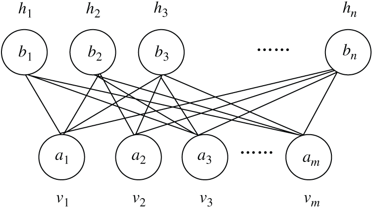
Figure 1: RBM structure

In Fig. 1 refers to the visible layer. Data samples are imported from the visible layer. refers to the hidden layer. It represents the characteristics of the extracted data. Suppose that the RBM network has visible units and hidden units. The vectors and refer to the status of the unit at the visible layer and the hidden layer. Suppose is the offset vector at the visible layer, and refers to the offset of the visible unit at the visible layer. Suppose is the offset vector at the hidden layer, and is the weighted matrix between the visible layer and the hidden layer. is the weight of the node and the node at the visible layer. The process of RBM training is to learn to obtain the parameter :

In Eq. (1), refers to the energy function of RBM. The network assigns a probability to each pair of visible and hidden vectors through the energy transfer function:

where Z is the partition function and its expression is:

Eq. (3) uses the following Eq. (4) to express the logarithmic gradient of weights:

where 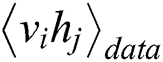is the expected data, and 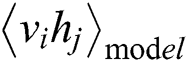is the expected model. Then, the RBM learning rules can be obtained as follows:

For data expectation, since there is no direct connection between RBM hidden layer units, an unbiased sample of data distribution can be quickly obtained. Suppose randomly given training images are , the probability of the binary state of the hidden layer unit being is:

For the same reason, the probability of the binary state of the visible layer unit is set to 1:

In summary, the main objective of RBM is to calculate . This is mainly obtained by calculating the maximum log likelihood of RBM on the learning set. The calculation Eq. (8) is as follows:

In order to obtain the optimal value of Eq. (8), it is calculated by the gradient ascent method [17]. The calculation process is as follows:

For the calculation of Eq. (9), the literature [18] is used to calculate the derivative, and the calculation process is as follows:

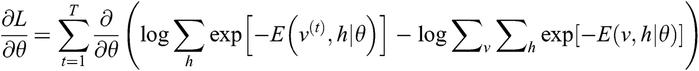
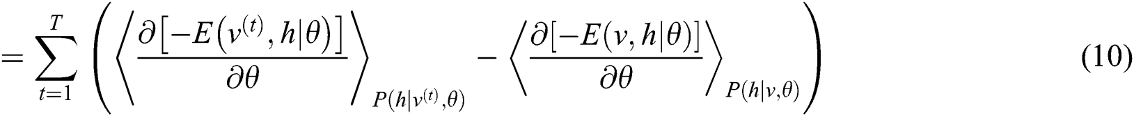
In Eq. (10), means the probability distribution of the hidden layer when the visible unit is set to uniform learning sample , means the joint distribution of visible units and hidden layer units. According to the two distributions, the offset number distribution of parameter is:

Eqs. (11)–(13) are RBM learning rules.

2.2 Whale Optimization Algorithm

The whale optimization algorithm [19] uses a set of search agents to determine the global optimal solution of the optimization problem. The search process for a given problem begins with a set of random solutions, and the candidate solutions are updated through optimization rules until the end conditions are met. The whale algorithm is divided into three stages: predation, bubble attack and food search.

(1) Surround predator

In the initial stage of the algorithm, humpback whales do not know where the food is; they all obtain the position information of the food through group cooperation. Other whale individuals will approach this position and gradually surround the food, so the following mathematical model is used:

In the Eq. (14), refers to the distance vector from the search agent to the target food, and refers to the current iteration times. and are coefficient vectors, is the local optimal solution, is the place vector, and and are expressed as follows:

In the Eq. (17), refers to the linearly decreasing vector from 2 to 0, and is a random number between 0 and 1.

(2) Bubble attack

In this stage, the humpback whale was used to attack the bubble, and the behavior of the whale preying and spitting out the bubble was designed by shrinking the surroundings and spirally updating the position to achieve the goal of local whale optimization.

1) Shrinking and surrounding principle

When , the individual whale approaches the best whale at its current location, and the larger is, the faster the pace of the whale.

2) Spiral update position

The individual humpback whale first calculates the distance from the current optimal whale and then swims in a spiral. When searching for food, the mathematical model of the spiral is:

In the Eq. (18), is the constant coefficient, and is a random vector between 0 and 1.

3) Food searching stage

Humpback whales obtain good results by controlling the vector. When , individual humpback whales have approached the position of the reference humpback whale, and the individual whale has updated its position toward the randomly selected humpback whale. The model is expressed as follows:

In the Eqs. (19) and (20), is a randomly obtained position vector of the reference humpback whale.

3  WOA-Optimized Dual Twin RBM-BP Neural Networks’ Unmanned Driving Path-Planning Algorithm

3.1 Theoretical Analysis of WOA Optimized Double-Twin RBM-BP

Because RBM parameter design is an extremely complicated task, RBM has no rules to follow during design, and it is difficult to ensure the optimization of the network. The parameter learning rate in the double-twin RBM-BP deep learning neural networks, the number of visible layers v, the number of hidden layers h, and the parameter set jointly determine the performance of the double-twin RBM-BP neural networks. Therefore, the parameter design complexity is more complicated than the traditional single RBM. Optimizing these six parameters reasonably is the key to the effectiveness of the model in this paper. Using genetic algorithms, particle swarm optimization and other biomimetic algorithms to optimize BP neural network parameters can improve its performance. Thus, this paper uses the more powerful WOA algorithm for parameter optimization of the twin RBM-BP deep learning neural networks. The parameters v, h, and a total of 12 sets of parameters in the twin RBM-BP are optimized by the WOA algorithm.

3.2 Training Model Based on the Double Twin RBM-BP Neural Network

The RBM-BP combines the advantages of RBM and BP and targets complex and high-dimensional network traffic data. We use RBM’s strong feature learning ability and unsupervised learning of high-dimensional data to remove redundant features and reduce data complexity. This can reduce the training complexity of the data and improve the recognition accuracy of the deep learning network. However, the RBM-BP networks require huge calculations and have shortcomings regarding the training sample library. In this paper, we will use double twin RBM-BP networks to achieve the use of a small number of layers to reduce the number of training sessions. The structure of twin RBM-BP is shown in Fig. 2.

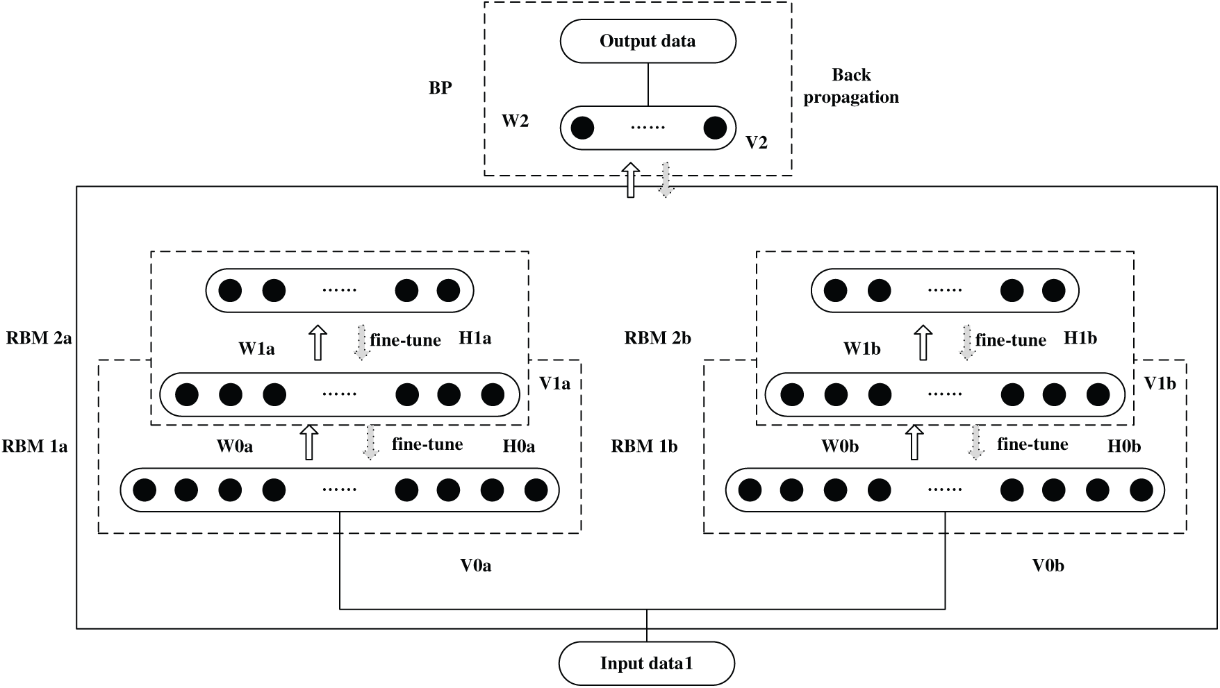
Figure 2: Double twin RBM-BP deep learning neural networks

3.3 WOA-Optimized RBM-BP Parameter

During the predation phase, refers to the location vector. In this paper, the variables that need to be optimized include the corresponding vectors of the parameter learning rate , number of visible layers v, number of hidden layers h and parameter set . Therefore, in Eq. (15) can be expressed as follows:

In the spiral phase, the optimization objective function involved in the calculation is the training error of the twin RBM deep learning neural networks, so it is expressed as:

Through optimization, the parameters v1,opt, h1,opt, 1,opt and 1,opt and v2,opt, h2,opt, 2,opt and 2,opt can be obtained. Apply the value of the two groups of the optimal parameters to the twin RBM deep learning neural networks to complete the optimization of the neural networks. Optimize two sets of parameters of twin RBM networks through WOA 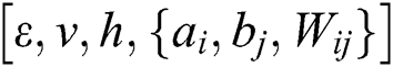to minimize the training errors.

3.4 Path Planning

After optimizing the RBM-BP deep learning neural network parameters through the WOA algorithm, the following two sets of RBM models and their corresponding learning rules can be obtained:

Eqs. (23) and (25) represent the model and learning rules of the first RBM in the twin RBM, which is mainly used for feature extraction of the input map data. After entering the map data matrix, neural networks are trained according to the obstacle area and non-obstacle area in the map. The training goal is to train with the shortest distance.

Eqs. (24) and (26) represent the model and learning rules of the second RBM in the twin RBM because there may be many different routes under the shortest distance between the starting point and the end point given at random. Therefore, it is necessary to analyze the similarity of these routes. In the route selection, routes with a small number of turns should be considered as much as possible, even if the number of turns is the same, as far as possible, and the angle of the turns is small. Therefore, the closeness between the optimal driving decision made by the twin RBM, and the actual target point is fed back to the neural network system as a feedback value.

3.5 Algorithm Process

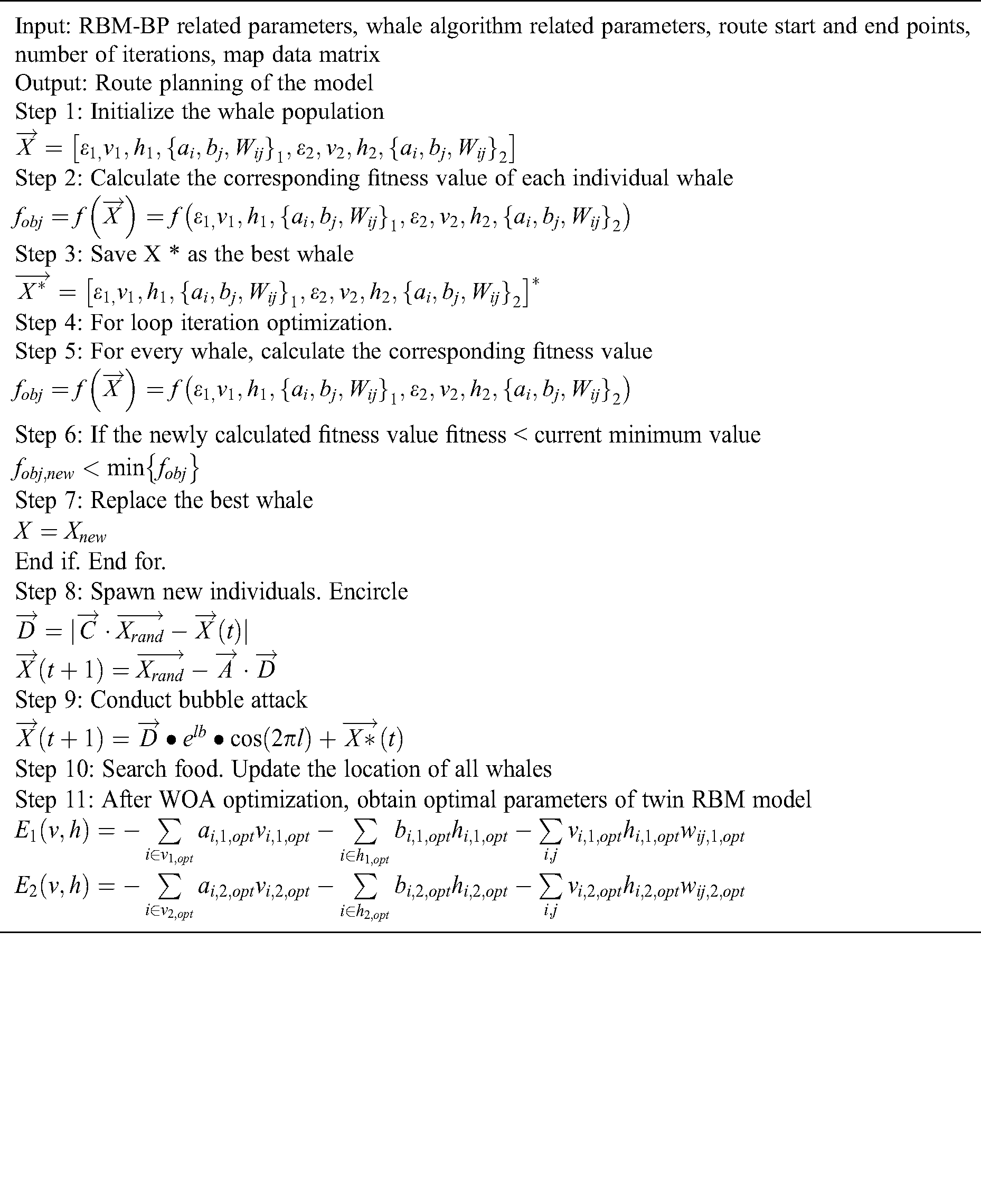
According to the process described above, the design process of the algorithm in this paper is shown in Tab. 1:

Table 1: Design process of the algorithm in this paper

4  Simulation Experiment

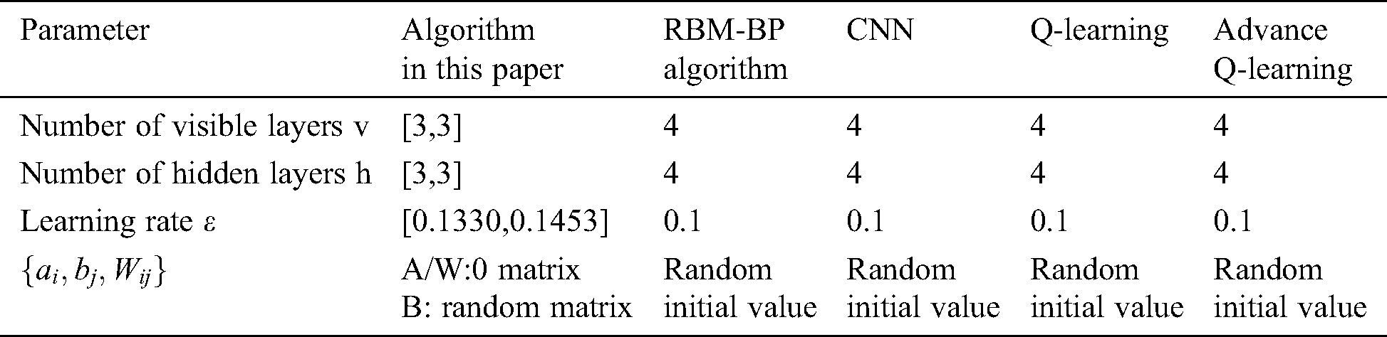
To further illustrate the route planning effect of the algorithm in this paper, the basic RBM-BP deep neural networks, CNN networks, Q-Learning network and the improved Q-Learning network are compared with the algorithm in this paper (as shown in Tab. 2). The content of the comparison includes the comparison of training error, optimal route length under complex road conditions and route planning effect. In the experiment part, the hardware platform is CPU i7-9700, memory 32GDDR3, Wins 10, simulation software MATLAB 2019. Take the unmanned driving smart car in Fig. 3 as the research object. The car consists of an FPGA chip of model zynq7020 (as shown in Fig. 4), a CCD camera, four infrared sensors, eight ultrasonic sensors, eight hall sensors (for detecting driving speed), four angle sensors (detection of steering), and an acceleration sensor. The circuit is shown in Fig. 5. To improve the effect of the simulation, the movement direction of the car is expressed as up, down, left, top left, bottom left, top right, bottom right, and eight directions. Set the motion space of the trolley to a two-dimensional plane and simulate the environment area as a 20 × 20 grid (as shown in Fig. 6).

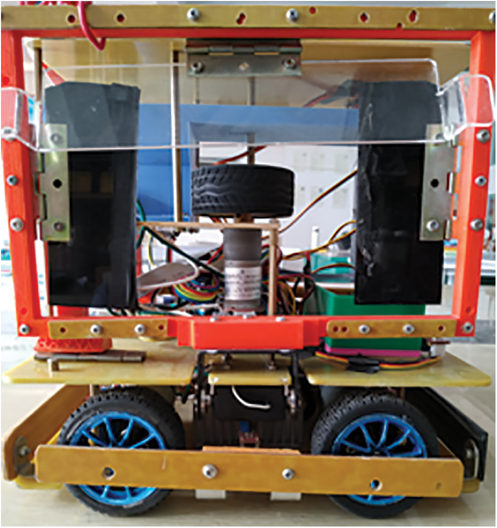
Figure 3: Unmanned driving intelligent car

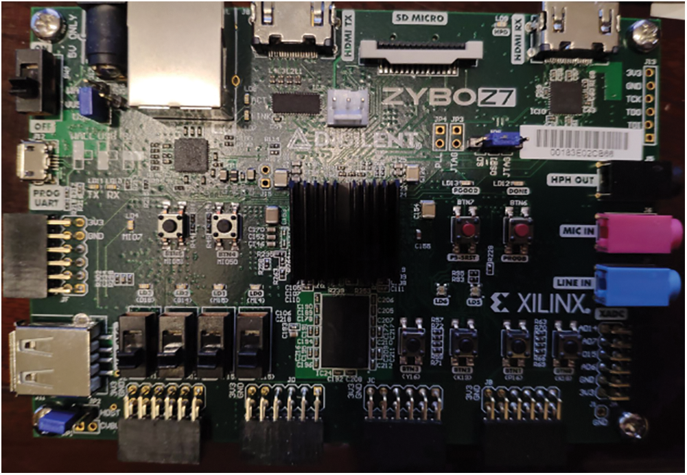
Figure 4: zynq7020 chip

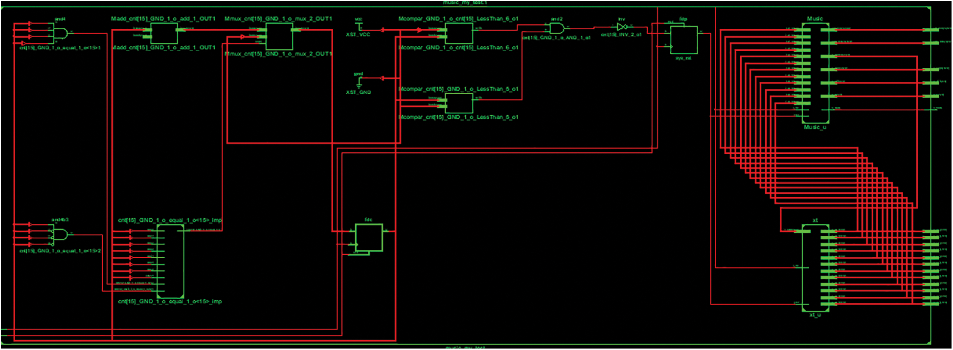
Figure 5: Circuit diagram

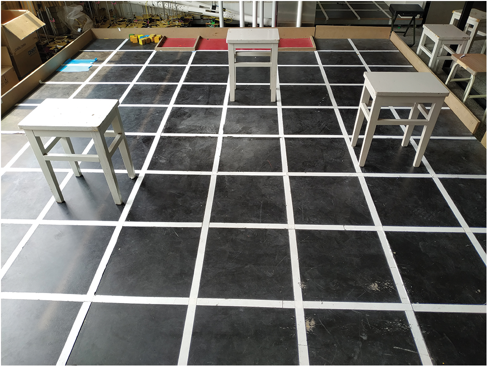
Figure 6: Simulated venue

Table 2: The main relevant parameters of the algorithm and comparison algorithm in this paper

4.1 Comparison of Optimization Indexes of Neural Networks under Different Algorithms

To verify the advantages of this algorithm in optimizing the parameters of double-stacked RBM-BP neural networks, this paper optimizes and contrasts the double-stacked RBM-BP neural networks using the genetic algorithm (GA), ant colony optimization (ACO), particle swarm optimization (PSO), and WOA algorithm. The source of the dataset is UCI wine quality [20]. Randomly select 1000 data points as the training dataset and select 100 data points from the remaining data points as the test dataset. All data of the training dataset and the test dataset are normalized between [−1,1]. Adopt the average variance mean square error (MSE) and mean absolute percentage error (MAPE). N is the total number of samples, yn is the predicted value, and tn is the actual value. The Eq is as follows:

Figs. 7–8. show the comparison of the five algorithms in the indexes MSE and MAPE. It is found from the training results of the algorithm in this paper are better than those of the other two algorithms.

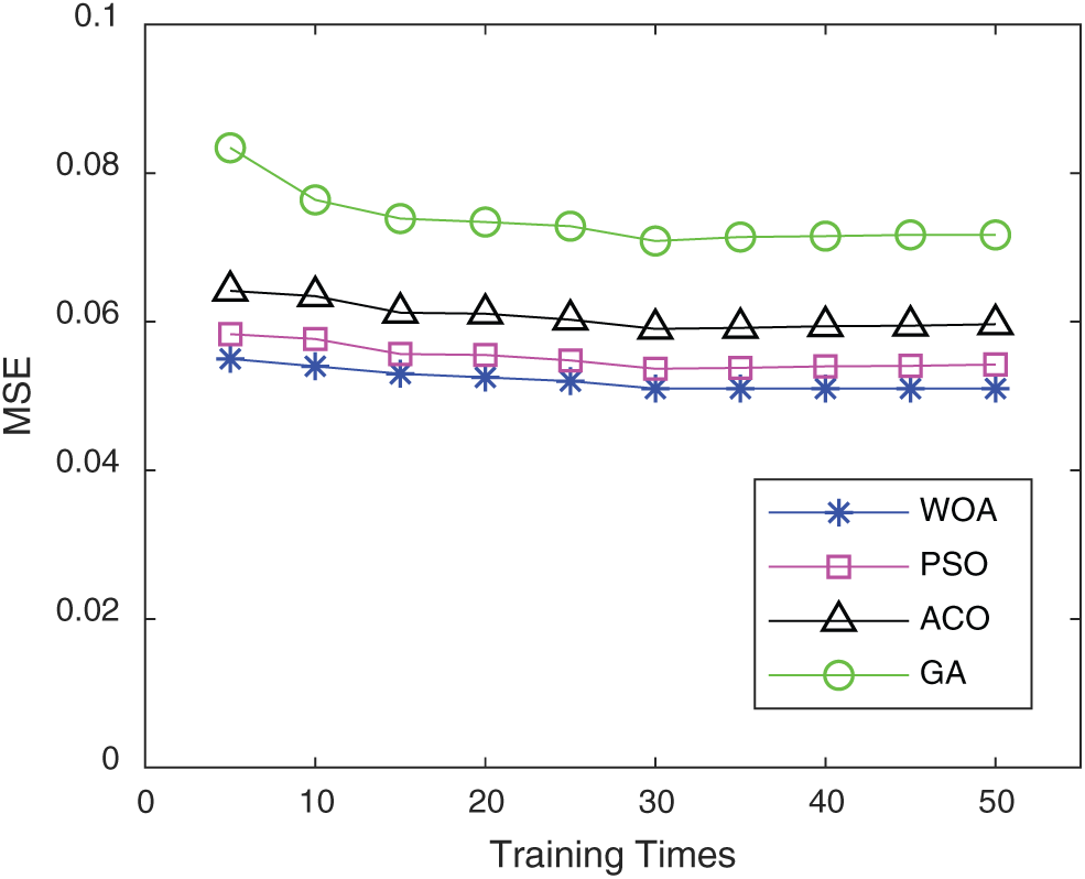
Figure 7: MSE comparison

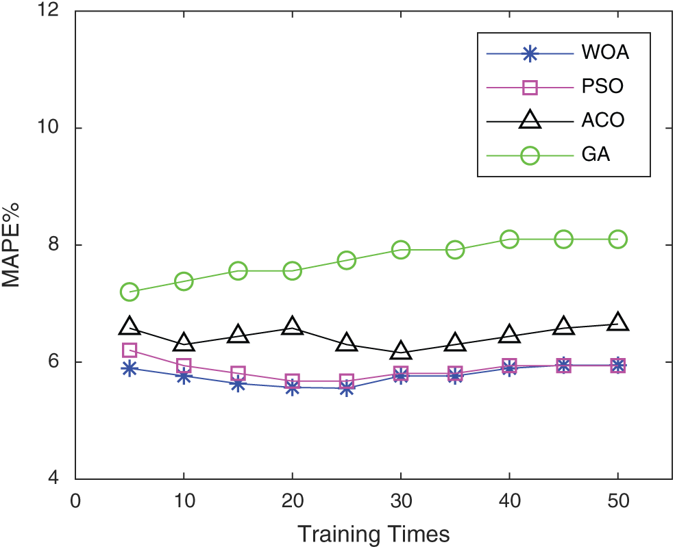
Figure 8: MAPE comparison

4.2 Comparison of Training Errors

Fig. 9 shows the comparison of the training errors under the five algorithms. It is found that as the iterations increase, the training errors of the five algorithms are reduced gradually. However, the error reduction rate of the algorithm in this paper is significantly better than that of the other four algorithms. When the number of iterations is approximately 175, the training error of the algorithm in this paper reaches convergence, while the basic RBM-BP only reaches the convergence value when the number of iterations reaches approximately 380, and CNN reaches convergence when the number of iterations is 396. Q-Learning reached convergence at 392 iterations, and improved Q-Learning reached convergence at 386 iterations. This shows that the algorithm in this paper uses twin RBM-BP to train the input data and WOA optimizes the neural network parameters to effectively reduce the number of training sessions, reduce the error rate, and achieve better training goals.

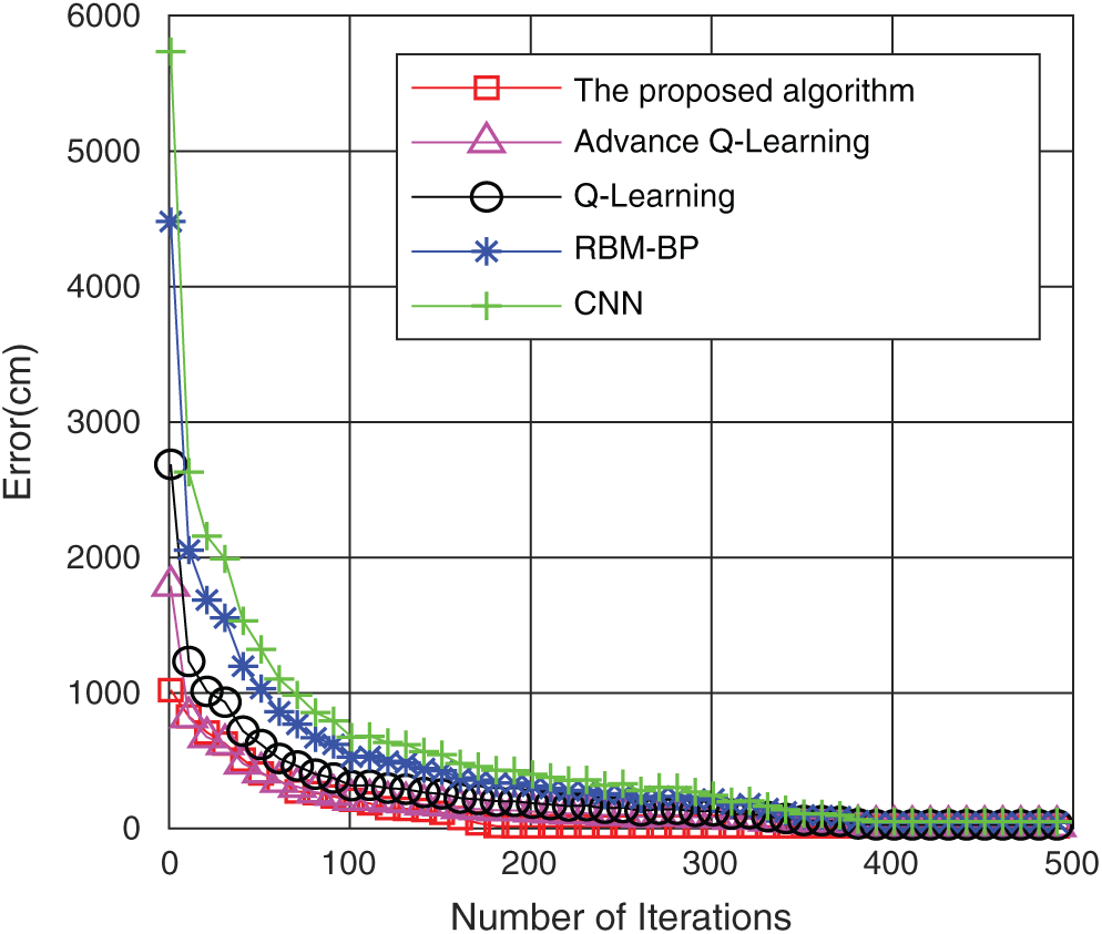
Figure 9: Comparison of the training errors of the five algorithms

4.3 Comparison of Path Lengths under Complex Road Conditions

Fig. 10 shows a schematic diagram of simulating a complex path, and Fig. 11 shows the path-planning effect of five algorithms in simulating complex road conditions. From the trajectory shown in the figure, the path length corresponding to the algorithm in this paper has obvious advantages. Compared with the RBM-BP, CNN networks, Q-Learning network and improved Q-Learning network are reduced by 16%, 28%, 16% and 8%, respectively. Fifty different sets of starting and ending points are randomly selected in the same scene, and the result of the average path is shown in Fig. 12. It can be found that the algorithm in this paper has certain advantages under the conditions of complex road conditions, mainly because the whale algorithm is optimized, so that the optimization effect of the parameters of the double-stacked RBM-BP networks is significantly improved. Therefore, it has a good planning effect under complex road conditions.

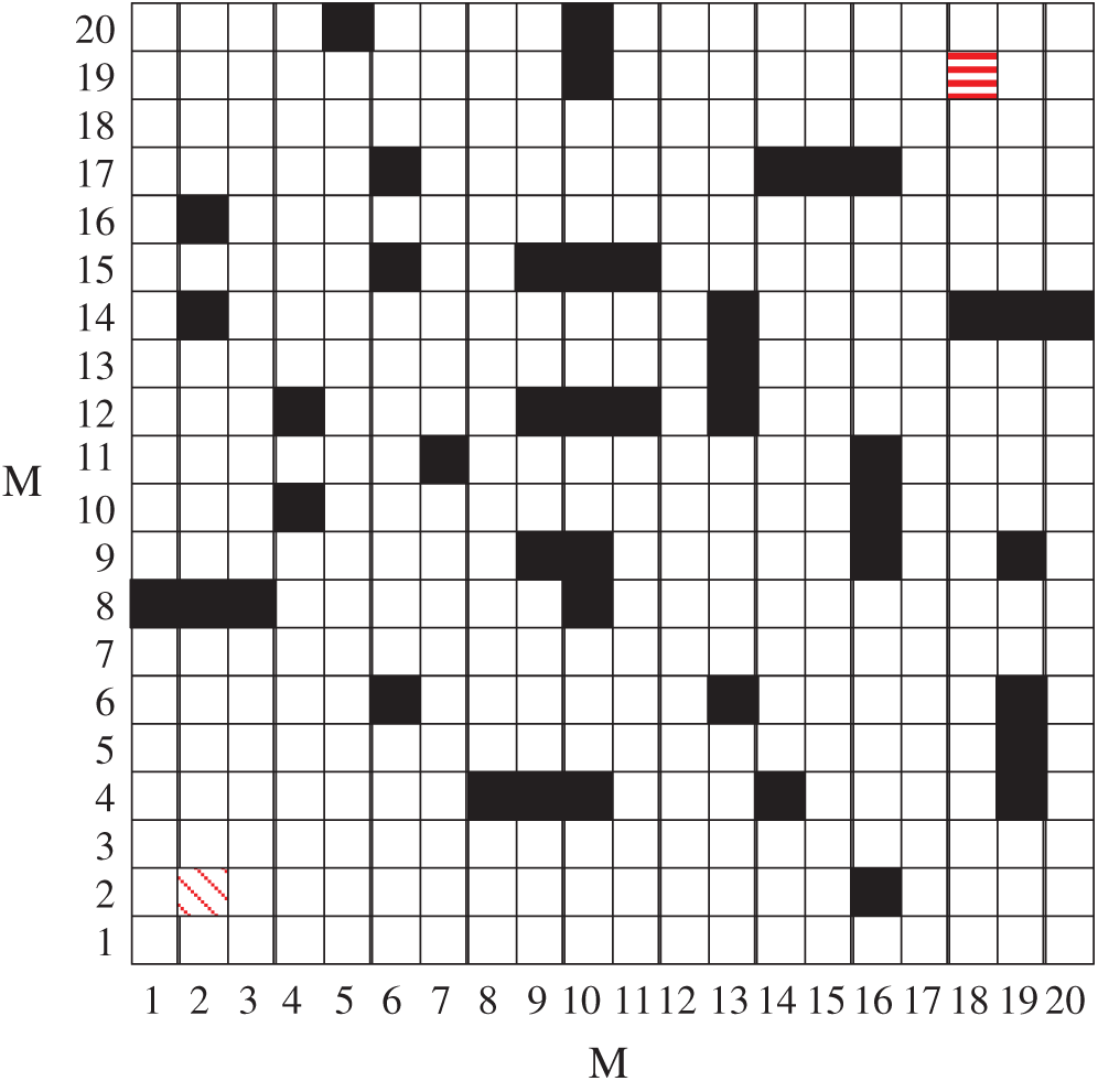
Figure 10: Schematic diagram of the complex path

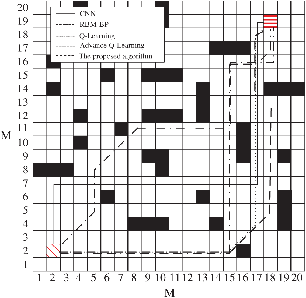
Figure 11: Schematic diagrams of five algorithm complex path trajectories

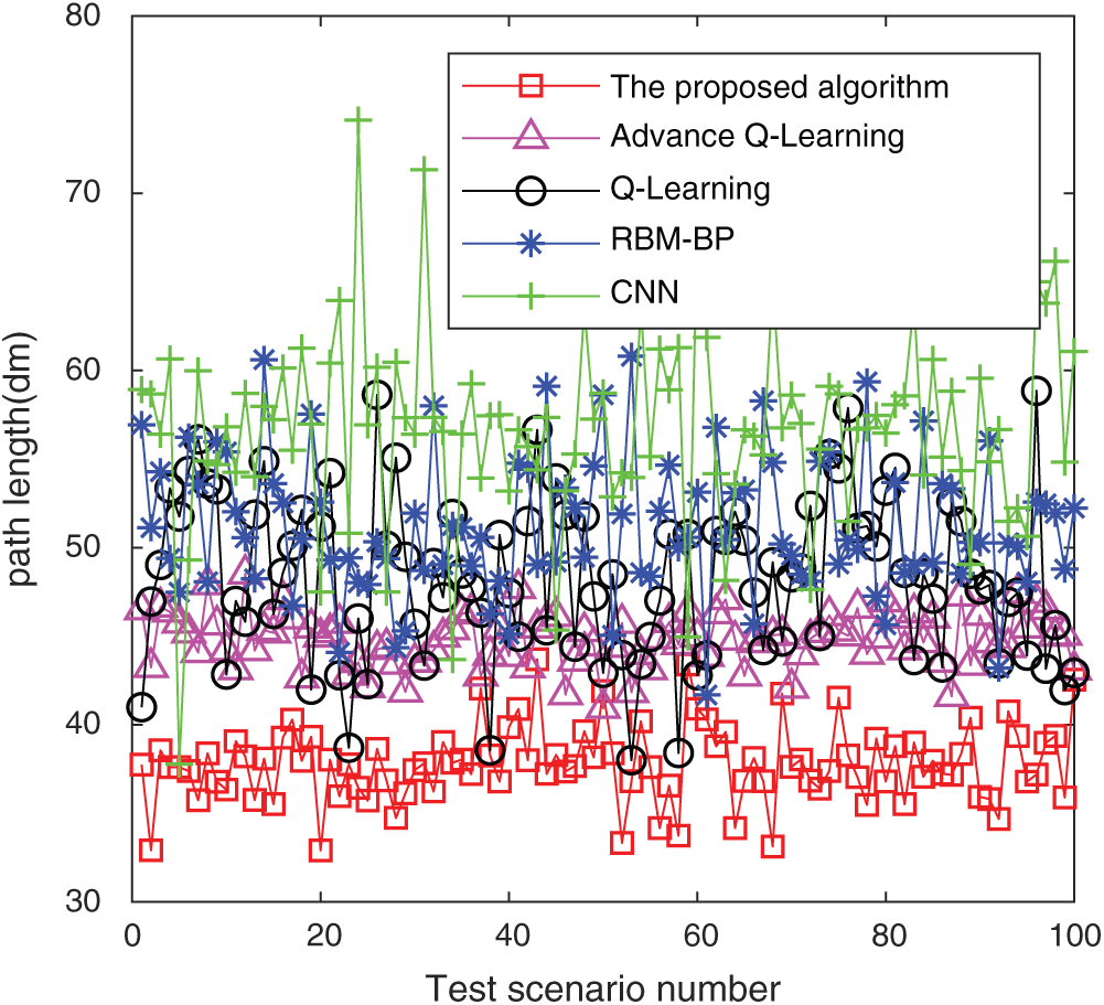
Figure 12: Comparison of 100 random starting and ending paths

4.4 Comparison of Path Lengths under Real Road Conditions

To further illustrate the effect of the algorithm in the real environment in this paper, the flower bed and the machine room were selected as comparative scenes, as shown in Figs. 13 and 14. The flower bed consists of 6 cylindrical flower ponds, which can imitate simple path conditions, and the machine room can imitate complex path conditions. The floor plans in the two scenes traveled under the five algorithms are shown in Figs. 15 and 16.

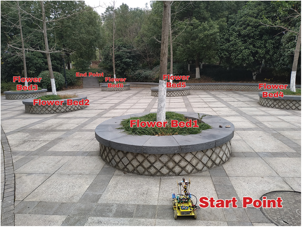
Figure 13: Garden scene

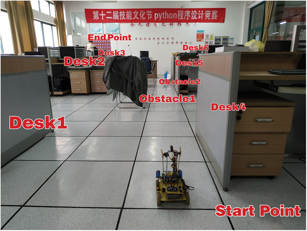
Figure 14: Computer room scene

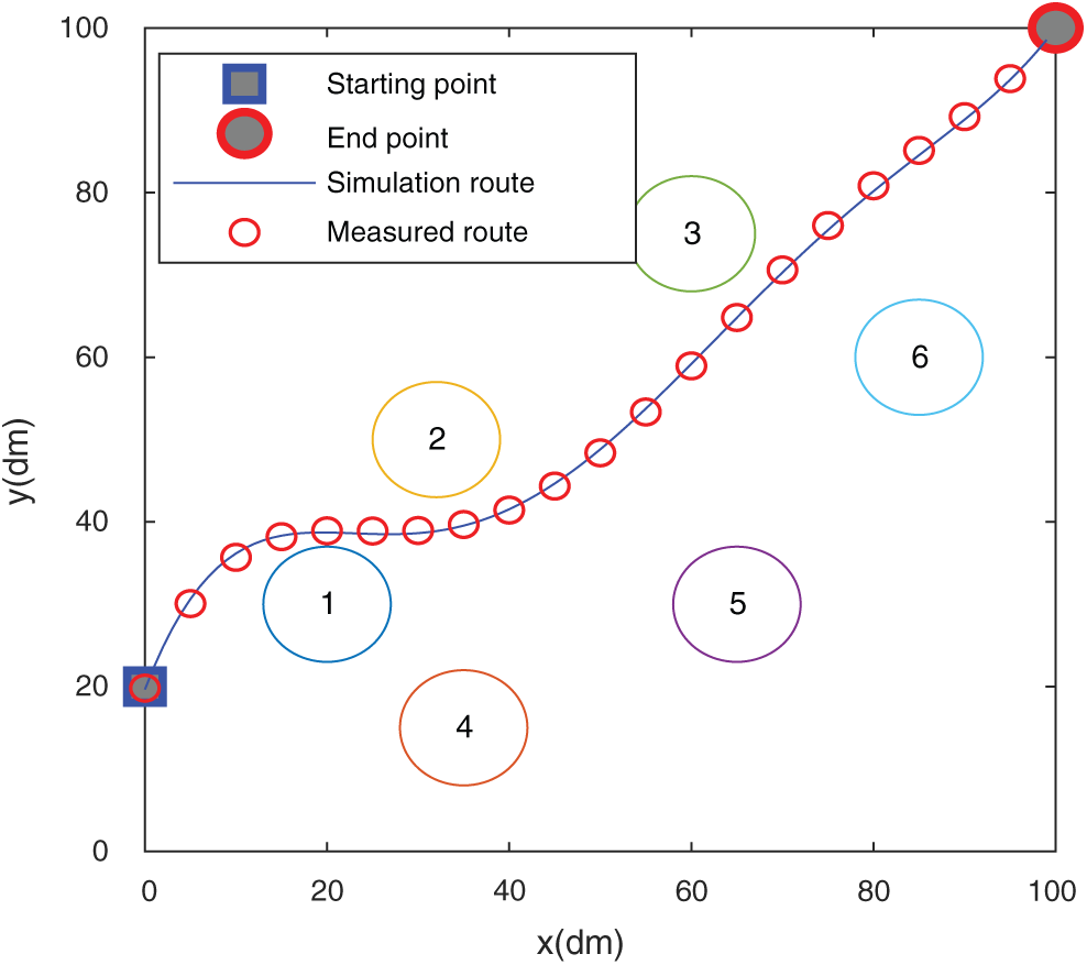
Figure 15: The trajectory in the flower bed

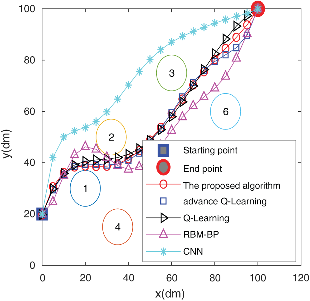
Figure 16: The trajectory in the flower bed

It is found from Figs. 15 and 17 that the simulated route of the algorithm in this paper almost matches the actual route traveled, which shows that the algorithm of this paper has a good result in path planning in actual scenarios. Figs. 16 and 18 show the comparison of the actual routes traveled by the five algorithms in the two scenarios. In Fig. 15, the algorithm of this paper circumvents the obstacle and goes directly to the end point. The trajectory does not show too much during the driving process. The curve is complete, and the RBM-BP route trajectory fluctuates greatly. The CNN curve has experienced two obstacles. The curve effect of Q-Learning and improved Q-Learning is slightly worse than that of the algorithm in this paper. The algorithm in Fig. 17 can circumvent obstacles and rush to the end in time, and the trajectory alters the least in the whole process, which shows that the planning effect of the algorithm in this paper is good. The path lengths of the CNN, RBM-BP and the improved Q-Learning are significantly greater than those of the algorithm in this paper. From the comparison of the results in the above figures, it has been shown that the algorithm in this paper has a better route planning effect in actual scenarios.

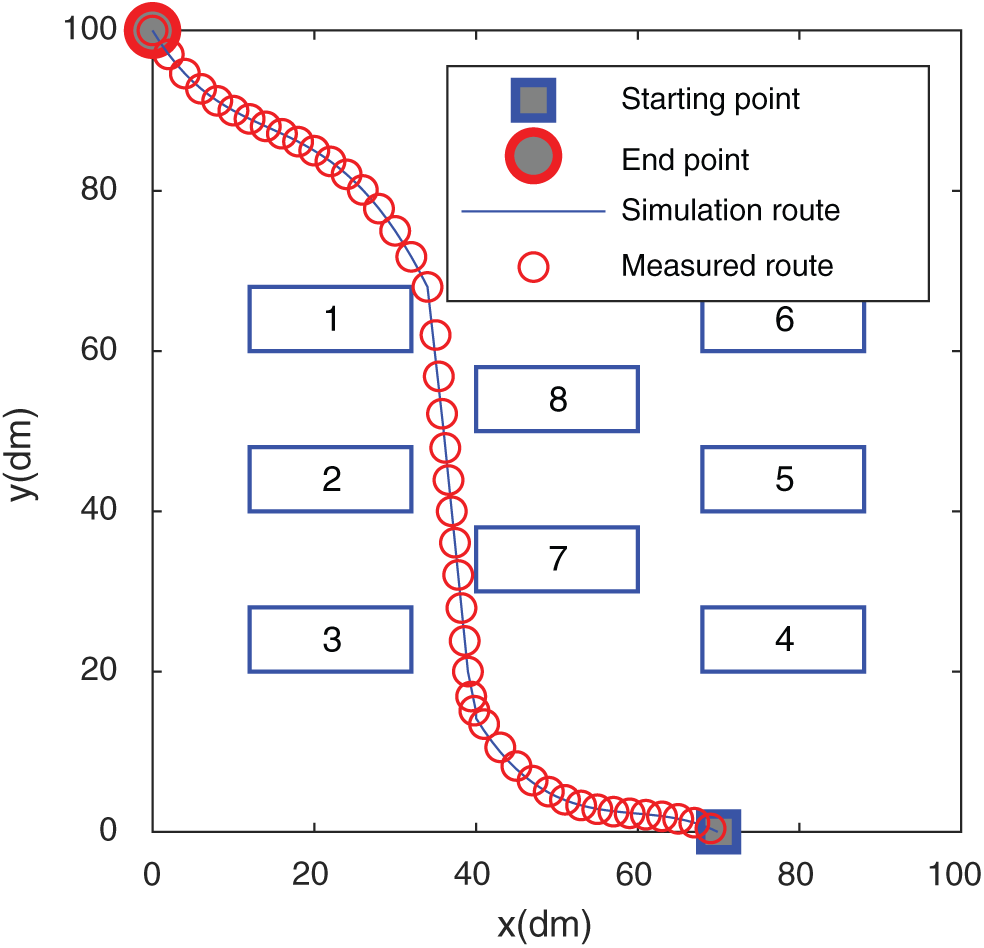
Figure 17: The trajectory in the computer room

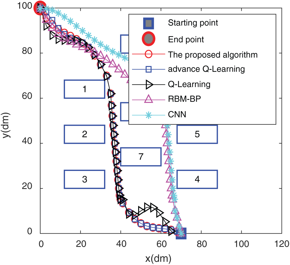
Figure 18: The trajectory in the computer room

5  Conclusion

In view of the problems of large error and long running time in the path planning of unmanned driving, the RBM-BP deep neural network algorithm based on double superposition is proposed. The algorithm calculates the characteristics and similarity of the path map through two superimposed RBMs. Then, the output feature vectors in the hidden layers of the two superimposed RBM networks are used as input feature vectors of BP neural networks for training and learning again. Finally, the whale algorithm is used to optimize multiple parameters, such as the number of visible layers, hidden layers and the learning rate, which reduces the training time and training errors. Simulation experiments show that the algorithm has a good path-planning result.

Funding Statement: This work is supported by the Public Welfare Technology Research Project of the Science and Technology Department of Zhejiang Province and Research on Key Technologies for Power Lithium-ion Battery Second Use in Energy Storage System (LGG19E070006).

Conflicts of Interest: The authors declare that they have no conflicts of interest to report regarding the present study.

This work is licensed under a Creative Commons Attribution 4.0 International License, which permits unrestricted use, distribution, and reproduction in any medium, provided the original work is properly cited.