A Computational Modeling on Flow Bifurcation and Energy Distribution through a Loosely Bent Rectangular Duct with Vortex Structure

1  Introduction

Curved channels (CC) are crucial in fluid transportation and heat transfer across various engineering and biological systems. In addition to engineering applications like heat exchangers and cooling ducts, fluid flow in CC mimics biological processes such as blood circulation and airflow through the trachea. Researchers have long focused on optimizing duct designs to reduce heat loss and improve performance. For ages, CC has been a centre of interest for many researchers and as a result, various shapes of ducts have been invented for smoothing the human lifestyle. Some references are given here to explain the importance of CC so that readers can get an obvious notion about it; these are Anisur et al. [1] and Sykes et al. [2] for curved rectangular duct (CRD), Zhang et al. [3] and Khan et al. [4] for curved square duct (CSD), Sheard et al. [5] and Miles et al. [6] for cylindrical duct, Sheard et al. [7] for circular tube, and so on.

One of the key aspects of fluid flow in a CC is the bifurcation, driven by centrifugal forces that generate secondary flows. Dean [8,9] first formulated the impact of curvature on fluid behavior, which has since been expanded by studies identifying bifurcation types like Hopf, pitchfork, and saddle-node bifurcations. However, a complete theoretical and experimental study on bifurcation was conducted by Benjamin [10,11], in which the theoretical study was made visualizing the existence of multiple bifurcation structures for a rotating cylinder and Taylor-vortex flows were studied experimentally where it was shown how 2-cell structure converted into a 4-cell structure with the increase of Reynolds number (Re). Bara et al. [12] performed experimental and numerical investigations to the obverse development of Dean vortices in a CSD and noticed multiple solutions.

The structural pattern of bifurcation with the association of other branches, stability of fluid convection, and the dynamic response rate of steady solution branches through a CSD is analyzed by Wang et al. [13]. Ghosh et al. [14] presented the steady boundary layer flow through a porous shrinking sheet in occupancy of heat and mass flux, in which the impact of heat and mass flux on temperature field and nanoparticle volume friction was revealed. Furthermore, they stated that in the first branch, the increment of fluid velocity is caused by the wall mass transfer; but the temperature and nanoparticle volume friction deteriorate for both the branches of solution. Chen et al. [15] performed the bifurcation of solution branches in a rectangular channel controlled by pressure gradient and aspect ratio (). Their study found two types of bifurcation; the first one was obtained in the range of and the other one in . Besides, the stable region, distribution limit, and bifurcation points are executed for the presence of both pressure gradient and aspect ratio. Adhikari et al. [16] presented the instability characteristics of fluid flow through a CSD of small curvature. Recently, Hasan et al. [17] investigated the effects of Coriolis force in bifurcation and flow transition through a tightly twisted square duct, where they explored time-dependent flow (TDF) in CSD imposing the rotational force (Coriolis force) both in the negative and positive directions and demonstrated various types of flow instabilities. The authors assigned that the flow changes from chaotic to periodic fluctuation followed by a steady-state solution later. However, the present paper adds new features not addressed in the above-mentioned studies, such as grid-point-specific velocity distribution in steady solution branches for various Dean numbers (Dn), which extends the understanding of steady-state solutions (SSs).

Unsteady flow (UF), depending on time, is another prominent fluid flow that can be observed to visualize the impact of centrifugal and buoyancy forces. Yanase et al. [18] first inspected the TDF through a CRD and next many more scholars were enticed to explore the nature of UF. The unsteadiness started with steady-state flow comprising a 2-vortex solution and ended with strong chaotic fluctuation with a 4- to 12-vortex solution. Mondal et al. [19] presented the results of TDF flow in a CSD heated in the outer wall and the fluid was driven by a comprehensive range of pressure gradients (). The unstable stream undergoes in the outline as steady-state→periodic→chaotic→periodic, where both steady and chaotic flow was composed of an asymmetric 2-vortex solution while periodic flow fluctuates between asymmetric 2- and 4-vortex solutions. Li et al. [20] conducted a combined experimental and numerical study on 3D flow development in a CRD with varying curvature. The flow fields were measured using Particle Image Velocimetry (PIV) and the numerical simulations were performed by solving the Reynolds Averaged Navier–Stokes (RANS) equations. Effects of curvature, Reynolds number, and aspect ratio on the Dean instability were discussed in that paper to accurately determine the core of secondary base vortices. The nonlinearity of unsteady solutions was examined by Dolon et al. [21] for a CRD flow of large aspect ratio and concluded that the newly created dean vortices have a significant impact on the variation of the flow pattern. In this study, Dolon et al. [21] completed spectral-based computational modeling on flow and heat transition for a CRD of strong curvature where various flow regimes were obtained and convective heat transfer (CHT) was substantially enhanced by centrifugal instability. Very recently, Mondal et al. [22] investigated a spectral-based numerical approach to study the nonlinear behavior of unsteady solutions with vortex structure in a bending square duct. Notwithstanding, none of the above-mentioned scholars analyzed grid-point-wise unsteady flow features and the current study fills up this gap.

Due to the presence of duct curvature, it is crucial to understand the thermal properties in a curved channel to mitigate the energy loss. For a large scale of Dn () and curvature (), Mondal et al. [19] applied a temperature gradient to the vertical sides of the duct to visualize the impact of curvature on UF and convective heat transfer (CHT). They observed that stability changes drastically when the curvature increases from 0.23 to 0.24, but when the flow is unstable, the secondary flow (SF) undergoes various flow impermanence such as periodic, multi-periodic, and chaotic enhancing the heat convection significantly. The inspection of this study explained that the 8-vortex chaotic flow enhanced the HC more than the 2-vortex steady-state solution. Experimental observation of conjugate HT of turbulent flow is performed by Guo et al. [23] in a bent square tube, where it was suggested the HT in a bent channel is 20% higher rather than in a straight channel. Recently, Adhikari et al. [24] performed a computational numerical study on laminar flow and thermal characteristics through a strongly bent square duct. By analyzing the Nusselt number (Nu), they showed that chaotic flow enhances CHT in the flow substantially. Very recently, Hussen et al. [25] investigated a spectral-based numerical approach to study the nonlinear behavior of unsteady solutions with vortex structure and heat transfer characteristics in a bending square duct. However, a correlation between heating-induced buoyancy force and centrifugal instability is still absent in literature to investigate the baffling flow behavior and energy distribution in a bending rectangular flow, which is one of the objectives of the present study. Despite significant progress, there are still gaps in the literature. For example, grid-point-specific velocity analysis has rarely been used to explore local flow behaviors in detail. Additionally, while chaotic flow regimes have been identified, the relationship between buoyancy-induced heating and centrifugal instability remains underexplored. This study aims to fill up these gaps by analyzing the branching structure of solutions across a wide range of Dn’s, focusing on vortex formation and chaotic flow patterns.

The main objective of this work is to investigate nonlinear behavior and CHT through a bent rectangular duct. Using a spectral-based numerical method, we examine laminar flow patterns under varying Dean numbers and quantify energy distribution. The study considers a duct where the bottom and outer walls are heated, while the inner and upper walls are kept at room temperature. This setup allows for a deeper understanding of how curvature, flow regime, and wall heating interact enhancing heat transfer in the flow.

2  Mathematical Model and Formulation

Assuming a fully developed 2D flow of viscous incompressible fluid passes through a CRD whose height and width are 2h and 2d, respectively. The cross-sectional view with corresponding notations is displayed in Fig. 1, where C, O, and L represent the center of the duct, the center of the curvature, and the radius of the curvature of the cross-section, respectively. The axis- directs the horizontal path while the axis- and are chosen in the vertical and axial directions, respectively.

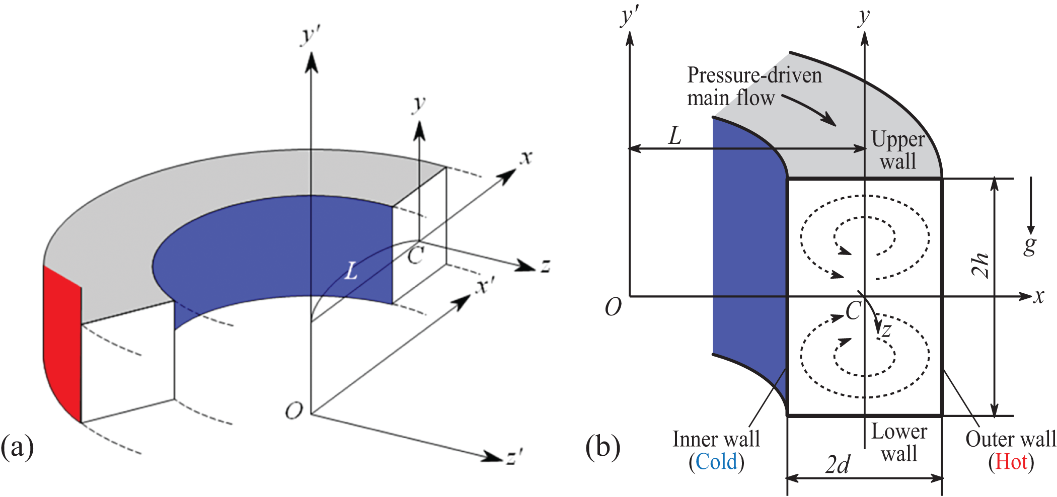
Figure 1: (a) Coordinate system of the bending duct; (b) Cross-sectional view

Let be the velocity components in the -directions, respectively. The equation of mass conservation, momentum, and energy equation can be written as follows:

Mass conservation equation:

(1)

Momentum equation:

(2)

(3)

(4)

Energy equation:

(5)

where

Employing the radius of curvature (L), and the width of the cross-section (d), the dimensional cylindrical coordinates can be transformed into non-dimensional rectangular coordinates under the transformation:

The sectional stream function is introduced as

(6)

where, . Therefore, the obtained non-dimensional equations for and are expressed as

(7)

(8)

(9)

where

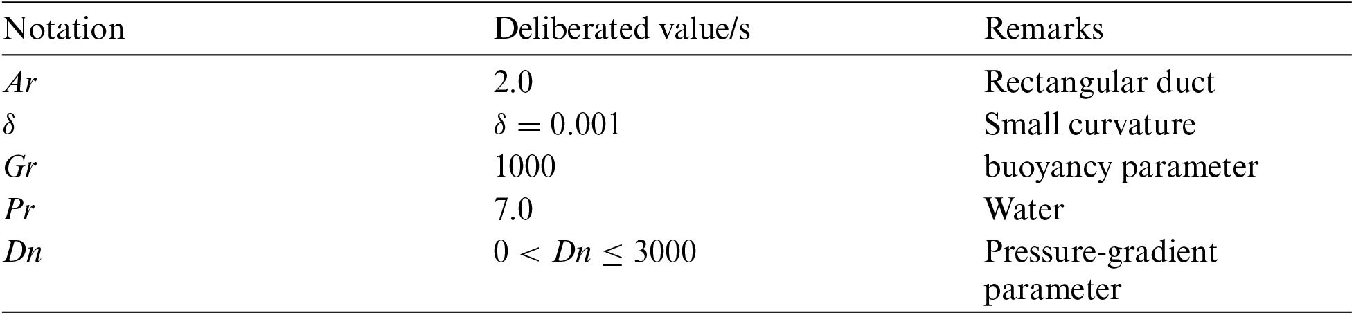
The dimensionless parameters which are used in the equations from (7) to (9) are the Dean number, ; the Grashof number, ; and the Prandtl number, . The rigid boundary conditions for and are

(10)

and the thermal boundary conditions for are

(11)

3  Numerical Calculations

3.1 Method of Numerical Execution

As this investigation is based on numerical approximation, the Spectral method is considered a good approach to solving the Eqs. (7)–(9) (Gottlieb et al. [26]). Here, in a series, the variables will be expanded including Chebyshev polynomials, i.e., and are the expanded functions can be narrated as

(12)

where represents the Chebyshev polynomial of order. What is more, and are applied to expand and as

(13)

The collocation points are taken as

(14)

Steady solutions are obtained by the Newton-Raphson iteration method as

(15)

where is the iteration number. The assurance of convergence is instituted as small as possible for ( < ) defined as

(16)

At last, to get the solution of UF, Crank-Nicolson (C-N formula) and Adams-Bashforth (A-B method) strategies are applied to the Eqs. (7)–(9).

3.2 Resistance Coefficient (R-C)

The definition of flow resistance coefficient (λ) is expressed as

(17)

The mean axial velocity is enumerated by

(18)

Since is related to the mean non-dimensional axial velocity as

(19)

3.3 The Nusselt Number

According to Mondal et al. [27], the Nusselt number to find out the heat transfer in steady solution branches can be expressed as

(20)

where are denoted the Nusselt number for cooled and heated sidewalls, respectively. On the contrary, for unsteady solutions, it is defined as

(21)

3.4 Numerical Accuracy

Here, the percentage errors of our present study will be justified while executing numerical values by the grid efficiency method since the effectiveness of the algorithm for the governing equations can be supported by this significant method. The necessity of grid accuracy was realized by Wang et al. [28] when they visualized the variation of bifurcation structure with the variation of grid points. Though Dolon et al. [21] investigated the accuracy of the numerical algorithm, the authors did not find any relative percentage error. In the present study, the grid efficiency is represented by relative percentage error for both R-C () and axial velocity () using the fixed value of , and aspect ratio Ar = 2.0 for various grid sizes as 14 × 28, 16 × 32, 18 × 36, 20 × 40, 22 × 44, 24 × 48, 26 × 52. Our obtained percentage errors for both and are presented in Table 1 and are shown graphically in Fig. 2. The formula that is used to find out the percentage error is

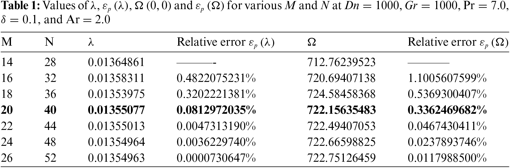
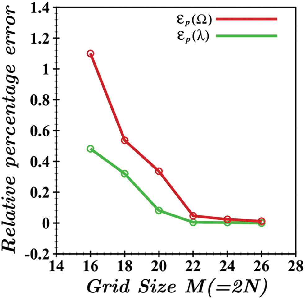
Figure 2: Relative percentage error regarding various grid sizes for and

It is seen from Table 1 that and changes to 0.4822075231% and 1.1005607599% respectively when the grid points are changed from to . Both and are reduced monotonically as the grid points are increased. For 20 × 40 when these grid sizes are altered from 18 × 36, then and are figured out as 0.0812972035% and 0.3362469682% consequently. With the increment of grid sizes, more accuracy is obtained which is noticed in Fig. 2. Considering all these aspects, M = 20, and N = 40 grid sizes are used in our present study to execute the numerical solutions because substantial accuracy can be obtained using this grid size.

3.5 Experimental vs. Numerical Outcomes

This section provides a detailed validation of our numerical outcomes by comparing them with experimental results to confirm the accuracy of the secondary flow structures and temperature distribution. The experimental vortex structures were observed by Chandratilleke [29,30] and Sugiyama et al. [31] for a curved rectangular duct (CRD) with an aspect ratio of Ar = 2.0. As displayed in Fig. 3, the secondary flow structures on the right are the current numerical results while the left displays the experimental results by Chandratilleke [29] (Fig. 3a) and Sugiyama et al. [31] (Fig. 3b). Furthermore, on the left in Fig. 3c,d. Chandratilleke [29] found the temperature field of outside heated CRD by using CFD tools. Chandratilleke [29,30] focused on the secondary flow characteristics and convective heat transfer in a CRD with external heating, revealing the formation of secondary vortices and their impact on heat transfer efficiency. Sugiyama et al. [31] visualized the secondary flow in curved rectangular channels providing insights into the flow patterns and vortex structures.

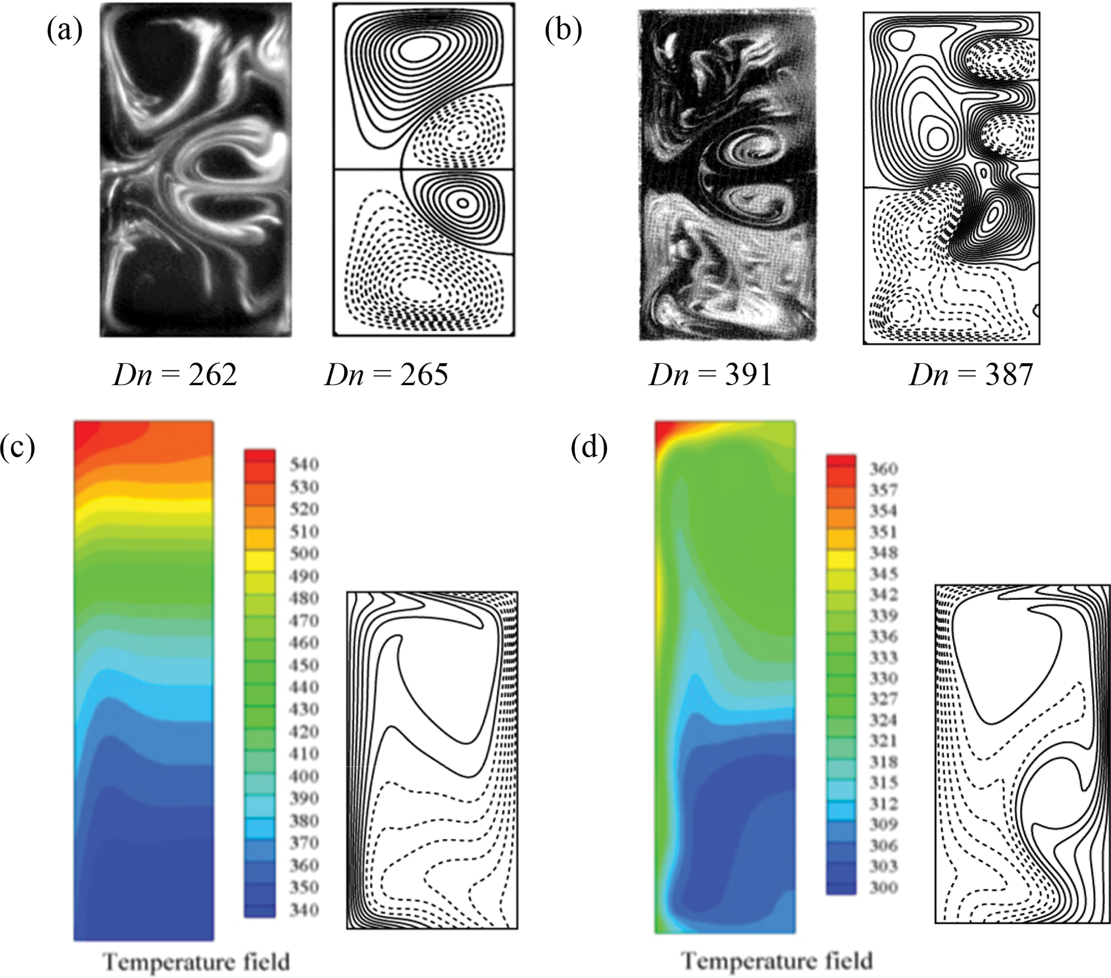
Figure 3: Comparison of numerical data with the experimental outcomes for curved rectangular duct flow. Left: Experimental contour (a) Chandratilleke [29,30]; (b) Sugiyama et al. [31], (c, d) Chandratilleke et al. [32] and right: (a–d) numerical contour by the authors

Using CFD tools, Chandratilleke et al. [32] analyzed the temperature field in an externally heated CRD highlighting the thermal behavior and heat transfer mechanisms. Our numerical simulations, conducted using a spectral-based numerical approach, accurately captured the secondary flow patterns and vortex structures observed in the experiments. The comparison of numerical and experimental results, shown in Fig. 3, where the left side displays the experimental results and the right side shows the numerical results, confirms the validity of our numerical approach. The temperature distribution obtained from the numerical simulations also showed a high degree of agreement with the experimental CFD results by Chandratilleke et al. [32] demonstrating the reliability of the numerical method in predicting thermal behavior.

4  Results

Considering the following parametric values with particular notations, an extensive discussion is made about the structure of bifurcation, the oscillatory flow phenomena, heat generation, distribution from the wall to the fluid, vortex formation, grid point-wise velocity transformation, and so on.

4.1 Branching Structure of Steady Solutions

After a comprehensive exploration, we have procured four branches of steady solutions (SS) in the fluid while flowing through the RCD. The bifurcation diagram in Fig. 4a shows the relationship between the Dean number and the flow resistance coefficient (). The diagram reveals multiple branches of steady solutions, each corresponding to different flow patterns. The first branch, which spans the entire range of the Dean numbers, represents the primary flow structure with a single vortex. The second, third, and fourth branches correspond to more complex flow patterns with multiple vortices. These branches exhibit various bifurcation points, where the flow transitions from one steady-state solution to another. The illustrated figure is so perplexing and that’s why we have drawn an enlargement of the entangled part for a larger Dn in Fig. 4b.

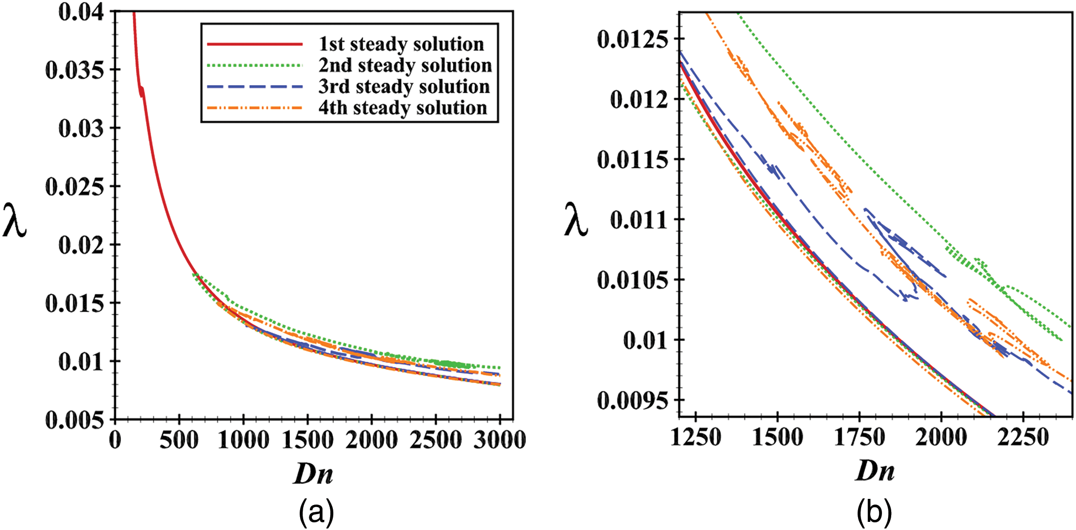
Figure 4: (a) Combined structure of steady solution branches, (b) Enlargement of Fig. 4a for

The branching structure of steady solutions involves understanding the bifurcation phenomena in fluid dynamics. Bifurcation occurs when a small change in the system’s parameters, such as the Dean number, causes a sudden qualitative change in its behavior. In curved ducts, the centrifugal force induced by the curvature leads to the formation of secondary flows, which can bifurcate into multiple steady-state solutions. These solutions represent different flow patterns, characterized by the number and arrangement of vortices. The stability of these solutions depends on the balance between the centrifugal force, pressure gradient, and thermal effects. As the Dean number increases, the flow transitions through various bifurcation points, leading to the complex branching structure observed in the steady solutions.

The 1st SS branch ccupying the whole range of Dn is depicted in Fig. 5a for . This branch starts at point a (Dn ≈ 0) and prolongs with the rising and decreasing λ up to point b(). It then turns back to point c and the branch finally reaches point d without further turning. Fig. 5b is the enlargement of Fig. 5a at points b and c which indicates very smooth turning. The axial velocity distribution (AVD), secondary flow pattern (SFP), and energy profiles at various Dn in this branch are shown in Fig. 5e,f. At , the axial velocity exists in the central line while turning to the left, i.e., near the outer boundary of the duct with high velocity at which is justified by Fig. 5c,d, respectively because frequencies of path lines at are higher than that of . It is transparent that the velocity, however, with the growth of Dn, increases on the boundary, and the maximum velocity is marked up at . The first branch consists of a single-vortex to a 3-vortex solution which starts with a single-vortex solution with low pressure and ends as an asymmetric 2-vortex with high pressure. The single vortex remains up to and then a new vortex is created on the outer wall of the duct because of heating-induced buoyancy force. The 2nd SS branch between and is illustrated in Fig. 6a. Though the lower part of the branch looks quite simple starting at point a () to point b , many complexities can be noticed with some smooth and sharp turnings between the ranges and (see Fig. 6c,d).

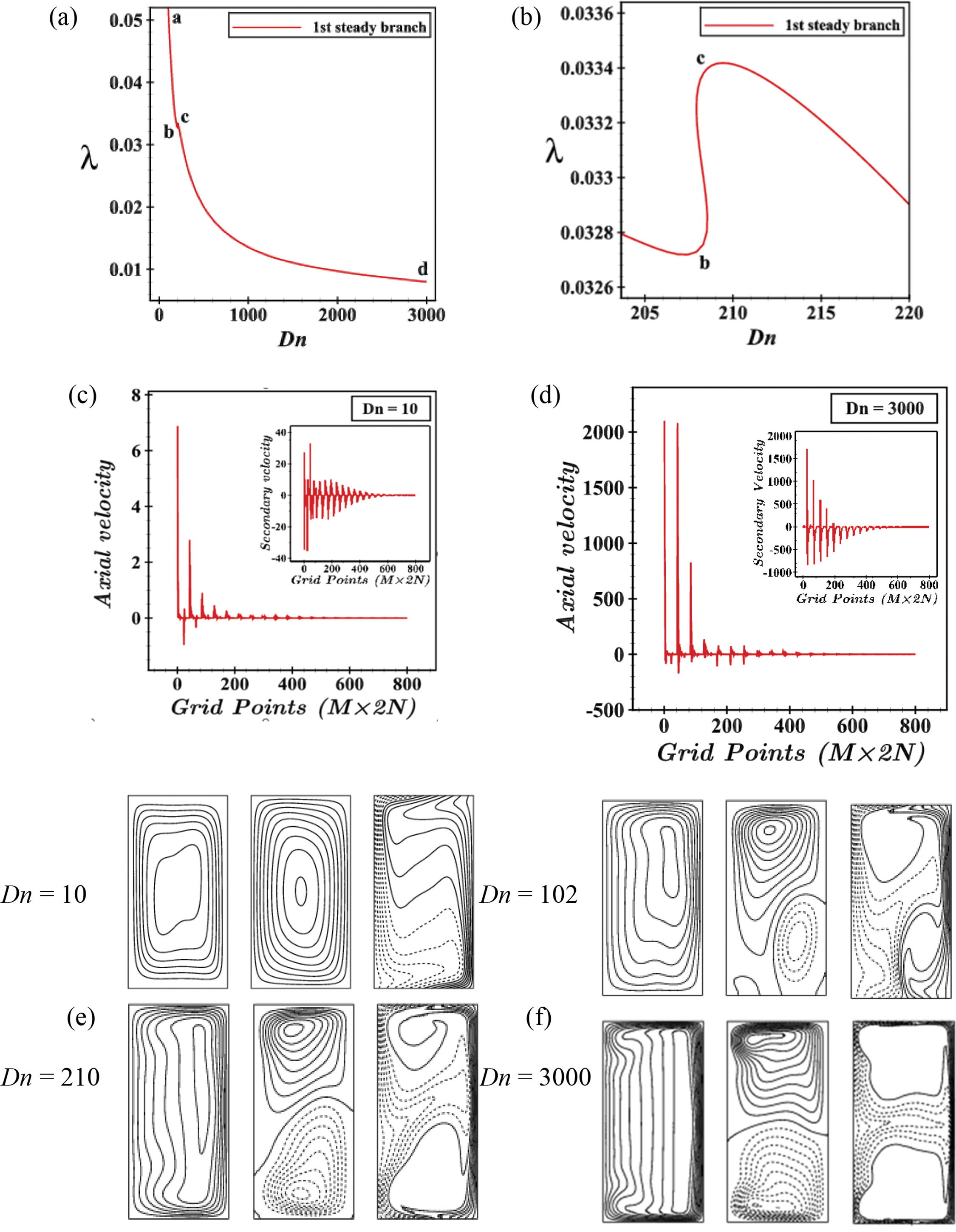
Figure 5: (a) 1st steady solution branch; (b) Enlargement of (a); (c, d) are axial velocity and secondary flow pattern for Dn = 10 and 3000; (e, f) Contours of axial flow (Ω), secondary flow (Ψ) and temperature profiles (τ) for various values of Dn

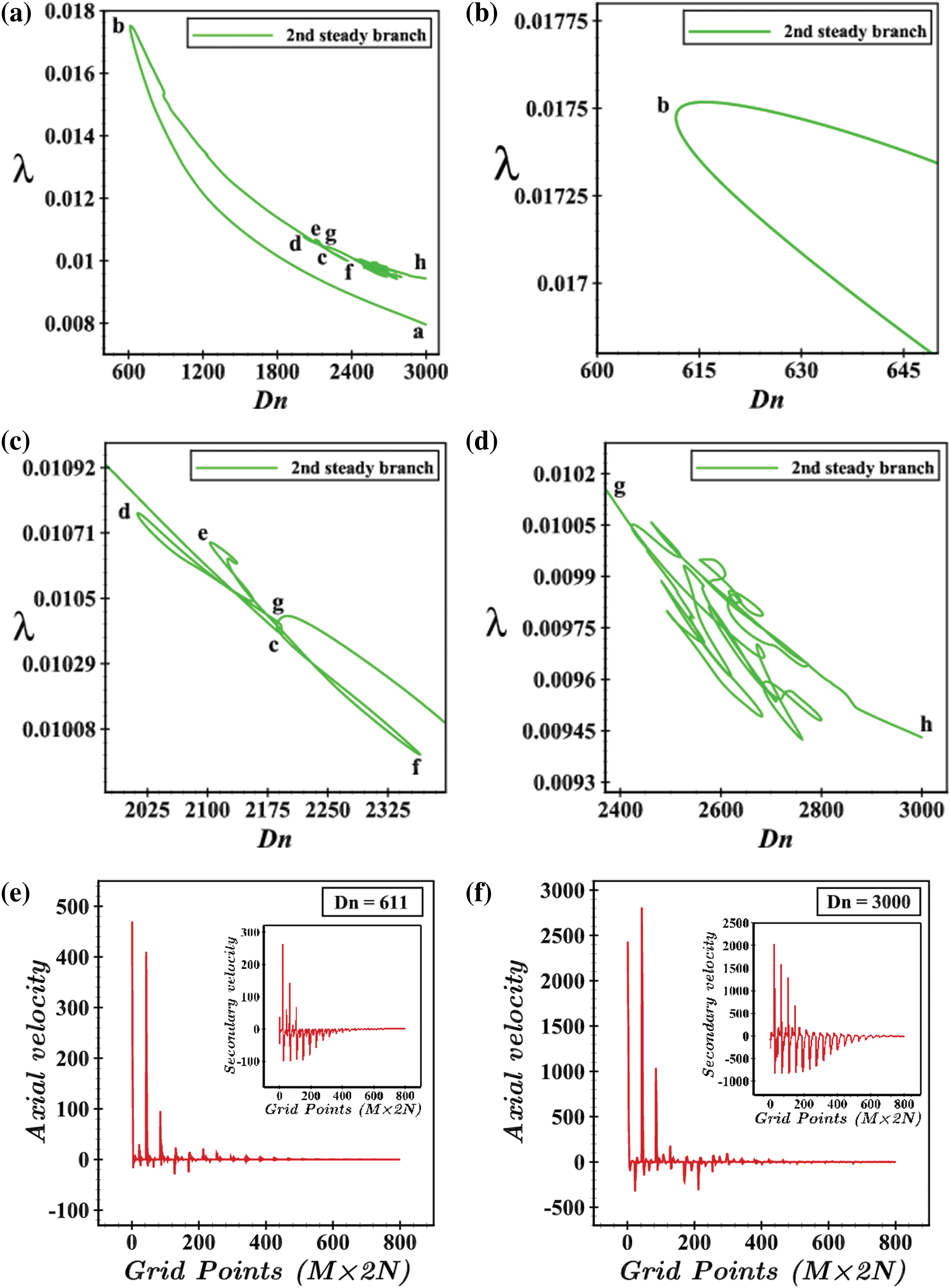
Figure 6: (a) 2nd steady solution branch; (b–d) are enlargements of (a) for 600 ≤ Dn ≤ 650, 2000 ≤ Dn ≤ 2350 and 2400 ≤ Dn ≤ 2850, respectively; (e) and (f) are axial velocity and secondary velocity distribution for Dn = 611 and 3000

The point b is very smooth as shown in enlarged Fig. 6b. The AVD and SFP for Dn = 611 and Dn = 3000 concerning grid points are shown in Fig. 6e,f, respectively. Exploring the velocity distribution, the changes are visible as compared to the 1st steady branch. Both the higher-pressure gradient and external heat are responsible for increasing the velocity. The 3rd SS branch occupying the range is portrayed in Fig. 7a. The branch starts at point a for Dn = 3000 (λ = 0.00802) and finally reaches the point k (Dn = 3000, λ = 0.00887) amidst many turnings that are shown with appropriate zoom Fig. 7b–d for the ranges , , and , respectively. AVD and SFP for and concerning grid points are shown in Fig. 7e,f, respectively, and can be observed the presence of a high-pressure gradient and the impact of external heat.

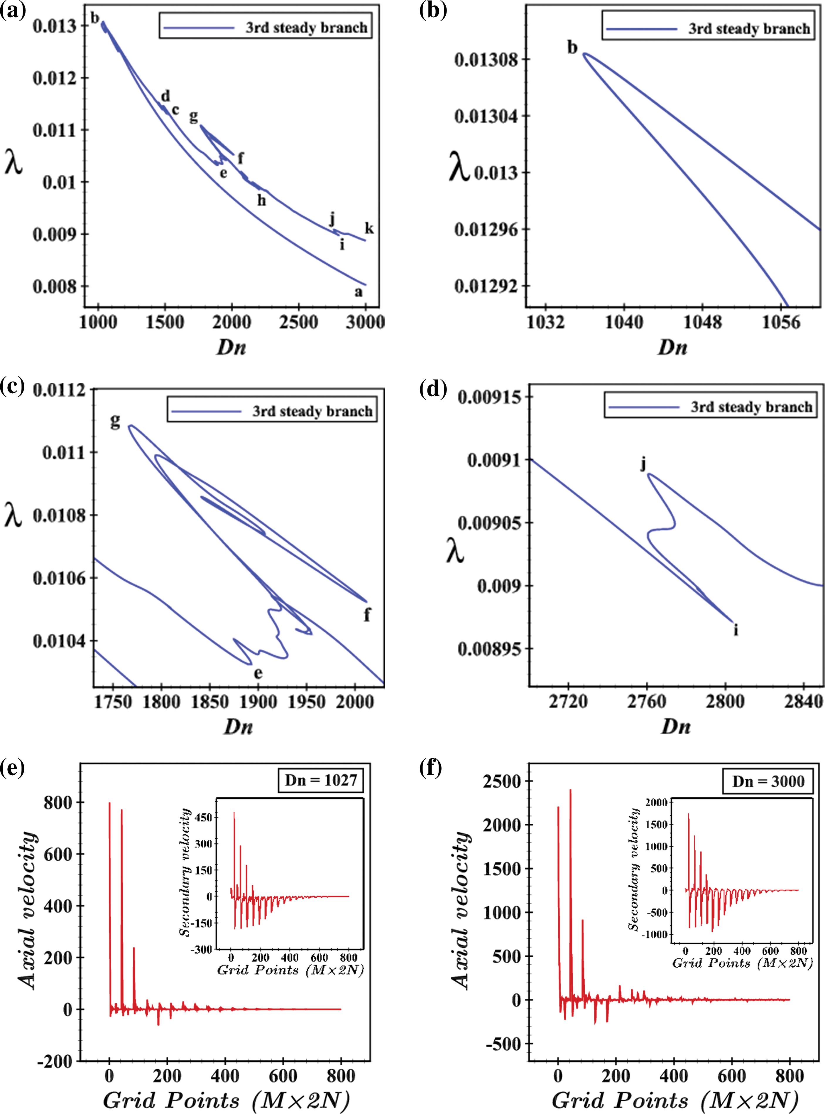
Figure 7: (a) 3rd steady solution branch; (b–d) are enlargements of (a) for various Dn region; (e) and (f) are axial velocity and secondary velocity distribution for Dn = 1027 and 3000

The fourth SS branch is located in the region of which commences from (point a) and finally reaches point j (Dn = 3000, λ = 0.00876), and is displayed in Fig. 8a. Then extends for increasing λ and decreasing Dn up to point b (Dn = 805.2, λ = 0.01496) with two strict turnings at Dn = 801.95 (λ = 0.01494) and Dn = 813.83 (λ = 0.01479). From here, the branch then prolongs in reverse direction and gets to point c (Dn = 1085.25, λ = 0.01354) followed by point d (Dn = 1006.12, λ = 0.01399). After reaching point e (Dn = 1578.01, λ = 0.01157), the branch becomes more intertwined between point f (Dn = 1499.84, λ = 0.01197) and g (Dn = 1603.55, λ = 0.01148) (see Fig. 8c). Fig. 8d shows the transition from point h by a strict turning tends to point i. The distribution of axial velocity and secondary velocity at Dn = 801 and concerning grid points is shown in Fig. 8e,f, respectively. Typical contours of SF are drawn in Fig. 9 for various Dean numbers where it can be explored that the branch starts with asymmetric 2-vortex solutions at Dn = 3000 and remained 2-vortex up to . The whole branch consists of asymmetric 2- to 12-vortex solutions at various Dn’s.

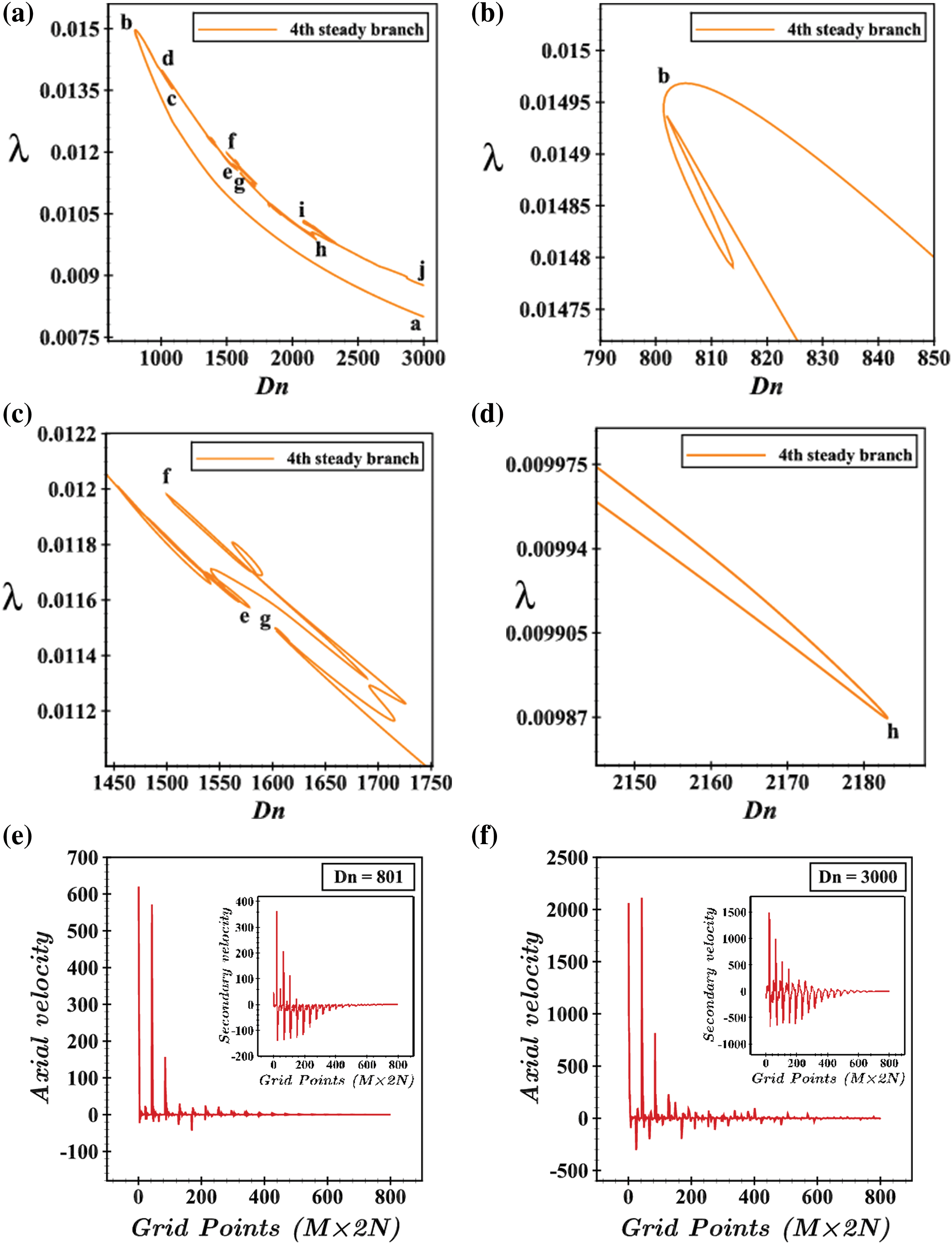
Figure 8: (a) 4th steady solution branch; (b–d) are enlargements of (a) for various Dn regions; (e) and (f) are axial velocity and secondary velocity distribution for Dn = 801 and 3000

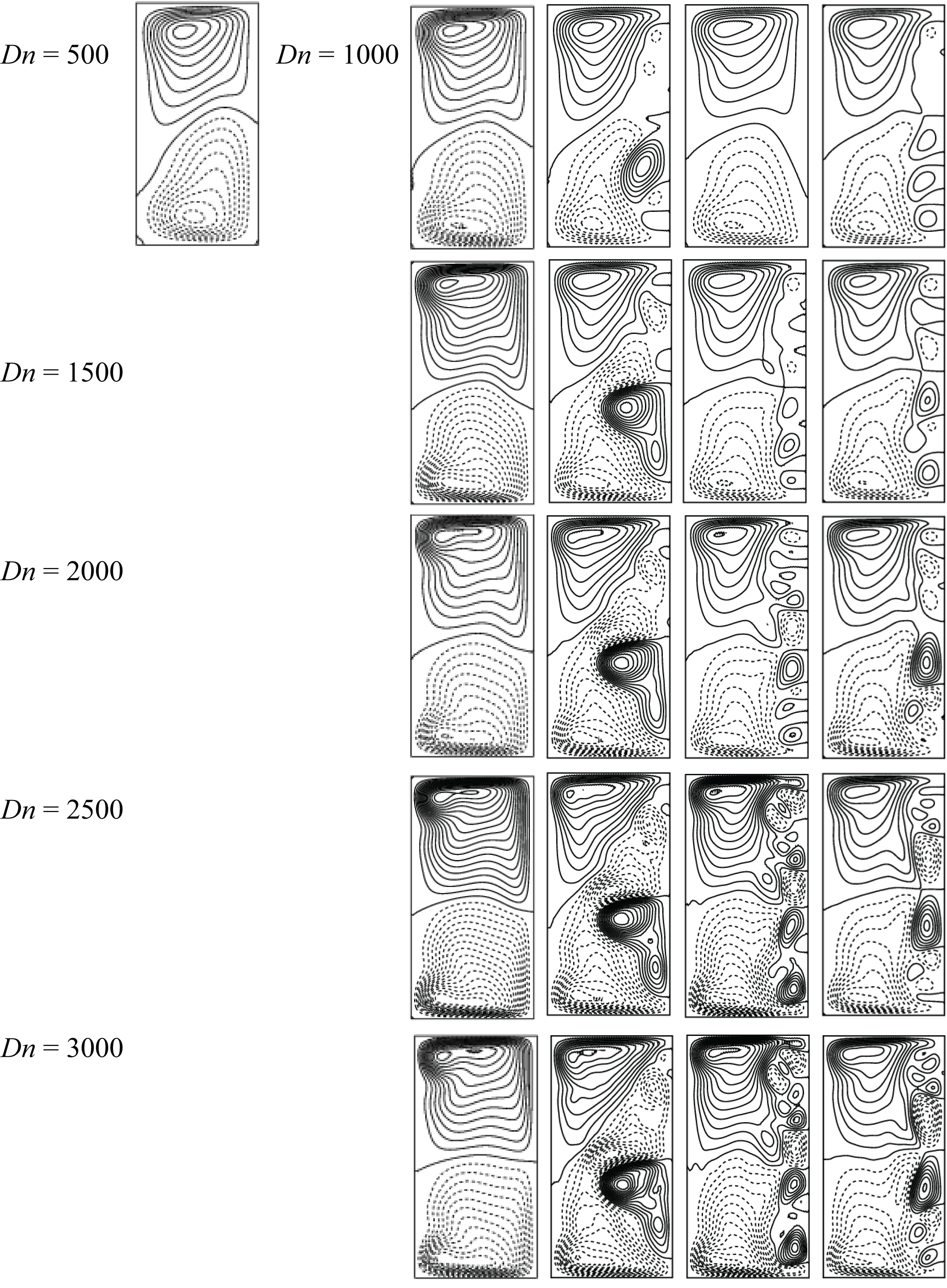
Figure 9: Vortex generation on various branches of steady solutions with respect to Dn

The stability of the steady solutions is influenced by the thermal effects, particularly the heating-induced buoyancy force. In the present study, the bottom and outer walls of the duct are heated, while the upper and inner walls are kept at room temperature. This temperature gradient creates a buoyancy force that interacts with the centrifugal force, further complicating the flow dynamics. The heating-induced buoyancy force can either stabilize or destabilize the flow, depending on the balance between the thermal and centrifugal effects.

4.2 Branch-Wise Vortex Comparison

Here, we have analyzed the vortex structure and the number of secondary vortices at a specific Dn’s throughout every SS branch as shown in Figs. 9 and 10, respectively, which means how the vortices looked like in each branch at a fixed Dn and how many vortices have arisen. The formation of secondary vortices is driven by the interaction between the centrifugal force and the pressure gradient. As the fluid flows through the curved duct, the centrifugal force pushes the fluid toward the outer wall, creating a pressure gradient across the duct. This pressure gradient induces secondary flows, which manifest as vortices. The number and arrangement of these vortices depend on the Dean number and the thermal effects. At higher Dean numbers, the flow becomes more unstable, leading to the formation of multiple vortices and complex flow patterns. At first, we investigated for Dn = 500, where we observed that the only first SS branch contains this value and obtained 2-vortex at Dn = 500. The next investigated value is Dn = 1000 where it can be seen that a 2-vortex structure exists in the 1st and 3rd branches while 7 vortices exist in the 2nd and 4th branches. Then, we found 2, 8, and 11 vortices for Dn = 1500 for the consecutive branches. The number of vortices in the 1st steady branch remained unchanged up to Dn = 2000 whereas decreased by 2-vortices in the 2nd branch but one more vortex was created in the 3rd and 4th branches. The same number of vortices are attained in the 1st and 3rd branches, is declined to 5-vortex in the 2nd, and is increased by one in the 4th branch for Dn = 2500. Except for the third branch (the highest 12-vortex are found), the other three branches have continued with the identical number of vortices for Dn = 3000.

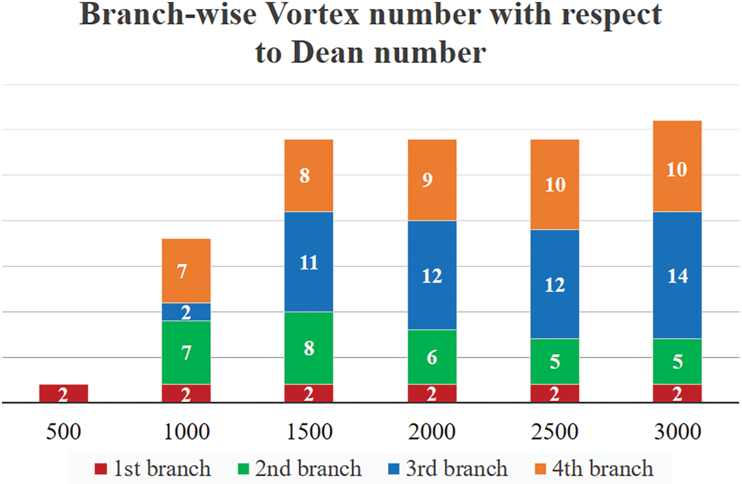
Figure 10: Branch-wise number of secondary vortices with respect to Dn

4.3 Time Advancement Flow Analysis

This section delves into the non-linear characteristics of unsteady flow (UF) through a loosely bent rectangular duct by examining the time evolution of the flow resistance coefficient (λ) across a range of Dn. The analysis reveals various flow regimes, including steady-state, periodic, multi-periodic, and chaotic flows, each characterized by distinct vortex structures and flow patterns.

At a low Dean number (Dn = 10), the flow remains in a steady state, as shown in Fig. 11a. The axial velocity distribution (AVD) and secondary velocity distribution (SVD) for Dn = 10 are depicted in Fig. 11b. The AVD is directed towards the center of the duct, while the SVD decreases significantly when crossing grid number 450. This behavior is attributed to the low-pressure gradient and centrifugal force. The flow pattern, illustrated in Fig. 11c, consists of an asymmetric single-vortex solution. The steady-state flow persists up to Dn = 86, with the flow resistance coefficient (λ) decreasing to 0.06065. As the Dean number increases slightly beyond 86, a notable shift occurs in the UF pattern. At Dn = 86.5, the steady-state flow transitions to a periodic flow, as shown in Fig. 12a. The periodic oscillation is traced between specific time intervals, confirmed by the power spectrum density (P-S) in Fig. 12b. The grid-point-wise distribution of axial and secondary velocities for Dn = 86.5 is presented in Fig. 12c, showing increased velocity distributions due to the pressure gradient. The flow pattern for a single period () of oscillation is depicted in Fig. 12d, consisting of asymmetric 2-vortex solutions, with the upper vortex dominating over the smaller vortex from the lower wall of the duct.

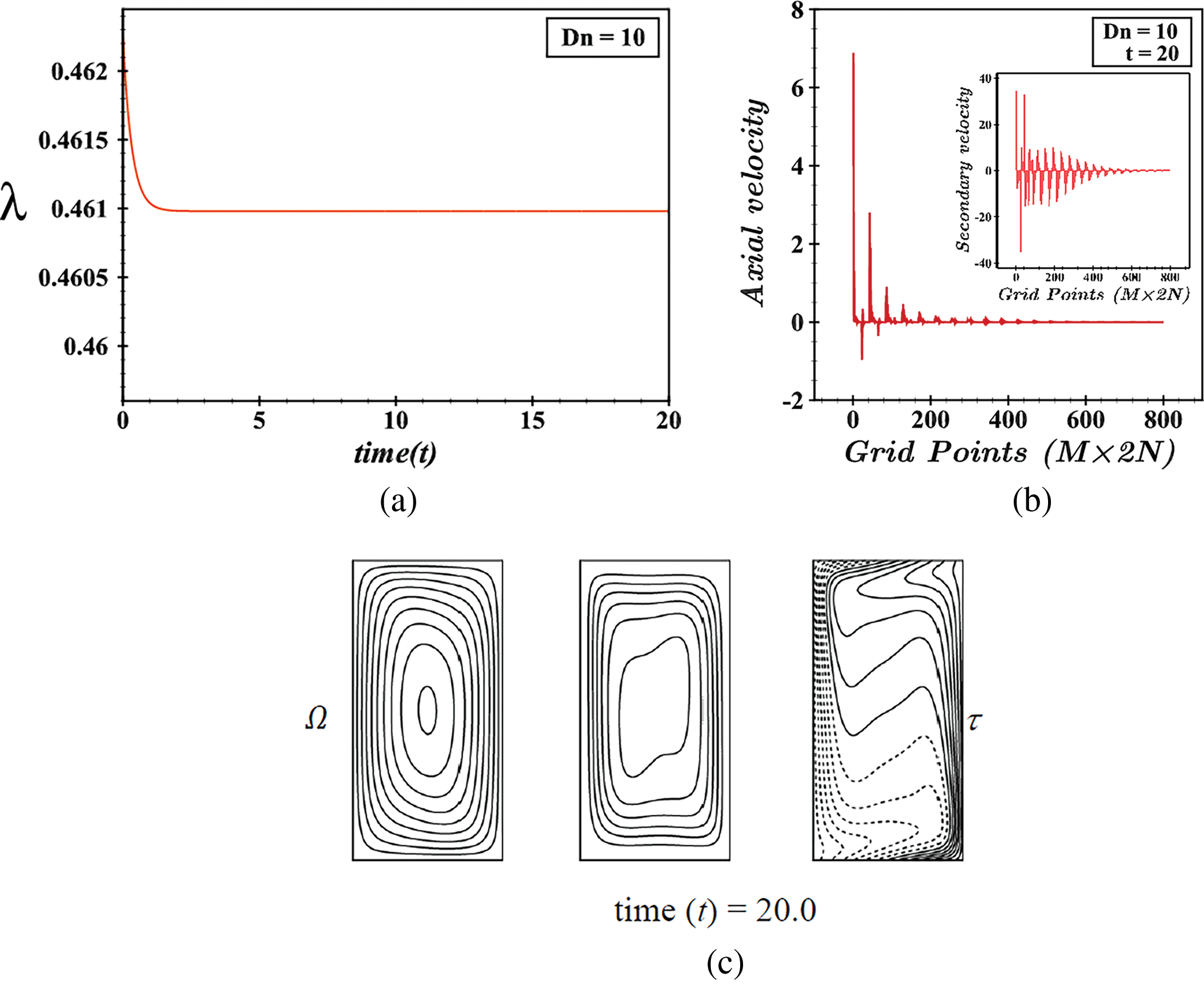
Figure 11: (a) Time progression, (b) grid-point wise axial and secondary velocity distribution, (c) contours of axial flow, secondary flow, and isotherms at t = 20.00 for Dn = 10

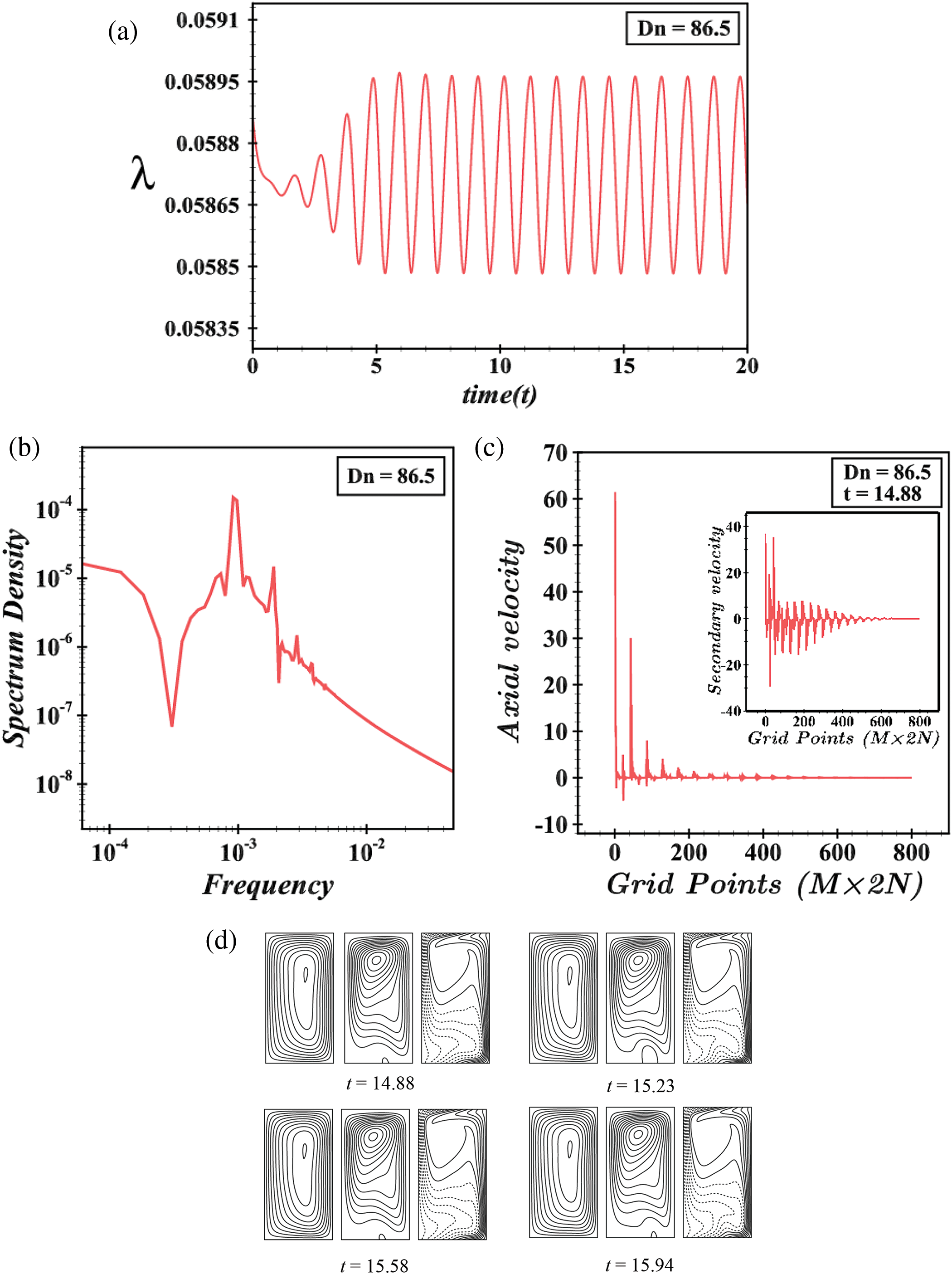
Figure 12: (a) Time progression, (b) power spectrum density, (c) grid-point-wise axial and secondary velocity distribution, (d) contours of axial flow, secondary flow, and isotherms for Dn = 86.5 at

The periodic flow becomes multi-periodic (M-P) for Dn = 202 as shown in Fig. 13a in the plane. The flow pulsates between and . To clear the obscurity of whether the flow is M-P or not, we draw the P-S of this TDF as shown in Fig. 13b. The elementary frequencies, their harmonics, and more lines spectrum confirm to us, that the flow is M-P. For Dn = 202 and at t = 17.32, the grid-point-wise AV and SV are sketched in Fig. 13c. The contours of axial flow (AF), SF, and isotherms for this M-P flow are presented in Fig. 13d for a single period of oscillation . It is seen that the SF is composed of asymmetric 2- and 3-vortex solutions. Due to the increase in temperature and pressure gradient in the lower and outer walls, two new vortices are generated; one from the lower wall and the other from the outer wall of the duct.

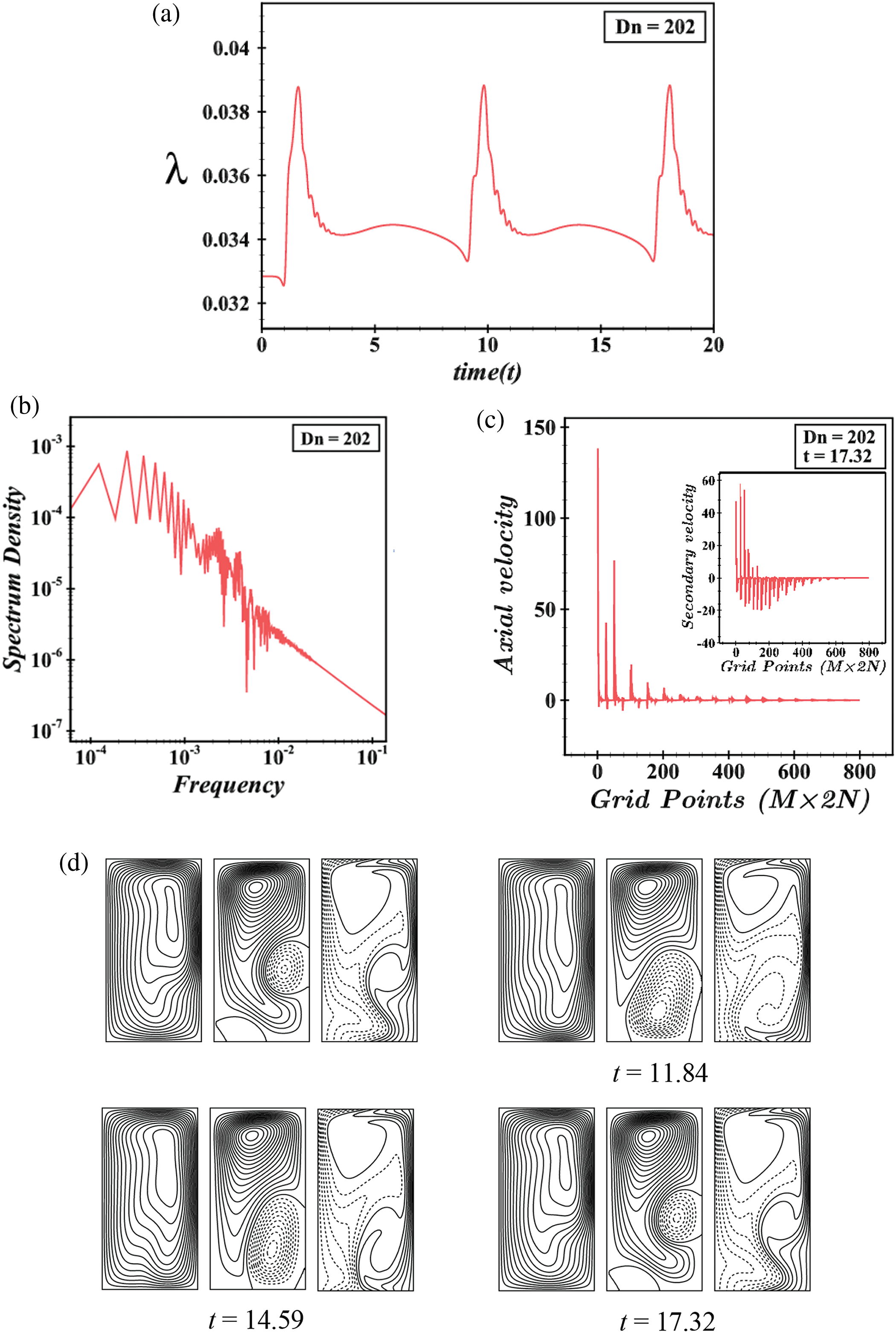
Figure 13: (a) Time progression, (b) power spectrum density, (c) grid-point-wise axial and secondary velocity distribution, (d) contours of axial flow, secondary flow, and isotherms for Dn = 202 at

We have studied the UF precisely to explore all possible solutions. It is interesting to see that the M-P flow again turns periodic for Dn = 400 with the period between and as depicted in Fig. 14a. Fig. 14b describes the P-S where it is seen that the flow is periodic. The AVD as explained grid-point-wise (reporting the SV in the same figure always) is depicted in Fig. 14c at t = 14.67. The flow patterns are presented in Fig. 14d, where it is exposed that the periodic flow is composed of an asymmetric 2-vortex solution. After a slight increase in the pressure gradient at Dn = 430, the flow transitions back to M-P, oscillating between specific time intervals with asymmetric 2- and 3-vortex solutions, as shown in Fig. 15a,d. The P-S in Fig. 15b confirms the M-P nature of the flow. The grid-point-wise AVD and SVD for Dn = 430 are illustrated in Fig. 15c, showing increased fluid velocity and temperature due to the influence of the outer wall of the duct. To visualize the fluctuating behavior of the unsteady solutions again, it is drawn for Dn = 500 as in Fig. 16a, where it is seen that the flow is chaotic with pulsates between and . To eliminate our doubt about whether it is periodic or chaotic, we exhibit P-S of TDF (see Fig. 16b). The flow can be defined as transitional chaos (Mondal et al. [27]). Also, the grid-point-wise velocity distribution of the axial flow and secondary velocity is depicted in Fig. 16c at t = 15.26. For a specific time interval, , the pattern fluctuation of AF, SF, and isotherms is shown in Fig. 16d, from which it can be seen that the SF is composed of asymmetric 4-vortex solutions. As much as increasing the pressure gradient for example Dn = 3000, the flow is remained unchanged and becomes more chaotic with 5- to 10-vortex solutions, which is termed strong chaos (Mondal et al. [27]) which means we have found no significant change except the strongest chaotic flow as depicted in Fig. 17a,d. The P-S of TDF and the grid-point-wise velocity distribution are displayed in Fig. 17b,c. Therefore, all the unsteady solutions are summarized by illustrating them as a percentage as well as vortex number. In the current investigation range of Dean number, the region of the steady-state flow is the periodic/multi-periodic flow interval is , and the rest of the region is for the chaotic flow with some transitions. The schematic representation of the percentage with vortex number is demonstrated in Fig. 18. From the figure, we observed that the maximum area holds the chaotic flow of approximately 86% with 2- to 10-vortex solutions while the steady-state flow holds a minimum area of approximately 3% with single and 2-vortex solutions and periodic flow consists of 2- and 3-vortex solution with 11% of the total flow region.

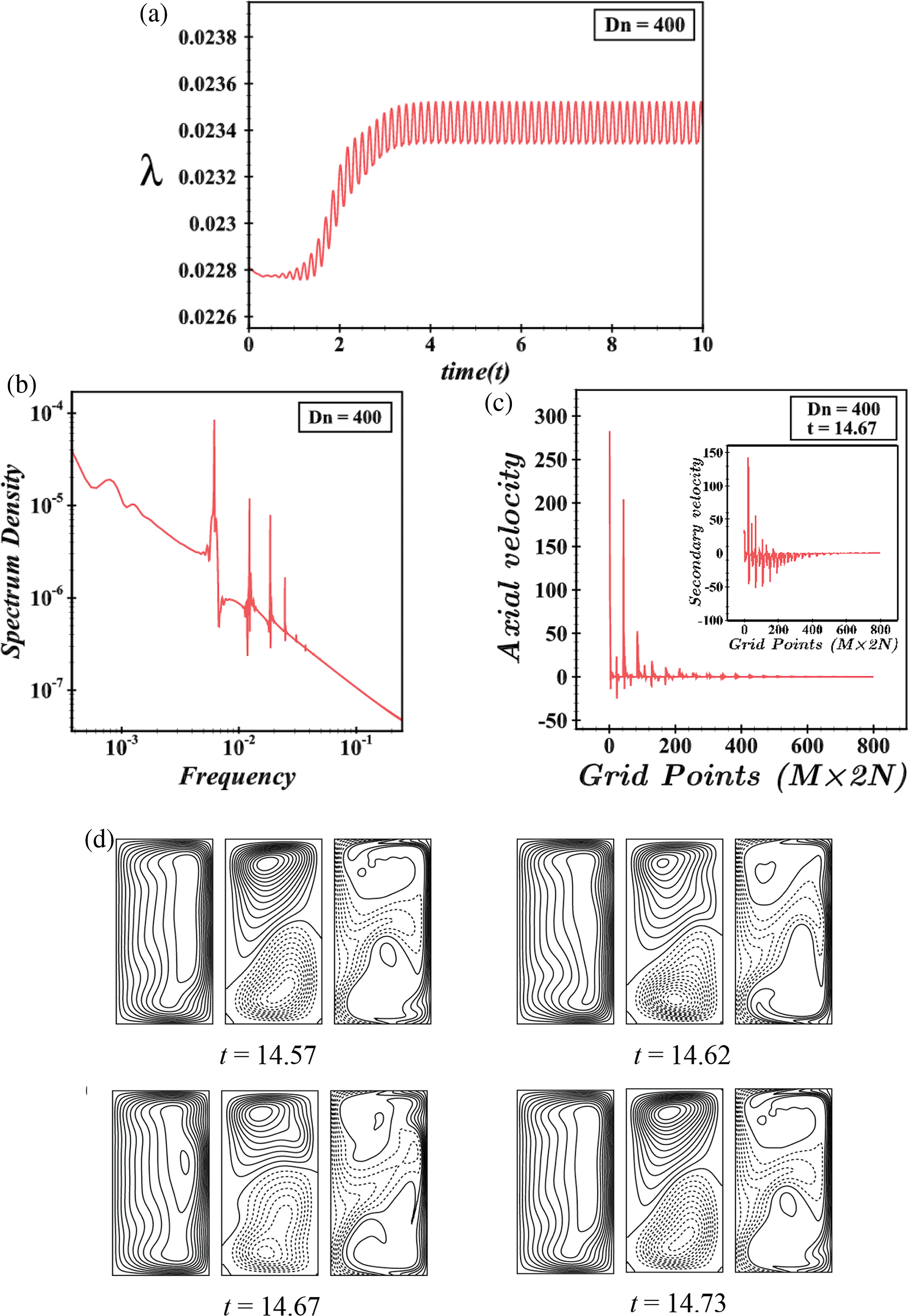
Figure 14: (a) Time progression, (b) power spectrum density, (c) grid-point wise axial and secondary velocity distribution, (d) contours of axial flow, secondary flow, and isotherms for Dn = 400 at

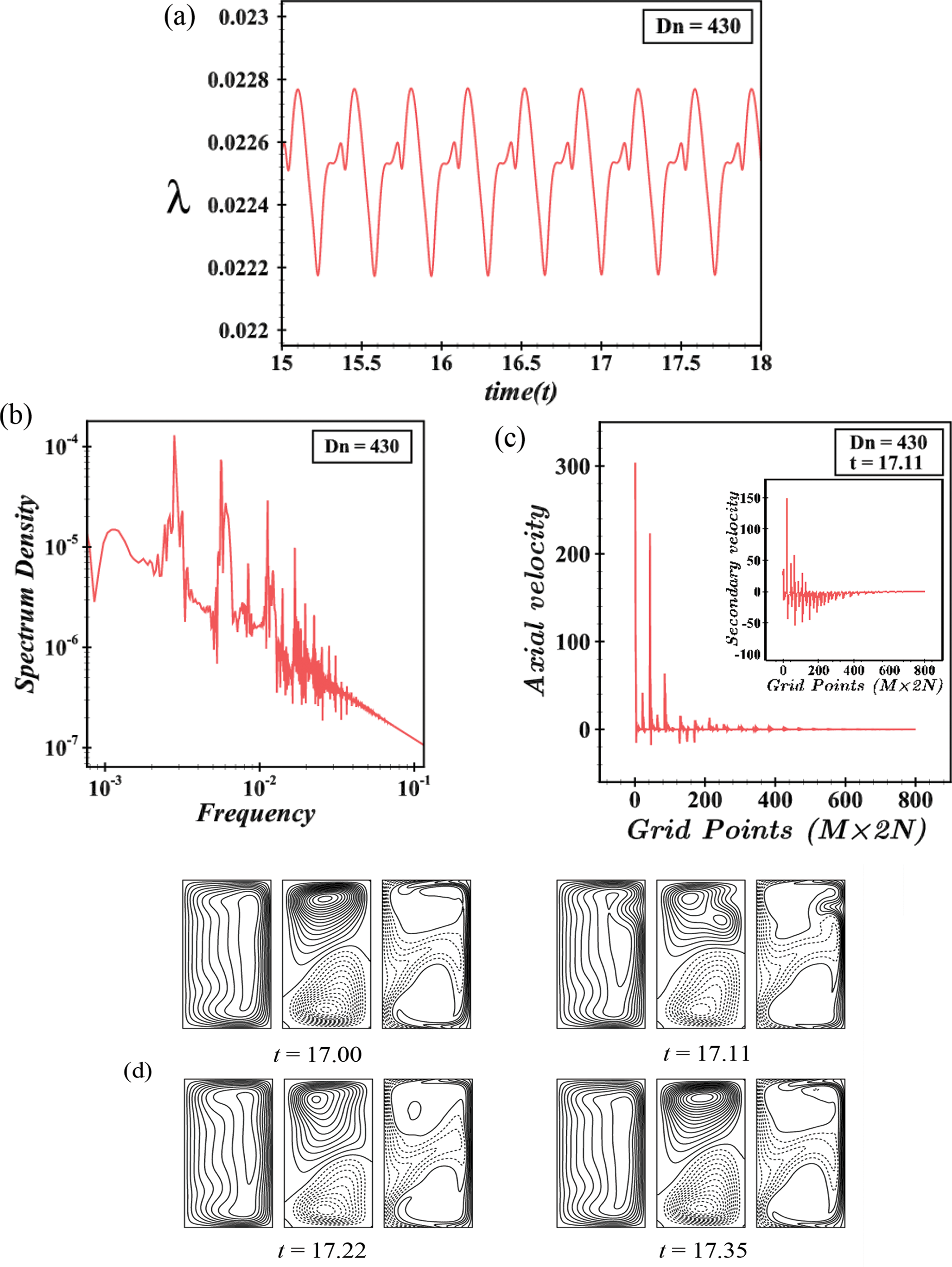
Figure 15: (a) Time progression, (b) power spectrum density, (c) grid-point-wise axial and secondary velocity distribution, (d) contours of axial flow, secondary flow, and isotherms for Dn = 430 at

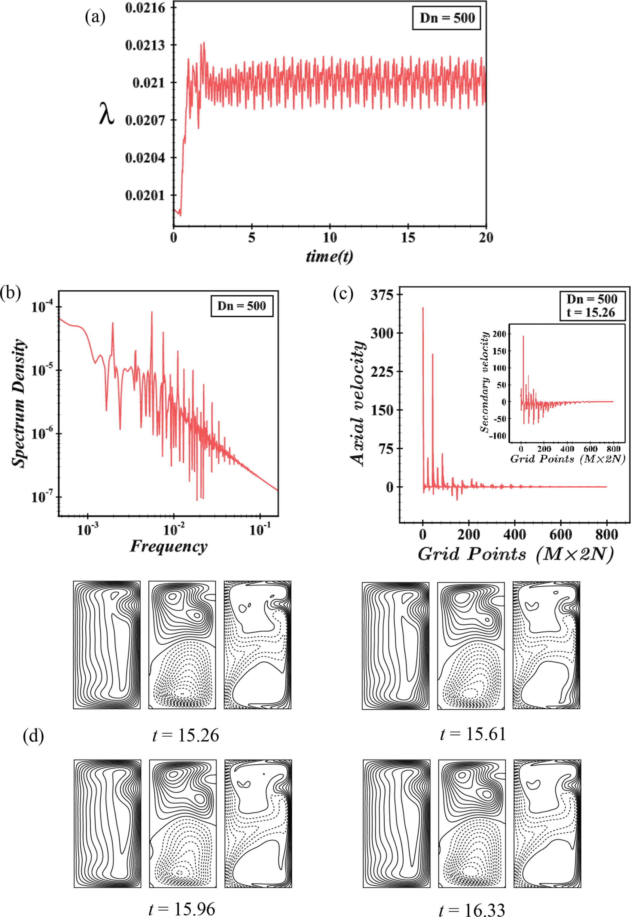
Figure 16: (a) Time progression, (b) power spectrum density, (c) grid-point-wise axial and secondary velocity distribution, (d) contours of axial flow, secondary flow, and isotherms for Dn = 500 at

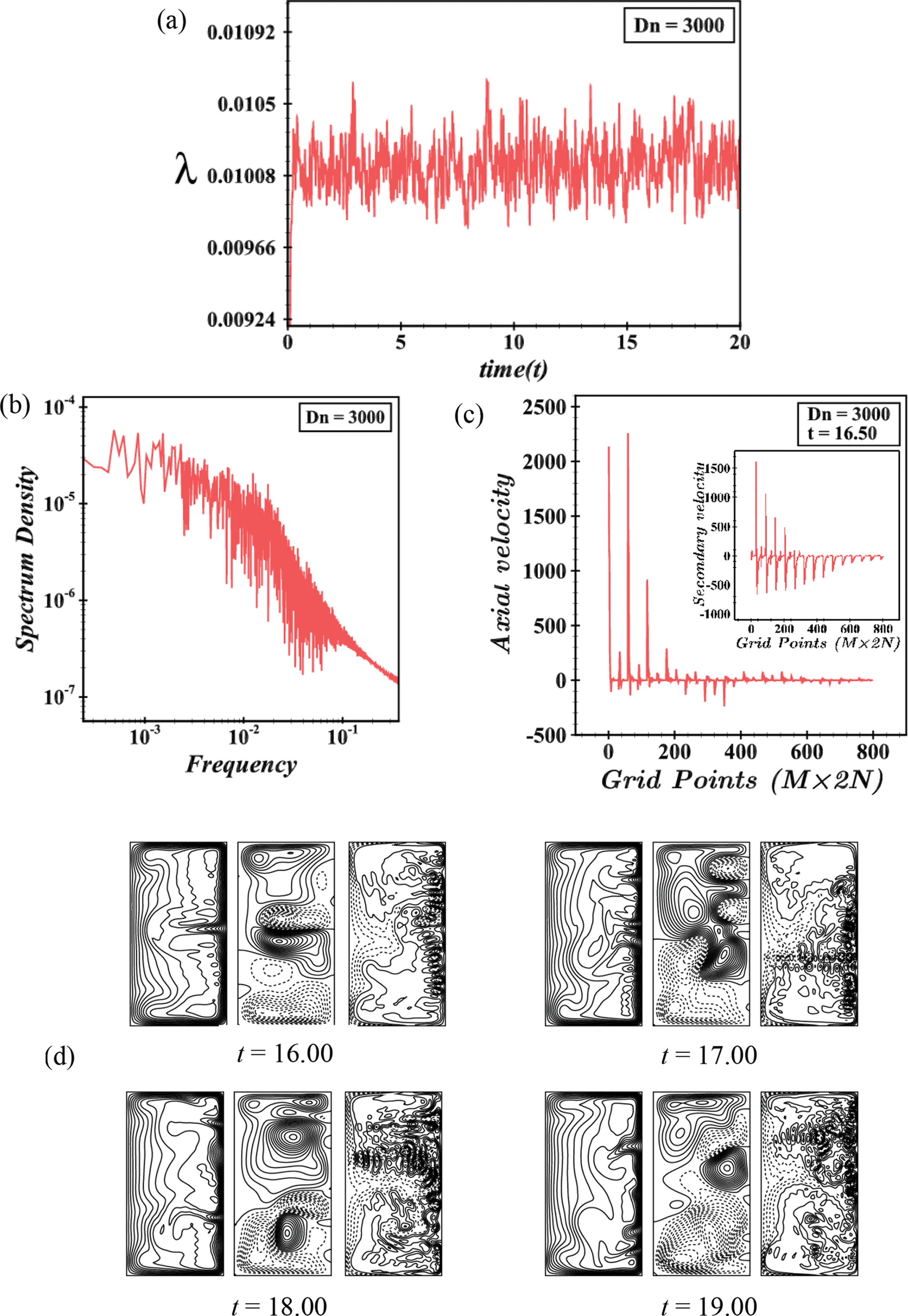
Figure 17: (a) Time progression, (b) power spectrum density, (c) grid-point-wise axial and secondary velocity distribution, (d) contours of axial flow, secondary flow, and isotherms for Dn = 3000 at

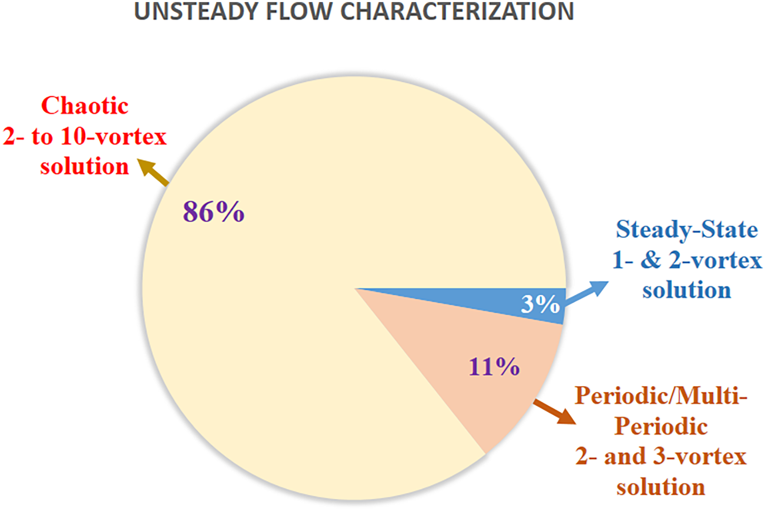
Figure 18: Unsteady flow percentage with number of secondary vortices

This time advancement flow analysis reveals the complex dynamics of unsteady flow in a curved rectangular duct, driven by the interplay between centrifugal force, pressure gradient, and thermal effects. The Dean number is crucial in determining the flow regime and stability of flow patterns. At low Dn’s, the flow remains stable with a single vortex structure due to the low-pressure gradient and centrifugal force. As the Dn increases, the flow transitions to a periodic regime characterized by oscillations and asymmetric 2-vortex solutions influenced by pressure gradient and thermal effects. Further increase in the Dean number leads to multi-periodic flow with more complex oscillations and multiple vortex structures, resulting from the interaction between centrifugal force and thermal effects. At higher Dn’s, the flow becomes chaotic with irregular oscillations and complex vortex structures driven by strong centrifugal force and thermal effects, leading to multiple vortices and flow instabilities. By remembering these transitions and dynamics, one can substantially optimize the fluid flow and heat transfer in engineering applications involving curved ducts.

4.4 Heat Transfer

4.4.1 Variation of Nusselt Number with the Dean Number

Convective heat transfer (CHT) is explored in two unique ways for the separated warmed sidewalls. Since we have pondered both steady and unsteady streams in this paper, so Nusselt number (Nu) as a sign of CHT is executed for both types of solutions. A distinct methodology is driven to compute Nu from the UF and the way is for a specific Dn, above all else, time evolution (TE) is examined and afterward, Nu is averaged from the whole time-advancement flow. In Fig. 19, the expansion of Nu is introduced in the (Dn-Nu) plane, in which the blue and red solid lines depict the Nu for SS and the representative type of squares and stars outline the time average of Nu for unsteady solutions for both cooled and heated walls separately. The analysis shows that Nu for steady-state and time-averaged unsteady solutions coincide when the flow is steady. Initially, the value of Nu is similar at the start of the pressure gradient. However, as Dn increases, Nu for the cooled walls decreases until the flow reaches a steady state, while it increases for the heated walls. When the flow transitions to another solution, such as periodic or chaotic, a steady rise in Nu is observed in the cooled walls, and a substantial growth in Nu is noticed in the heated walls. This behavior is attributed to the increased turbulence and mixing of the fluid, which generates more vortices in the secondary flow, enhancing heat convection.

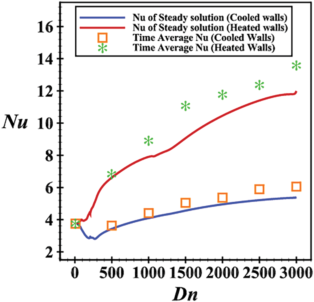
Figure 19: Variation of Nu with Dn for cooling and heated walls

Here, the variation of Nu with the Dean number (Dn) reveals important insights into the heat transfer characteristics of the flow. At low Dn, the flow is primarily laminar, and the heat transfer is dominated by conduction. As Dn increases, the flow becomes more turbulent, enhancing convective heat transfer. This transition is marked by an increase in Nu, particularly for the heated walls, where the temperature gradient drives the convective currents. The decrease in Nu for the cooled walls at higher Dn can be attributed to the stabilization of the flow, where the secondary vortices reduce the temperature gradient near the walls, leading to lower heat transfer rates. Conversely, the heated walls experience an increase in Nu due to the intensified mixing and turbulence, which enhance the heat transfer efficiency.

4.4.2 Temperature Gradients

The analysis of heat transfer through temperature gradients (TG) helps to understand the direction and magnitude of heat transfer within the duct. TG on the cooled and heated edges are calculated for an extended range of Dn , as illustrated in Fig. 20a,b. On the cooled walls, the value of decreases in the middle of the duct with the increase of Dn, due to the secondary flow advection in the external direction caused by centrifugal force. Simultaneously, TG tends to rise monotonically over the entire duct except for the central portion. On the heated walls, shows an upward trend in the central region, influenced by the outward secondary flow moving inward. Summarizing for cooled walls, the TG decreases in the middle of the duct with increasing Dn, indicating that the secondary flow advection moves the cooler fluid towards the outer regions. This behavior is driven by the centrifugal force, which pushes the fluid outward, reducing the temperature gradient in the central region, and for heated walls, the TG shows an upward trend in the central region suggesting that the heated fluid is being pushed inward by the secondary flow. This inward movement enhances the temperature gradient near the walls leading to higher heat transfer rates.

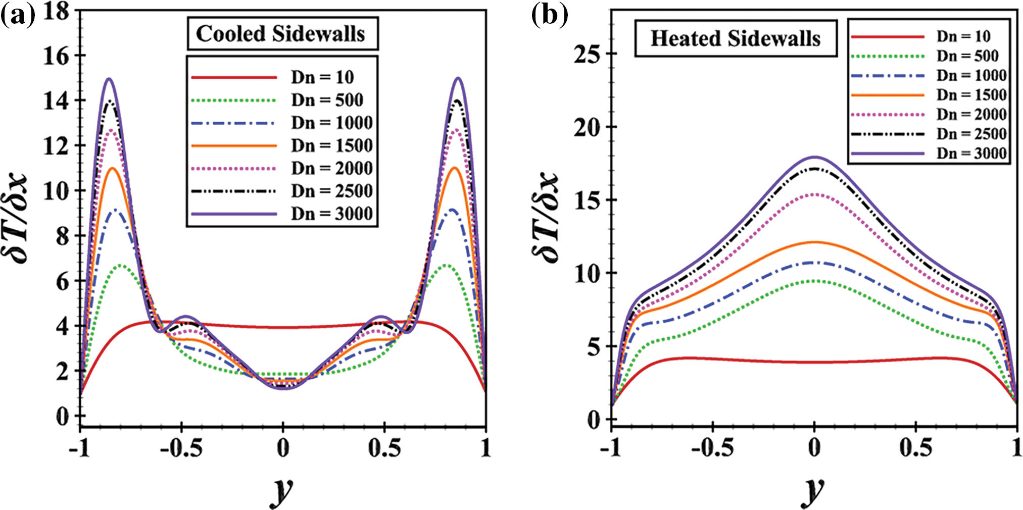
Figure 20: Temperature gradients (a) at the cooled walls; (b) at the heated walls

5  Discussions

This study builds on existing research in the field of fluid dynamics by exploring complex flow behaviors and heat transfer in a loosely bent rectangular duct. The literature has established the importance of bifurcation in curved channels, where centrifugal forces generate secondary flows and drive the transition from steady to chaotic regimes (Dean [8,9] and Yanase et al. [18]). Previous studies have also highlighted several types of bifurcation, including Hopf, pitchfork, and saddle-node, and analyzed the impact of pressure gradients and wall heating on flow stability (Benjamin [10,11], Mondal et al. [22]). However, a key limitation in the existing literature is the lack of grid-point-specific velocity distribution analysis, which limits the understanding of local flow behaviors.

The present study addresses this gap by providing detailed velocity profiles along steady solution branches for various Dn’s. This granular approach offers a novel perspective on flow stability and vortex structures across multiple bifurcation branches. In addition to steady-state bifurcations, the study captures the transition to time-dependent unsteady flows (UF), where chaotic and multi-periodic flows enhance heat convection through turbulent mixing. These findings build on previous research (Hasan et al. [17]) by demonstrating how chaotic flow regimes driven by centrifugal and buoyancy forces significantly boost heat transfer efficiency. Another contribution of this study is the numerical modelling of energy distribution along different flow regimes. By examining the Nusselt number (Nu) and temperature gradients, the results highlight how flow transitions—from steady-state to periodic and chaotic regimes—influence heat convection. This detailed numerical analysis provides practical insights for engineering applications, such as optimizing the Dean numbers to maximize heat transfer in heat exchangers and cooling systems. The use of a spectral-based numerical approach further strengthens the robustness of the findings, validating them against experimental data from previous studies (Chandratilleke [29], Sugiyama et al. [31]).

6  Conclusion

In this study, we introduce a detailed spectral-based numerical method to analyze the bifurcation structure of steady solutions and the behavior of unsteady flows in a curved rectangular duct. This approach allows for a precise examination of flow features and energy distribution, providing new insights into the complex dynamics of fluid flow in curved geometries. Unlike previous studies, our work emphasizes the interplay between centrifugal force, pressure gradient, and thermal effects, highlighting their combined impact on flow stability and heat transfer. The key findings and contributions of our work are summarized as follows:

•   We identified four branches of asymmetric steady solutions, each characterized by distinct vortex structures. The bifurcation analysis revealed the transition points between different flow regimes providing a deeper understanding of the stability and behavior of fluid flow in curved ducts. Exploring the number of secondary vortices in the steady branches, the findings are only a 2-vortex solution in the 1st steady branch; 2- and 5- to 8-vortex solution in the 2nd steady branch; 2- to 12-vortex solution in the 3rd steady branch; and 2- and 6- to 10-vortex solution in the 4th steady branch. The formation of secondary vortices is driven by the interaction between centrifugal force and thermal effects, leading to complex flow patterns.

•   Investigating the non-linear behavior of unsteady flow phenomena, the result can be organized as steady-state →periodic→multi-periodic→periodic→chaotic. The transitions between these regimes are influenced by the pressure gradient and thermal effects, resulting in a wide range of flow patterns and vortex structures. Steady-state flow lies on with single- and 2-vortex solution, periodic and multi-periodic flow involved in the region with asymmetric 2- and 3-vortex solution and the rest of the region of this investigation is a chaotic flow region which is accounted for 2- to 10-vortex solution.

•   Convective heat transfer (CHT) study finds the relation between the Nusselt number (Nu) with the Dean number and reveals significant differences in heat transfer efficiency between steady and unsteady flows. We found that chaotic flows enhance heat transfer due to increased turbulence and mixing, while steady-state flows exhibit lower heat transfer rates. The analysis of temperature gradients further elucidated the direction and magnitude of heat convection, highlighting the role of secondary vortices in redistributing thermal energy.

Future Perspectives

Since this study is based on hydrodynamic flow, we are planning to extend it to Magneto-hydrodynamics (MHD) fluid flow. For the same configuration, instead of using temperature differences between vertical walls, we may apply the electric potential difference to create radial currents and impose an axial magnetic field parallel to vertical walls. The interaction between radial currents and axial magnetic field generates Lorentz force that can drive the flow in the azimuthal direction. Morescro et al. [33] studied experimentally this kind of MHD flow and stability properties were explicitly outlined. Another aim to extend this study is to introduce nanofluids [34,35] and heat transfer properties for flow in a curved channel.

Acknowledgement: None.

Funding Statement: Rabindra Nath Mondal (R. N. Mondal), one of the authors, would like to gratefully acknowledge the financial support from Jagannath University, Dhaka to conduct this research work (Ref. No. JnU/Research/Pro/2021-2022/Science/21), URL: www.jnu.ac.bd (accessed on 26 November 2024).

Author Contributions: The authors confirm contribution to the paper as follows: study conception and design: Rabindra Nath Mondal and Sreedham Chandra Adhikari; data collection: Sreedham Chandra Adhikari; analysis and interpretation of results: Rabindra Nath Mondal and Sreedham Chandra Adhikari; draft manuscript preparation: Rabindra Nath Mondal, Giulio Lorenzini, Sidhartha Bhowmick and Sreedham Chandra Adhikari; supervision: Rabindra Nath Mondal and Giulio Lorenzini. All authors reviewed the results and approved the final version of the manuscript.

Availability of Data and Materials: The data that support the findings of this study are available from the corresponding author upon request.

Ethics Approval: Not applicable.

Conflicts of Interest: The authors declare no conflicts of interest to report regarding the present study.

References

1. Anisur R, Xu W, Li K, Dou HS, Khoo BC, Mao J. Influence of magnetic force on the flow stability in a rectangular duct. Adv Appl Math Mech. 2019;11(1):24–37. doi:10.4208/aamm.OA-2018-0142. [Google Scholar] [CrossRef]

2. Sykes JP, Gallagher TP, Rankin BA. Effects of Rayleigh-Taylor instabilities on turbulent premixed flames in a curved rectangular duct. Proc Combust Inst. 2021;38(4):6059–66. doi:10.1016/j.proci.2020.06.146. [Google Scholar] [CrossRef]

3. Zhang K, Wang Y, Tang H, Yang L. Magnetohydrodynamic flow regimes in an annular channel. Phy Fluids. 2022;34(2):027114. doi:10.1063/5.0080885. [Google Scholar] [CrossRef]

4. Khan SA, Baig MA, Muneer R, Suheel JI, Faheem M. Benefit of Mach number and expansion level on the flow development in a cylindrical tube diameter of 18 mm. Mater Today Proc. 2021;47:6220–6. [Google Scholar]

5. Sheard GJ, Fitzgerald MJ, Ryan K. Cylinders with square cross-section: wake instabilities with incidence angle variation. J Fluid Mech. 2009;630:43–69. doi:10.1017/S0022112009006879. [Google Scholar] [CrossRef]

6. Miles A, Bessaïh R. Heat transfer and entropy generation analysis of three-dimensional nanofluids flow in a cylindrical annulus filled with porous media. Int Com Heat Mass Trans. 2021;124(9):105240. doi:10.1016/j.icheatmasstransfer.2021.105240. [Google Scholar] [CrossRef]

7. Sheard GJ, Ryan K. Pressure-driven flow past spheres moving in a circular tube. J Fluid Mech. 2007;592:233–62. doi:10.1017/S0022112007008543. [Google Scholar] [CrossRef]

8. Dean WR. Note on the motion of fluid in a curved pipe. Phill Mag. 1927;4(20):208–23. [Google Scholar]

9. Dean WR. Fluid motion in a curved channel. Proc R Soc Lond A. 1928;121(787):402–20. [Google Scholar]

10. Benjamin TB. Bifurcation phenomena in steady flows of a viscous fluid. I. Theory. Proc R Soc Lond A. 1978;359(1696):1–26. [Google Scholar]

11. Benjamin TB. Bifurcation phenomena in steady flows of a viscous fluid. II. Experiments. Proc R Soc Lond A. 1978;359(1696):27–43. [Google Scholar]

12. Bara BM, Nandakumar K, Masliyah JH. An experimental and numerical study of the Dean problem: flow development towards two dimensional multiple solutions. J Fluid Mech. 1992;244(1):339–76. doi:10.1017/S0022112092003100. [Google Scholar] [CrossRef]

13. Wang L, Yang T. Bifurcation and stability of forced convection in curved ducts of square cross-section. Int J Heat Mass Trans. 2004;47(14–16):2971–87. doi:10.1016/j.ijheatmasstransfer.2004.03.002. [Google Scholar] [CrossRef]

14. Ghosh S, Mukhopadhyay S. Flow and heat transfer of nanofluid over an exponentially shrinking porous sheet with heat and mass fluxes. Propuls Power Res. 2018;7(3):268–75. doi:10.1016/j.jppr.2018.07.004. [Google Scholar] [CrossRef]

15. Chen KT, Yarn KF, Chen HY, Tsai CC, Luo WJ, Chen CN. Aspect ratio effect on laminar flow bifurcations in a curved rectangular tube driven by pressure gradients. J Mech. 2017;33(6):831–40. doi:10.1017/jmech.2017.93. [Google Scholar] [CrossRef]

16. Adhikari SC, Chanda RK, Bhowmick S, Mondal RN, Saha SC. Pressure-induced instability characteristics of a transient flow and energy distribution through a loosely bent square duct. Energy Eng. 2021;119(1):429–51. [Google Scholar]

17. Hasan MS, Mondal RN, Islam MZ, Lorenzini G. Physics of coriolis-energy force in bifurcation and flow transition through a tightly twisted square tube. Chin J Phy. 2023;77(9):1305–30. doi:10.1016/j.cjph.2021.11.023. [Google Scholar] [CrossRef]

18. Yanase S, Nishiyama K. On the bifurcation of laminar flows through a curved rectangular tube. J Phy S Jap. 1988;57(11):3790–95. doi:10.1143/JPSJ.57.3790. [Google Scholar] [CrossRef]

19. Mondal RN, Uddin MS, Yanase S. Numerical prediction of non-isothermal flow through a curved square duct. Int J Fluid Mech Res. 2010;37(1):85–99. doi:10.1615/InterJFluidMechRes.v37.i1.60. [Google Scholar] [CrossRef]

20. Li Y, Wang X, Yuan S, Tan SK. Flow development in curved rectangular ducts with continuously varying curvature. Exp Therm Fluid Sci. 2016;75:1–15. doi:10.1016/j.expthermflusci.2016.01.012. [Google Scholar] [CrossRef]

21. Dolon SN, Hasan MS, Lorenzini G, Mondal RN. A computational modeling on transient heat and fluid flow through a curved duct of large aspect ratio with centrifugal instability. Euro Physic J Plus. 2021;136(4):1–27. doi:10.1140/epjp/s13360-021-01331-0. [Google Scholar] [CrossRef]

22. Mondal RN, Adhikari SC, Chanda RK, Ghalambaz M, Islam MS. Effects of pressure gradient on fluid flow and energy distribution in a bending square channel. J Nanofluids. 2023;12(8):1–14. doi:10.1166/jon.2023.2090. [Google Scholar] [CrossRef]

23. Guo G, Kamigaki M, Inoue Y, Nishida K, Hongou H, Koutoku M, et al. Experimental study and conjugate heat transfer simulation of pulsating flow in straight and 90° curved square pipes. Energies. 2021;14(13):3953. doi:10.3390/en14133953. [Google Scholar] [CrossRef]

24. Adhikari SC, Hasan MS, Rouf RA, Lorenzini G, Mondal RN. A Computational modeling on two-dimensional laminar flow and thermal characteristics through a strongly bent square channel. AIP Adv. 2023;13(11):115007. doi:10.1063/5.0158615. [Google Scholar] [CrossRef]

25. Hussen S, Islam MR, Mondal RN. Numerical study of solution structure and nonlinear behavior of Dean flow with vortex structure in a bending square duct. Phy Fluids. 2023;35(11):117116. doi:10.1063/5.0175180. [Google Scholar] [CrossRef]

26. Gottlieb D, Orszag SA. Numerical analysis of spectral methods: theory and applications. S Ind Appl Math. 1977;26:172. [Google Scholar]

27. Mondal RN, Kaga Y, Hyakutake T, Yanase S. Bifurcation diagram for two-dimensional steady flow and unsteady solutions in a curved square duct. Fluid Dyn Res. 2007;39(5):413–46. [Google Scholar]

28. Wang L, Pang O, Cheng L. Bifurcation and stability of forced convection in tightly coil ducts: multiplicity. Chaos Soliton Fract. 2005;26:337–52. [Google Scholar]

29. Chandratilleke TT. Secondary flow characteristics and convective heat transfer in a curved rectangular duct with external heating. In: 5th World Conference on Experimental Heat Transfer, Fluid Mechanics and Thermodynamics, 2001; Thessaloniki, Greece. [Google Scholar]

30. Chandratilleke TT. Numerical prediction of secondary flow and convective heat transfer in externally heated curved rectangular ducts. Int J Therm Sci. 2003;42(2):187–98. [Google Scholar]

31. Sugiyama S, Hayashi T, Yamazaki K. Flow characteristics in the curved rectangular channels: visualization of secondary flow. Bull JSME. 1983;26(216):964–69. [Google Scholar]

32. Chandratilleke TT, Nadim N, Narayanaswamy R. Analysis of secondary flow instability and forced convection in fluid flow through rectangular and elliptical curved ducts. Heat Transf Eng. 2013;14:1237–48. doi:10.1080/01457632.2013.777249. [Google Scholar] [CrossRef]

33. Moresco P, Alboussiere T. Experimental study of the instability of the Hartmann layer. J Fluid Mech. 2004;504:167–81. doi:10.1017/S0022112004007992. [Google Scholar] [CrossRef]

34. Varzaneh AA, Toghraie D, Karimipour A. Comprehensive simulation of nanofluid flow and heat transfer in straight ribbed microtube using single-phase and two-phase models for choosing the best conditions. J Therm Analy Calorim. 2020;139(1):701–20. doi:10.1007/s10973-019-08381-8. [Google Scholar] [CrossRef]

35. Liu X, Toghraie D, Hekmatifar M, Akbari OA, Karimipour A, Afrand M. Numerical investigation of nanofluid laminar forced convection heat transfer between two horizontal concentric cylinders in the presence of porous medium. J Therm Anal Calorim. 2020;141(5):2095–108. doi:10.1007/s10973-020-09406-3. [Google Scholar] [CrossRef]