Evaluating Effect of Magnetic Field on Nusselt Number and Friction Factor of Fe₃O₄-TiO₂/Water Nanofluids in Heat-Sink Using Artificial Intelligence Techniques

1  Introduction

A heat-sink is a passive device that dissipates heat produced by an electrical or mechanical device away from the device and into a fluid medium, usually air or liquid coolant. The device allows for temperature control and, for instance, computers employ heat sinks to cool their central processor units. Mini- and micro-component development has increased, especially in electronic devices, due to the constraints of conventional liquid or air-cooling techniques and the small physical dimensions of the electronic devices. The development of mini-scale technology, including mini- and micro-components, is one way to improve heat transfer. Researchers have looked closely at heat transfer and fluid pressure drops through mini and microchannels.

The heat sink performance can be augmented by using high thermal conductivity fluids (nanofluids), which were formally introduced in the scientific literature by Choi [1]. By using these nanofluids, the heat transfer coefficient may be augmented. Earlier relevant research work revels that, by using different mono nanofluid, the is augmented [2,3]. Even the researchers a have also observed an enhanced with the use of hybrid nanofluids [4–6]. Kumar et al. [7] used water-mixed Al2O3-TiO2 hybrid nanofluid in a mini-channel heat sink and found numerically and experimentally enhancement of 8.5% and 12.8%, respectively, with for Al2O3 (10:0) hybrid nanofluid. The enhancement of 15.6% was observed by Kumar et al. [8] by using Al2O3-multi-walled carbon nanotube (MWCNT)/water nanofluids in a mini-channel heat-sink. The heat transfer, and pressure drop increase of 63.13% and 20.35% was observed by Ahammed et al. [9] by using graphene–alumina hybrid nanofluids in a mini-channel. Nimmagadda et al. [10] observed an enhanced when using aluminum oxide (Al2O3), silver (Ag), and hybrid (Al2O3 + Ag) hybrid nanofluids in a micro-channel. Nimmagadda et al. [11] noted augmented heat transfer using single-walled carbon nanotubes (SWCNT), Au Al2O3, Ag, and Al2O3-Ag hybrid nanofluids in a micro-channel at low Reynolds numbers. Nanda Kishore et al. [12] obtained Nusselt number enhancement for Al2O3-CuO hybrid nanofluids in wavy mini-channels. Murali Krishna et al. [13] determined a 13.2% and 23.07% increase in Nusselt number for Cu-Al2O3/water hybrid nanofluid compared to Cu/water and Al2O3/water mono nanofluids, respectively, at 2.5% vol. in a microchannel heat-sink. Ongoing research indicates that hybrid nanofluids can be superior to mono-nanofluids in terms of thermal performance.

The artificial neural network (ANN) is one of the soft computing tools that can be used for modeling or predicting hybrid nanofluids data efficiently. Previous studies related to the use of ANN for mono and hybrid nanofluids heat transfer are surveyed here. The natural convection heat transfer data of Cu/water mono nanofluids in a cavity was predicted using ANN by Santra et al. [14]. Nucleate pool boiling heat transfer data related to TiO2/water nanofluids was predicted through multilayer perceptron (MLP), generalized regression neural network (GRNN), and radial basis networks (RBF) by Balcilar et al. [15]. The overall heat transfer coefficient and pressure drop data applicable to Mn-Zn/water hybrid nanofluids in a double pipe heat exchanger were predicted using ANN by Bahiraei et al. [16]. Water-diluted TiO2/water nanofluids in a mini-channel were predicted by Naphon et al. [17] with the Levenberg-Marquardt Backward-propagation (LMB) training ANN algorithm and found a 1.25% deviation between measured and predicted data. Tafarroj et al. [18] noted a 0.3% and 0.2% average relative error with ANN for heat transfer coefficient and Nusselt number, respectively, of TiO2/water nanofluid in a microchannel heat sink. Khosravi et al. [19], using ANN, obtained heat transfer enhancement of 134% by using graphene-platinum/water hybrid nanofluid in a microchannel heat sink. Esfe [20] used ANN to analyze the experimental data of Ag/water nanofluid in a heat exchanger for the predictions and noted 99.76% and 99.54% accuracy for the Nusselt number and pressure drop, respectively. Yasir et al. [21] investigated the heat conduction of homogeneous-heterogeneous reactions in the axisymmetric flow of Oldroyd-B materials and obtained improved fluid velocity near the cylinder surface. Yasir et al. [22] investigated the thermal transport characteristics of water-based Al2O3/Ag hybrid nanofluids over a vertical stretching/shrinking surface by a MATLAB (MATrix LABoratory) based numerical model and they determined an increased friction drag and decrease of thermal heat transfer with an increase of nanoparticle concentrations.

The heat transfer of mono and hybrid magnetic nanofluids can be tuned by with the effect of an external magnetic field. The influence of the external magnetic field was studied by Ghofrani et al. [23] for Fe3O4, and they noted the values of can increase up to 27.6% for Fe3O4/water nanofluids by increasing the external magnetic field. For a magnetic field of 1200 Gauss Ashjaee et al. [24] found an increase for of 38%, but with no magnetic field, the increase was only 14% for Fe3O4/water nanofluid flow in a heat-sink, as compared to the base fluid. Riaz Khan et al. [25] analyzed the skin friction coefficient, frictional drag, and heat transfer of Cu-Al2O3/H2O-C2H6O2 hybrid nanofluid over a stretched surface based on the boundary conditions of aligned magnetic field and nonlinear radiation and they found that hybrid nanofluids provide better rate of with less frictional drag. Tekir et al. [26] obtained a 14% increase of for Fe3O4-Cu/water hybrid nanofluid under a fixed magnetic field. Alsarraf et al. [27] found an increment of 109.31% and 25.02% for Nusselt number and pressure drop, respectively, for a fixed magnetic field of 0.9% magnetite with 1.35% CNT hybrid nanofluid with a Re of 500. Mehrali et al. [28] observed increase of 82% and entropy generation reduction of 41% for graphene/Fe3O4 ferro-nanofluid under a magnetic field. Sundar et al. [29] used water-dispersed Fe3O4-TiO2 in a mini-heat-sink and noticed at 2 vol%, the Nusselt number increase of 38.16% without magnetic field and 88.93% under a magnetic field of 1000 Gauss.

A review of previous studies on the application of post-processing techniques to predict the heat transfer coefficient, Nusselt number, and friction factor reveals that, in spite of a large number of artificial neural networks (ANNs), there is no particular study devoted to the determination of the optimal ANN structure, including the optimal number of hidden layers, the optimal number of neurons in each layer, the optimal weighting of the neurons, and the optimal transmission function. To present the best structure among the evaluated structures, researchers have examined a limited number of neural network structures. The current study investigated three ANN structures with varying numbers of neurons in each hidden layer, combining various transfer functions in the first and second hidden layers, and independently optimizing the transfer function, in addition to performing laboratory tests to determine the heat transfer coefficient, Nusselt number, and friction factor of water dispersed Fe3O4-TiO2/water hybrid nanofluids in a mini-heat-sink with the effect of magnetic fields. ANOVA t-test analysis is used to determine the best ANN technique. Through the NN analysis, a regression equation was also developed.

2  Artificial Neural Network

There has been a growing trend of nanofluid studies in the last few decades, and a large portion of the research work has been dealing with nanofluid flow and heat transfer for enhanced performance of thermal devices. In summary, most nanofluid studies related to the ANN were related to the properties. Therefore, the ANNs were developed from previous experimental data on each nanofluid properties. Now we are trying to extend the ANN for heat transfer data of nanofluids in a thermal device. The procedure included the gathering of experimental data and performing the data fitting through different ANN algorithms, and developing new polynomial correlations.

2.1 Back Propagation Neural Network

The backpropagation neural network (BPNN) comprises an input layer hidden layers and an output layer. BPNN is a specific type of feedforward ANN that utilizes the backpropagation algorithm for training. Backpropagation enables error feedback and more effective weight updates, leading to improved learning and performance in the network. Making a well-executed BPNN model is all about finding the right training procedure and tweaking parameters like the transfer function, hidden layer count, and hidden neuron count. The layout of back propagation neural network architecture is presented in Fig. 1.

Figure 1: Layout of back propagation neural network architecture

In this work, we examined three different backpropagation algorithms to train the ANN, and they are Levenberg-Marquardt (LM), Broyden–Fletcher–Goldfarb–Shanno Quasi Newton (BFGS), and Variable Learning Rate Gradient Descent (VLGD) methods.

(i)   Levenberg-Marquardt trained ANN: Levenberg-Marquardt (LM) is an algorithm commonly used for training neural networks, particularly in the context of solving nonlinear least squares problems. The LM algorithm combines the features of Gauss-Newton and gradient descent methods to achieve efficient and robust optimization. It aims to minimize the error between the model’s predicted output and the actual output by adjusting the network’s weights.

Given a neural network with weights represented by the vector w, and a set of training data , , where, is the input and is the corresponding desired output, the goal is to find the optimal weights that minimize the error between the network’s predicted output and the actual output.

Let be the output of the neural network for input and weights . The error between the predicted output and the desired output can be defined as:

(1)

The overall error of the network can be computed as the sum of the squared errors over all training examples:

(2)

The LM algorithm aims to find the optimal weights that minimize this error. It does so by iteratively updating the weights based on the gradients of the error function.

At each iteration, the LM algorithm calculates the Jacobian matrix J, which represents the partial derivatives of the network’s output with respect to the weights. The Jacobian matrix is defined as:

(3)

where, is the index of the training example and is the index of the weight.

The LM algorithm then solves the following linear system of equations:

(4)

where, is the weight update, is the damping factor (a regularization parameter), is the transpose of the Jacobian matrix, and is the vector of errors.

The weight update is computed using various methods, such as direct inversion of the system of equations or iterative methods like the conjugate gradient method.

Finally, the weights are updated as:

(5)

The LM algorithm iteratively performs these steps until a stopping criterion is met, such as a maximum number of iterations or reaching a desired level of error. By iteratively updating the weights based on the gradients of the error function, the LM algorithm aims to find the optimal weights that minimize the error and improve the network’s fit to the training data.

(ii)   BFGS Quasi-Newton trained ANN: The Broyden-Fletcher-Goldfarb-Shanno (BFGS) algorithm is a popular optimization method used in conjunction with backpropagation for training neural networks. It belongs to the class of Quasi-Newton methods, which aim to approximate the Hessian matrix (second derivative matrix) of the error function without explicitly computing it. The key idea behind the BFGS algorithm is to construct an approximation of the inverse Hessian matrix using information from the gradients of the error function at different iterations. This approximation is updated iteratively to improve its accuracy.

At each iteration, the algorithm computes the gradient vector g, which represents the first derivatives of the error function with respect to the weights. It then updates the weights by solving the following equation:

(6)

where, is the estimate of the inverse Hessian matrix at iteration , and is the weight update.

The BFGS algorithm updates the inverse Hessian matrix estimate using the following formula:

(7)

where, is a scalar that controls the curvature of the Hessian approximation, , and are the differences between consecutive weight updates and gradient vectors, respectively.

The weight update, is then computed as:

(8)

The BFGS algorithm iteratively performs these steps until a stopping criterion is met, such as reaching a desired level of error or a maximum number of iterations.

(iii)   Variable Learning Rate Gradient Descent algorithms (VLGD) trained ANN: The variable learning rate gradient descent algorithm adjusts the learning rate for each parameter in a backpropagation neural network (BPNN) based on the historical gradients. It aims to give more weight to parameters that have smaller updates and less weight to parameters with larger updates. The key idea behind this is to scale the learning rate inversely proportional to the sum of the squared gradients accumulated over all previous iterations. By doing so, it effectively dampens the learning rate for frequently updated parameters and amplifies the learning rate for parameters that have infrequent updates. It updates weight in three steps as follows:

(1)   Initialization:

•   Initialize the weights and biases (θ) of the BPNN with small random values, and Initial learning rate .

•   Initialize the sum of squared gradients for each parameter to zero.

(2)   Training Iterations:

•   For each training example in the dataset.

•   Perform forward propagation to compute the network’s output y.

•   Calculate the error between the predicted output and the true output.

•   Perform backpropagation to compute the gradients of the weights and biases .

•   For each parameter (weight or bias) in the network.

•   Accumulate the squared gradient by adding the square of the gradient with the sum of squared gradients for that parameter .

•   Compute the learning rate for the current parameter using the accumulated squared gradient: learning rate = .

•   where the epsilon term is a small constant added to avoid division by zero.

•   Update the parameter using the learning rate and the corresponding gradient: .

(3)   Repeat the training iterations until convergence or a maximum number of iterations is reached.

The flow chart of the ANN algorithm is given in Fig. 2. The input, output, and layers of the proposed neural network architecture are mentioned in Fig. 3.

Figure 2: Flow chart of the proposed ANN

Figure 3: Architecture of the proposed ANN

3  Data for ANN Training

A vast number of processing units known as neurons make up the ANN. ANNs are primarily made up of neurons, which are linked to networks by a series of connections, each of which has a distinct weight. The weight values of an ANN have a significant impact on its performance. The data of Sundar et al. [29] related to the Fe3O4-TiO2/water hybrid nanofluids data were considered in this study. The experimental setup and heat sink (test section) details of the work by Sundar et al. [29] are reported in Fig. 4a and b, respectively.

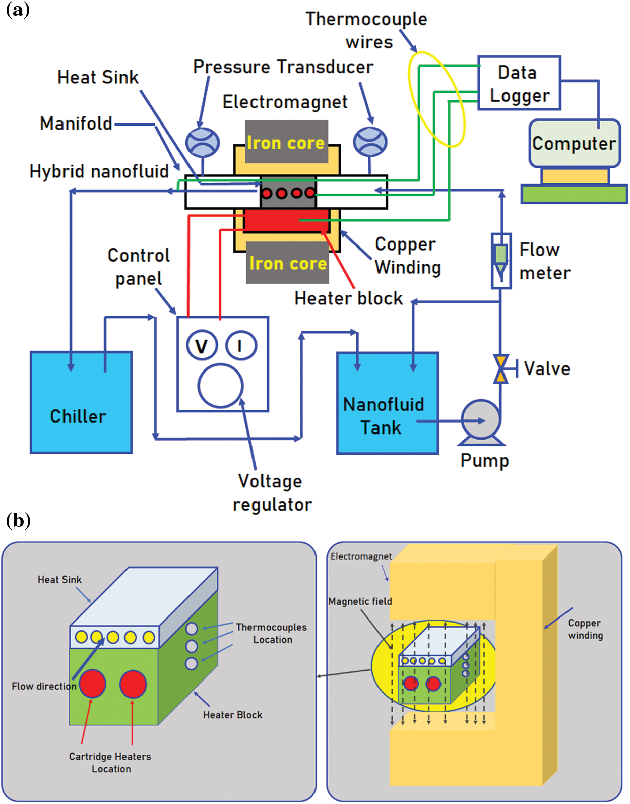
Figure 4: (a) Experimental setup, and (b) test section details (Sundar et al. [29])

In the ANN algorithms, Reynolds number, Prandtl number, volume concentrations, and magnetic field were considered input parameters, whereas, heat transfer coefficient, Nusselt number, and friction factor were taken as output parameters. The data of Sundar et al. [29] used for the ANN studies. As already stated, the three ANN models (LM, BFGS, and VLGD) were used for training, testing, and validation of the data. Over the entire data, 70% of data is used for training, 15% for testing, and the remaining 15% of the data is used for validation.

4  Results and Discussion

In this study, the three neural network algorithms—LM, BFGS, and VLGD were used to analyze the output parameters. Through the algorithms, we determined the mean square error (MSE), root-mean-square error (RMSE), and correlation coefficient (R2), which are defined as follows [19]:

(9)

(10)

(11)

where, is the number of experimental data, is the experimental data assigned to Nusselt number, heat transfer, and friction factor, respectively, and is the Nusselt number, heat transfer, and friction factor, respectively, analyzed by the algorithm. Moreover, is the mean value of the output parameters, is the number of observations, and is the mean value of error.

4.1 Heat Transfer Coefficient

Compared to traditional gradient-based methods, like gradient descent, the BFGS algorithm can converges faster, and it can handle the problems more effectively. By approximating the inverse Hessian matrix, it incorporates second-order information about the error surface, which improves the optimization process. The choice between LM, BFGS, and VLGD methods depends on the specific requirements of the neural network training task, such as the nature of the problem, memory constraints, and computational resources available. The back-propagation network has four inputs and one output layer for each analysis, those are connected by using hidden layers. The 10 hidden layers were considered for all the output data. The weight and bias of each neuron in hidden layers are optimized using three algorithms and their results are compared. To train the network, 70% of the data is used for training and 30% is for validation and testing of the algorithms.

Fig. 5 shows the predicted heat transfer results using the LM method for Fe3O4-TiO2 hybrid nanofluids. The training state plot, best validation performance, and error histogram are reported in Fig. 5a–c. From the figures, it can be observed that the gradient of the solution is 360.6037 at epoch 94. This indicates that the solution converged very smoothly without disturbing the data. Under the same epoch of 94, the validation checks are 6, and the Mu value is 1 (Fig. 5a). The best validation performance is 577.0856 as seen in Fig. 5b at epoch 88; also, it clearly shows the merging of training, validation, testing, and the best performance meeting at epoch 88. The error histogram with 20 Bins is shown in Fig. 5c, and it indicates an error of −2.756.

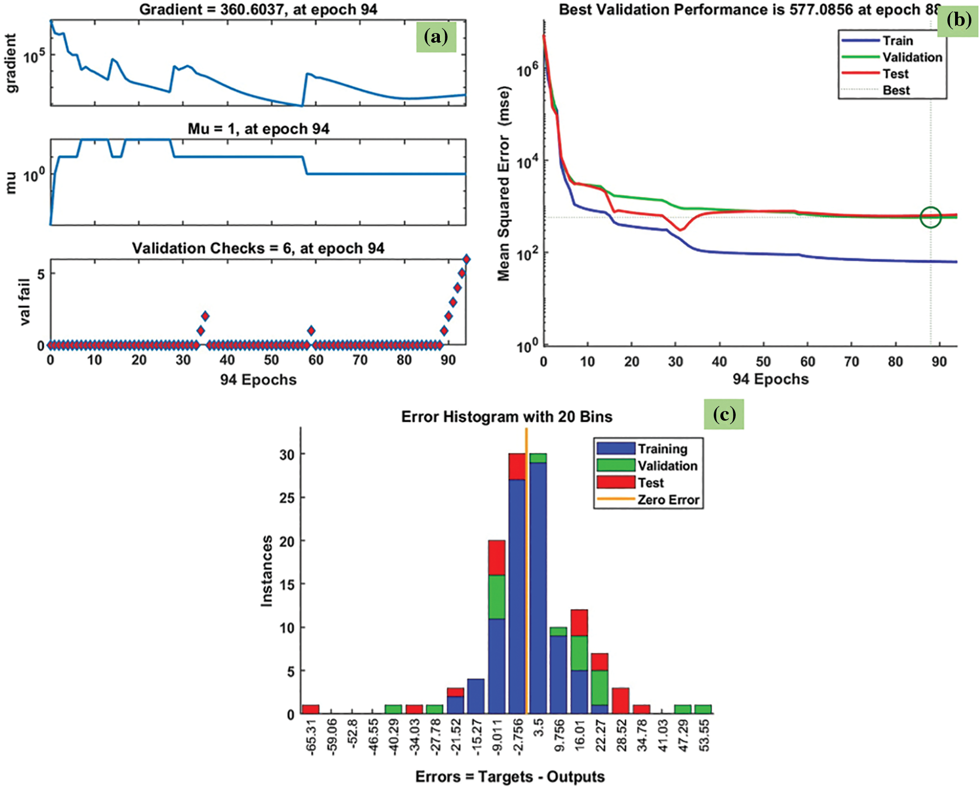
Figure 5: LM results of heat transfer coefficient: (a) training state plot, (b) best validation performance, and (c) error histogram

The R2 value of heat transfer predicted by the LM method is given in Fig. 6. The R2 for the training data is 0.9999 (Fig. 6a), the R2 for the validation data is 0.99932 (Fig. 6b), the R2 for test data is 0.99919 (Fig. 6c), and R2 for all the data is 0.99968 (Fig. 6d). The predicted data is almost approaching 1. The MSE, RMSE, and R2 values of heat transfer predicted by the LM method are listed in Table 1.

Figure 6: LM results of R2 for heat transfer coefficient: (a) training, (b) validation, and (c) testing, and (d) all the data

Fig. 7 shows the predicted heat transfer results through the BFGS method for Fe3O4-TiO2 hybrid nanofluids. The training state plot, best validation performance, and error histogram are reported in Fig. 7a–c. From the figures, it can be observed that the gradient of the solution is 24604.1909 at epoch 891. This indicates that the solution converged very smoothly without disturbing the data. Under the same epoch of 891, the validation checks are 6 (Fig. 7a). The best validation performance is 12163.2425 as seen in Fig. 7b at epoch 885: also, it is clearly shown the merging of training, validation, testing, and the best performance meeting at epoch 885. Error histogram with 20 Bins is given in Fig. 7c, and it indicates an error of −1.682.

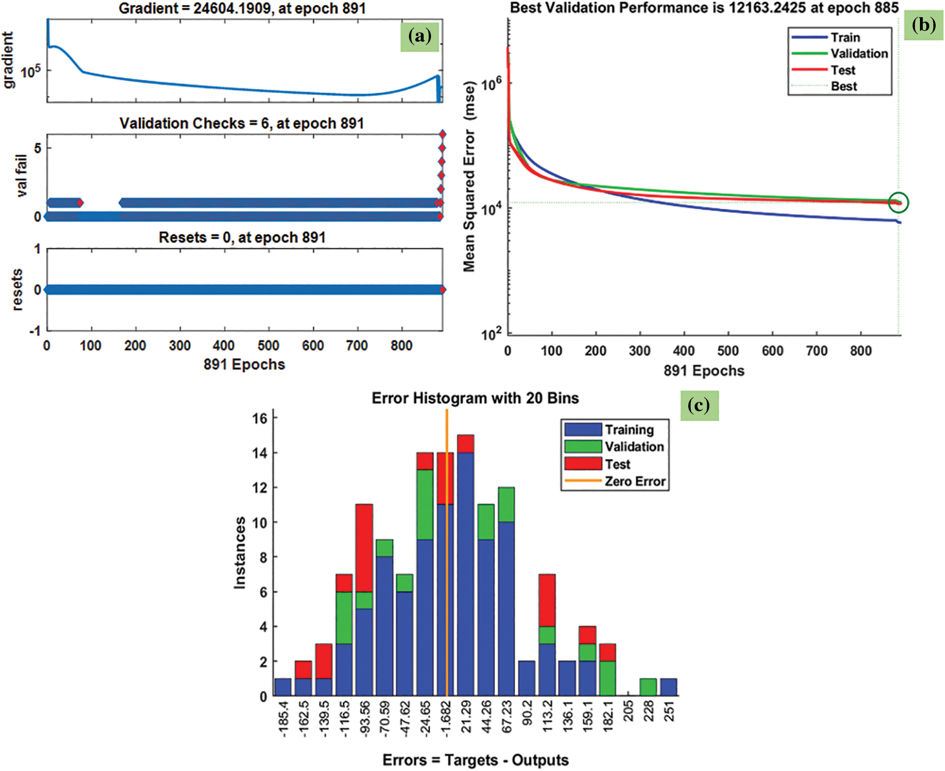
Figure 7: BFGS results of heat transfer coefficient: (a) training state plot, (b) best validation performance, and (c) error histogram

The R2 values of heat transfer predicted from the BFGS method are given in Fig. 8. The R2 for the training data is 0.99111 (Fig. 8a), R2 for the validation data is 0.98667 (Fig. 8b), R2 for the testing data is 0.98769 (Fig. 8c), and R2 for all the data is 0.98898 (Fig. 8d). The predicted data is almost approaching 1. The MSE, RMSE and R2 values of heat transfer predicted by the BFGS method are listed in Table 2.

Figure 8: BFGS results of R2 for heat transfer coefficient: (a) training, (b) validation, and (c) testing, and (d) all the data

Fig. 9 indicates the predicted heat transfer results using the VLGD method for the Fe3O4-SiO2 hybrid nanofluids. The training state plot, best validation performance, and error histogram are presented in Fig. 9a–c. From the figures, it can be observed that the gradient of the solution is 1548.8187 at epoch 102. This indicates that the solution converged very smoothly without disturbing the data. Under the same epoch of 102, the validation checks are 6 (Fig. 9a), and the Mu value is 10. The best validation performance is 7245.5869 as seen in Fig. 9b at epoch 126, and it clearly shows the merging of training, validation, testing, and the best performance meeting at epoch 126. The error histogram with 20 Bins is shown in Fig. 9c, where the error is −7.639, and is defined as the difference between targets and outputs.

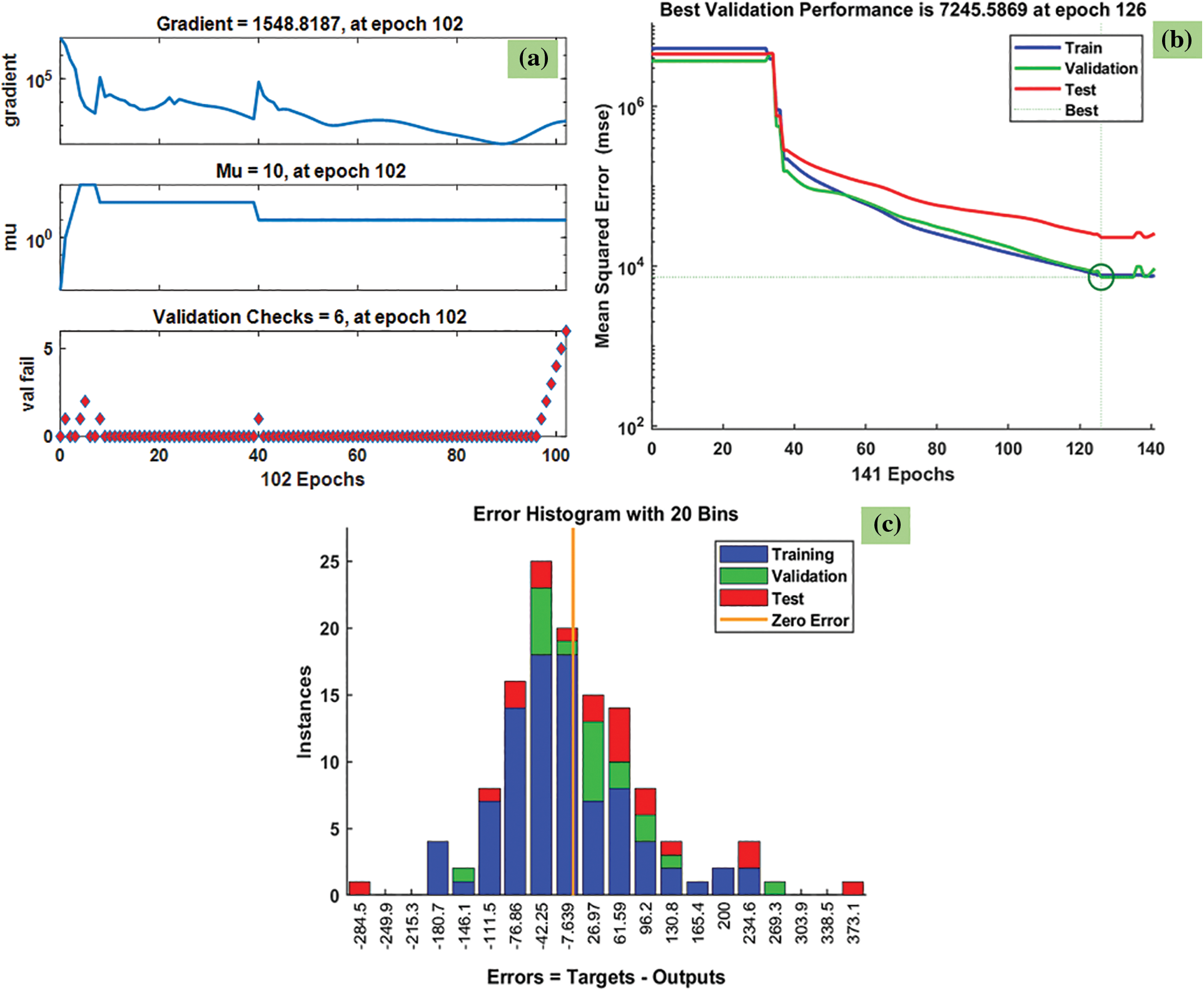
Figure 9: VLGD results of heat transfer coefficient: (a) training state plot, (b) best validation performance, and (c) error histogram

The R2 values of heat transfer predicted from the VLGD method are given in Fig. 10. The R2 for the training data is 0.98836 (Fig. 10a), R2 for the validation data is 0.99076 (Fig. 10b), R2 for test data is 0.97794 (Fig. 10c), and R2 for all the data is 0.98569 (Fig. 10d). The predicted data is almost approaching 1. The MSE, RMSE and R2 values of heat transfer predicted by the VLGD method are listed in Table 3. Three neural network methods were used to predict the heat transfer data and it was found that the LM method had superior predictability, when compared to the other two methods.

Figure 10: VLGD results of R2 for heat transfer coefficient: (a) training, (b) validation, and (c) testing, and (d) all the data

4.2 Nusselt Number

The back-propagation network contains four input parameters and one output parameter (Nusselt number) and those are connected by using hidden layers. There were 10 hidden layers and the weight and bias of each neuron in hidden layers are optimized using three algorithms and their results are compared. The network was trained with 70% of the data and tested and validated with 30% of the data.

Fig. 11 indicates the predicted Nusselt number data by the LM method for Fe3O4-TiO2 hybrid nanofluids. The training state plot, best validation performance, and error histogram are presented in Fig. 11a–c. From the figures, it can be observed that the gradient of the solution is 0.028463 at epoch 46. This indicates that the solution converged very smoothly without disturbing the data. Under the same epoch of 46, the validation checks are 6, and the Mu value is 0.0001 (Fig. 11a). The best validation performance is 0.023671 as seen in Fig. 11b at epoch 40; also, it clearly shows the merging of training, validation, testing, and the best performance meeting at epoch 40. The error histogram with 20 Bins is shown in Fig. 11c, and it indicates an error of −0.001916.

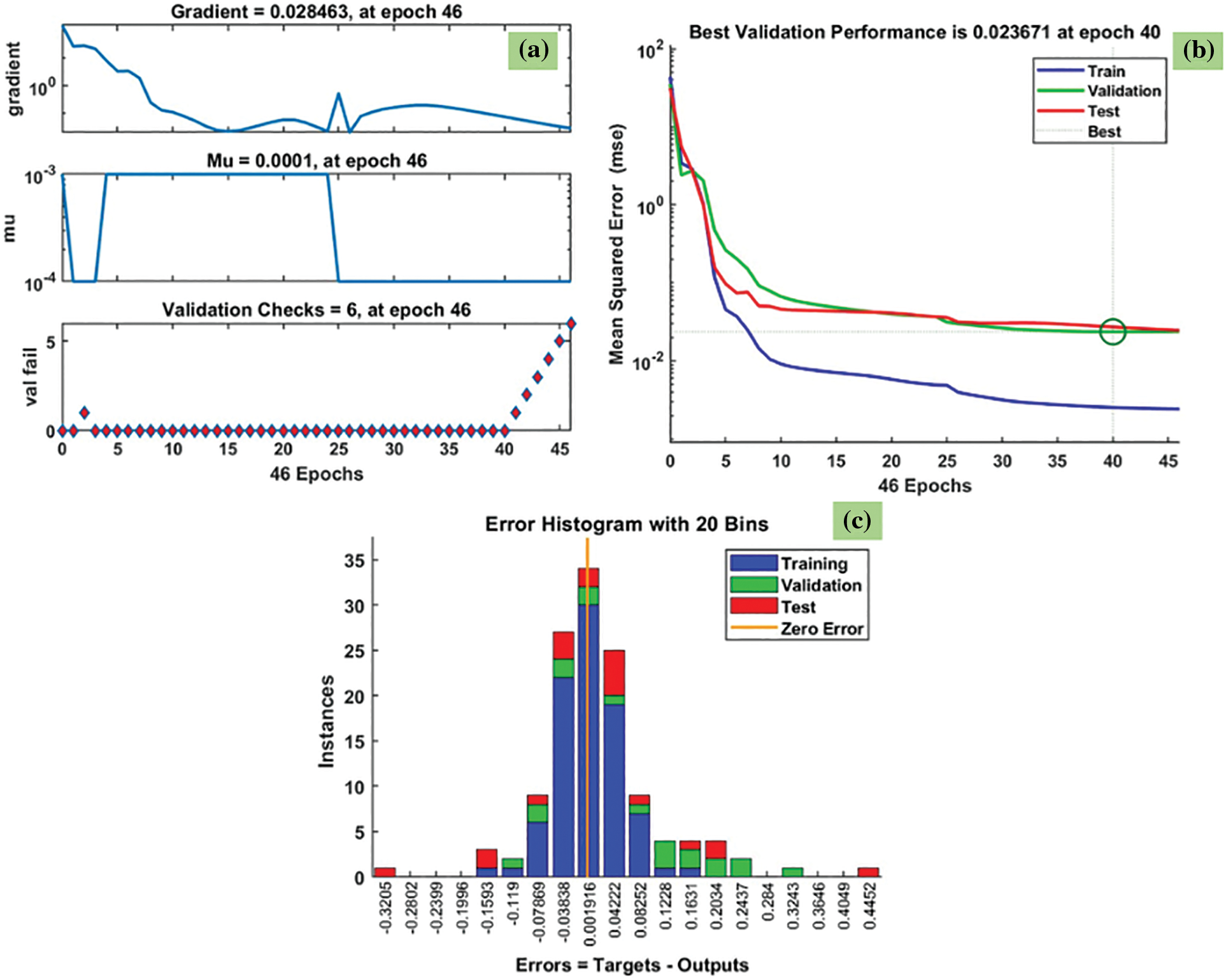
Figure 11: LM results of Nusselt results: (a) training state plot, (b) best validation performance, and (c) error histogram

The R2 values of heat transfer predicted from the LM method are given in Fig. 12. The R2 for the training data is 0.99986 (Fig. 12a), the R2 for the validation data is 0.9994 (Fig. 12b), the R2 for the testing data is 0.99883 (Fig. 12c), and R2 for all the data is 0.99954 (Fig. 12d). The predicted data is almost approaching 1. The MSE, RMSE and R2 values of the Nusselt number predicted by the LM method are listed in Table 4.

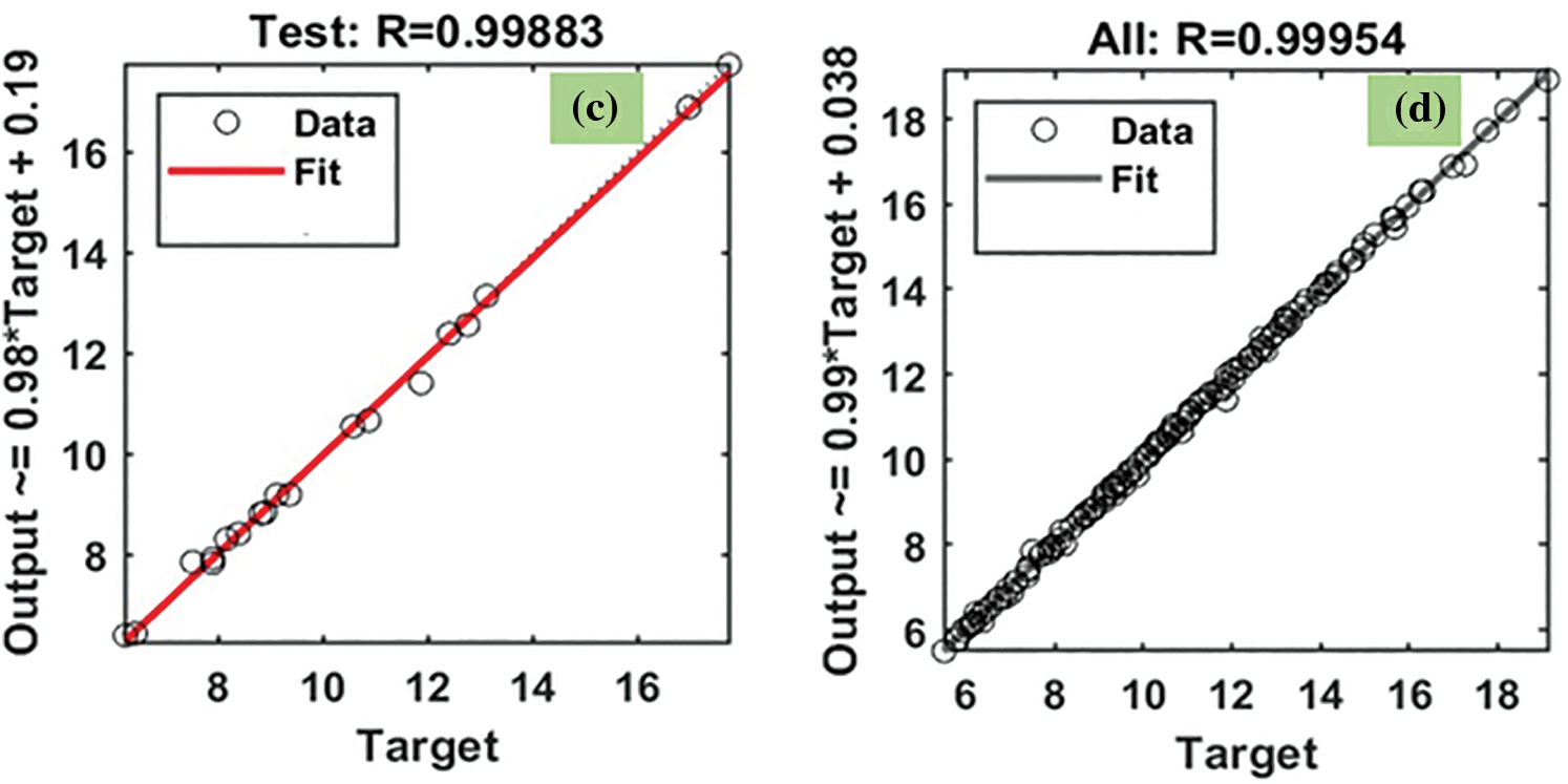
Figure 12: LM results of R2 for Nusselt number: (a) training, (b) validation, and (c) testing, and (d) all the data

Fig. 13 indicates the predicted Nusselt number data by the BFGS method for Fe3O4-TiO2 hybrid nanofluids. The training state plot, best validation performance, and error histogram are reported in Fig. 13a–c. From the figures, it can be observed that the gradient of the solution is 0.26311 at epoch 41. This indicates that the solution converged very smoothly without disturbing the data. Under the same epoch of 41, the validation checks are 6 (Fig. 13a). The best validation performance is 0.15048 as seen in Fig. 13b at epoch 35; it also shows the merging of training, validation, testing, and the best performance meeting this epoch. The error histogram with 20 Bins is shown in Fig. 13c, and it indicates an error of −0.02347.

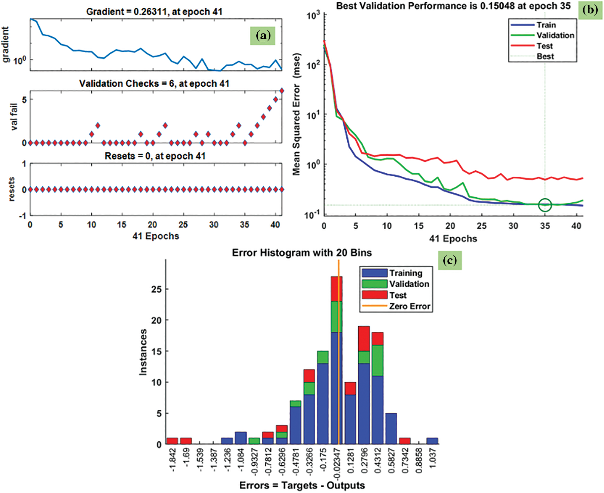
Figure 13: BFGS results of Nusselt number: (a) training state plot, (b) best validation performance, and (c) error histogram

The R2 values of heat transfer predicted by the BFGS method are given in Fig. 14. The R2 for the training data is 0.99637 (Fig. 14a), R2 for the validation data is 0.99666 (Fig. 14b), R2 for the testing data is 0.99739 (Fig. 14c), and R2 for all the data is 0.9967 (Fig. 14d). The predicted data is almost approaching 1. The MSE, RMSE and R2 values of the Nusselt number predicted by the BFGS method are listed in Table 5.

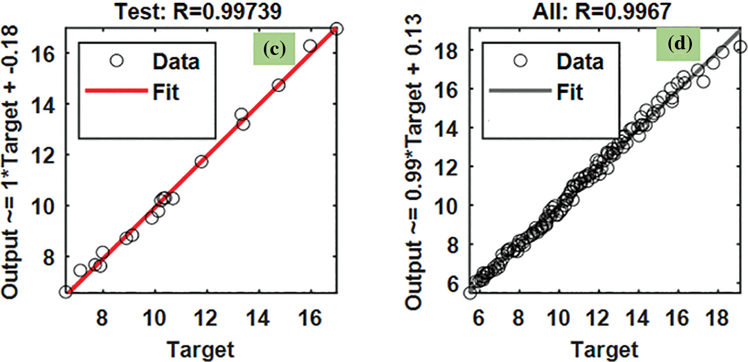
Figure 14: BFGS results of R2 for Nusselt number: (a) training, (b) validation, and (c) testing, and (d) all the data

Fig. 15 indicates the predicted Nusselt number data by the VLGD method for Fe3O4-TiO2 hybrid nanofluids. The training state plot, best validation performance, and error histogram are presented in Fig. 15a–c. From the figures, it can be observed that the gradient of the solution is 0.60196 at epoch 88. This indicates that the solution converged very smoothly without disturbing the data. Under the same epoch of 88, the validation checks are 6 (Fig. 15a). The best validation performance is 0.98756 as seen in Fig. 15b at epoch 82; it clearly shows the merging of training, validation, testing, and the best performance meeting at epoch 82. The error histogram with 20 Bins is shown in Fig. 15c, and it indicates an error of −0.0065.

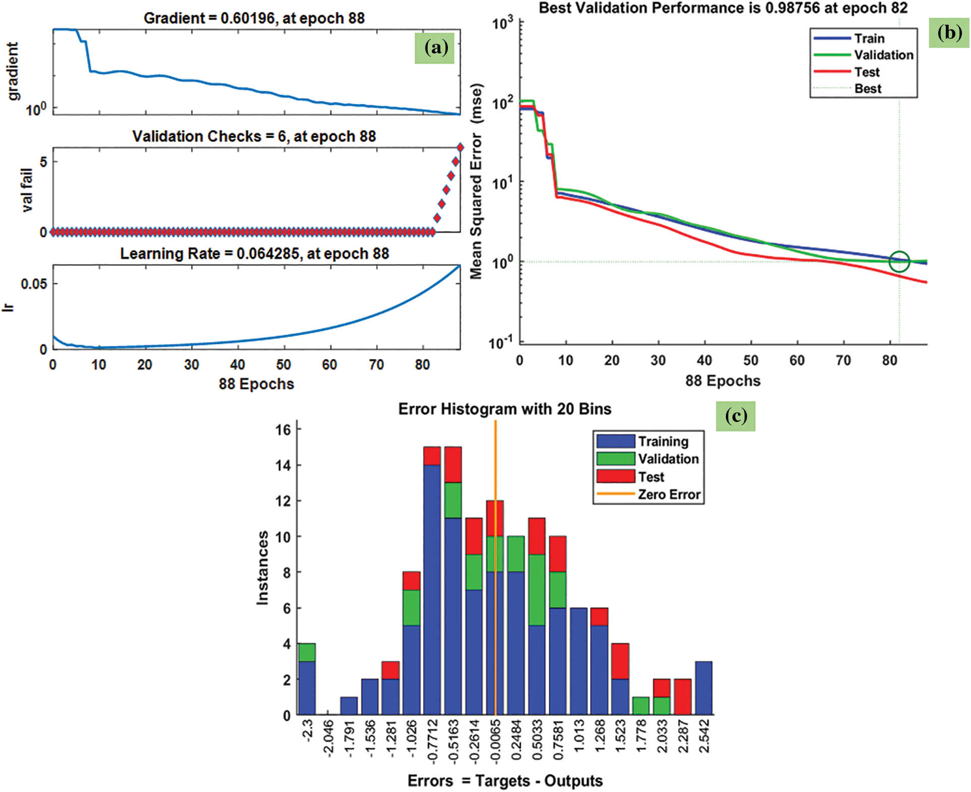
Figure 15: VLGD results of Nusselt number: (a) training state plot, (b) best validation performance, and (c) error histogram

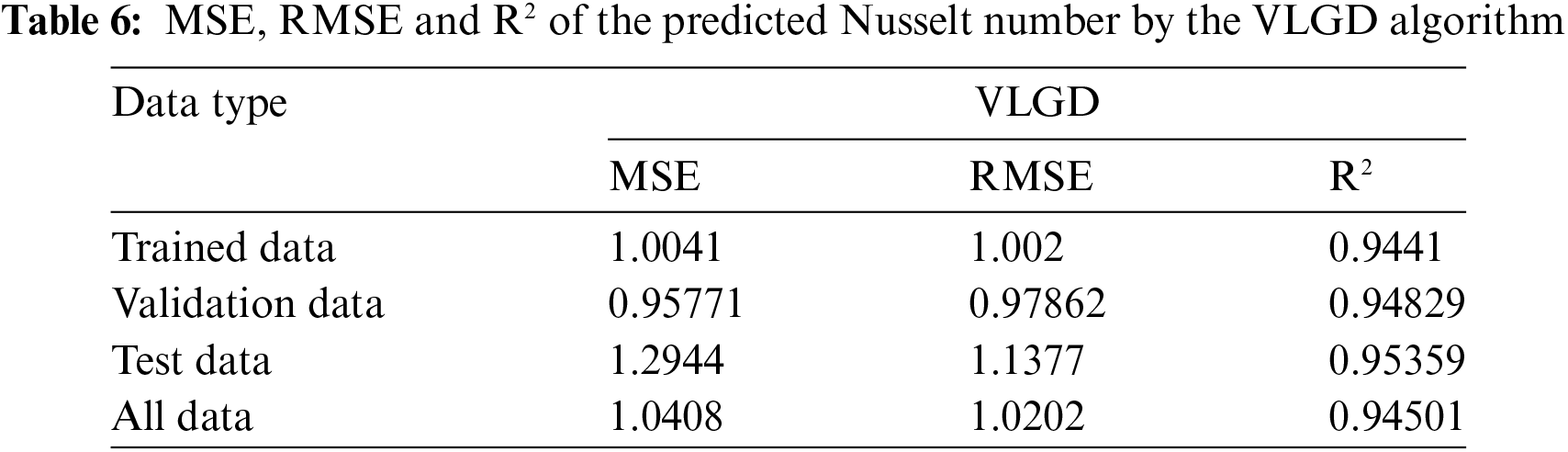
The R2 values of heat transfer predicted from the VLGD method are given in Fig. 16. The R2 for the training data is 0.9441 (Fig. 16a), R2 for the validation data is 0.94829 (Fig. 16b), R2 for the testing data is 0.95395 (Fig. 16c), and R2 for all the data is 0.94501 (Fig. 16d). The predicted data is almost approaching 1. The MSE, RMSE and R2 values of the Nusselt number predicted by the BFGS method are listed in Table 6.

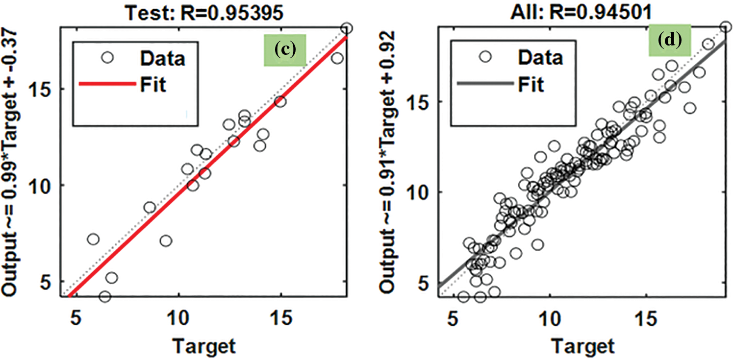
Figure 16: VLGD results of R2 for Nusselt number: (a) training, (b) validation, and (c) testing, and (d) all the data

From the predicted Nusselt number data, it can be noted that the LM and BFGS methods have good accuracy in predicting the experimental data, when compared to the VLGD method. The developed Nusselt number equation is given as follows.

(12)

The average deviation of Eq. (12) is 4.819%.

4.3 Friction Factor

The back-propagation network contains four input parameters and one output parameter (friction factor) and those are connected by using hidden layers. There were 10 hidden layers and the weight and bias of each neuron in hidden layers are optimized using three algorithms and their results are compared. The network was trained with 70% of the data and, tested and validated with 30% of the data.

Fig. 17 indicates the predicted friction factor data by the LM method for Fe3O4-TiO2 hybrid nanofluids. The training state plot, best validation performance, and error histogram are presented in Fig. 17a–c. From the figures, it can be observed that the gradient of the solution is 5.5142 × 10–5 at epoch 58. This indicates that the solution converged very smoothly without disturbing the data. Under the same epoch of 88, the validation checks are 6 (Fig. 17a) and the Mu value is 1 × 10–8. The best validation performance is 6.5761 × 10–6 as seen in Fig. 17b at epoch 52; also, it is clearly shown the merging of training, validation, testing, and the best performance meeting at epoch 52. The error histogram with 20 Bins is shown in Fig. 17c, and it indicates an error of −0.000207.

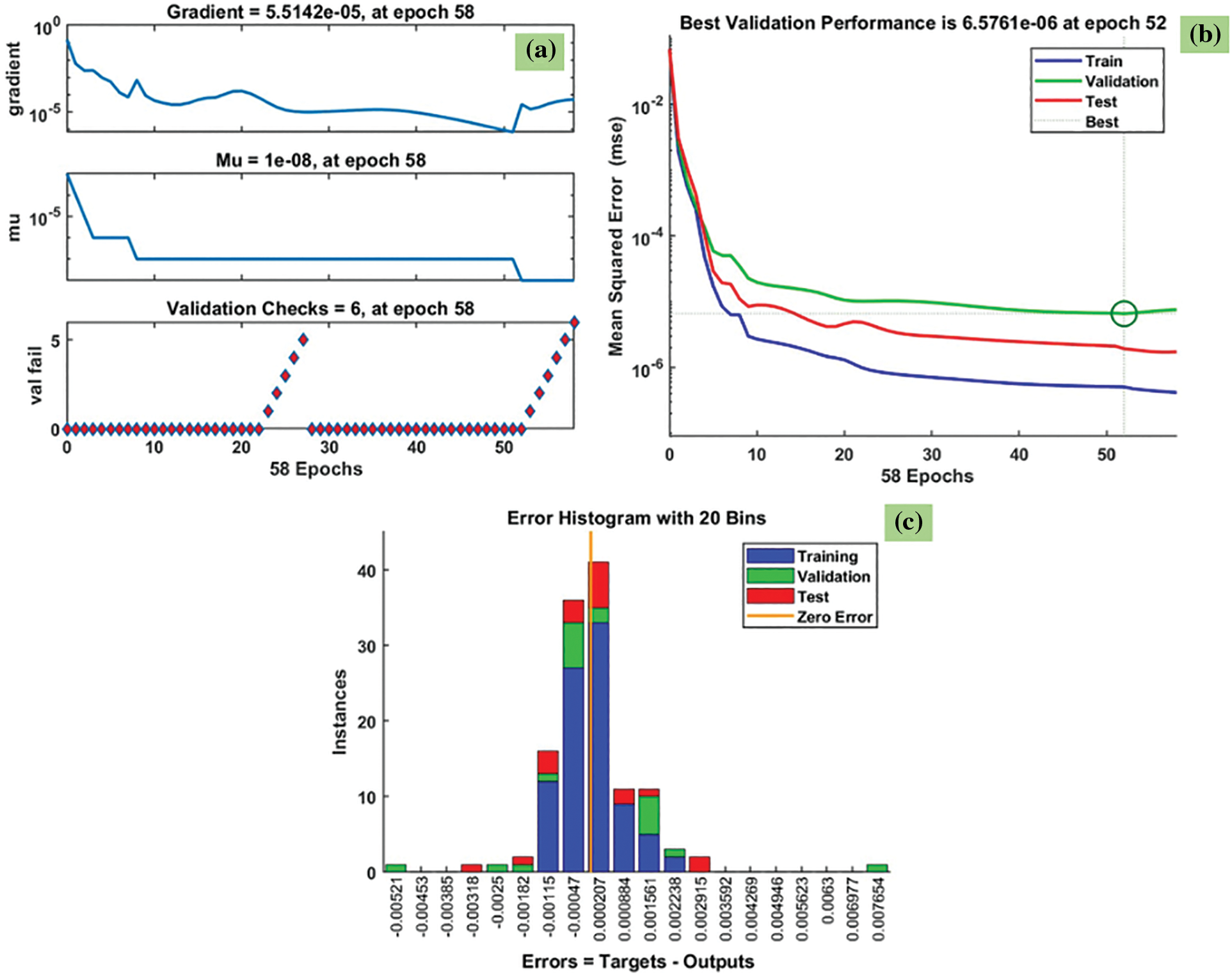
Figure 17: LM results of friction factor: (a) training state plot, (b) best validation performance, and (c) error histogram

The R2 values of heat transfer predicted from the LM method are given in Fig. 18. The R2 for the training data is 0.99993 (Fig. 18a), the R2 for the validation data is 0.99932 (Fig. 18b), the R2 for the testing data is 0.99987 (Fig. 18c), and R2 for all the data is 0.99982 (Fig. 18d). The predicted data is almost approaching 1. The MSE, RMSE and R2 values of the Nusselt number predicted by the BFGS method are listed in Table 7.

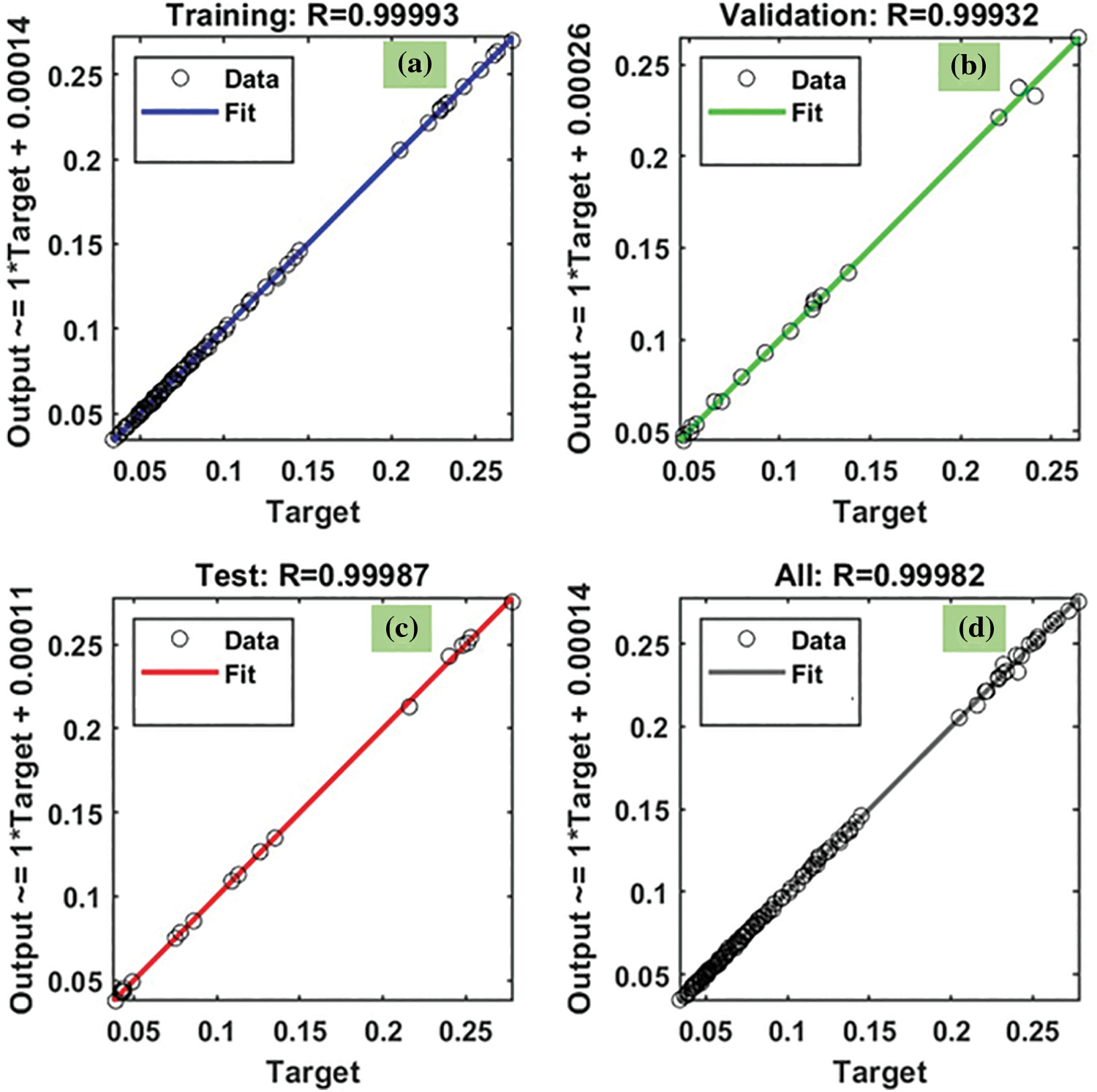
Figure 18: LM results of R2 for friction factor: (a) training, (b) validation, and (c) testing, and (d) all the data

Fig. 19 indicates the predicted friction factor data by the BFGS method for Fe3O4-TiO2 hybrid nanofluids. The training state plot, best validation performance, and error histogram are reported in Fig. 19a–c. From the figures, it can be observed that the gradient of the solution is 0.00035905 at epoch 47. This indicates that the solution converged very smoothly without disturbing the data. Under the same epoch of 47, the validation checks are 6 (Fig. 19a). The best validation performance is 2.3442 × 10–5 was seen in Fig. 19b at epoch 41; also, it shows the merging of training, validation, testing, and the best performance meeting at epoch 41. The error histogram with 20 Bins is shown in Fig. 19c, and it indicates an error of −0.00034.

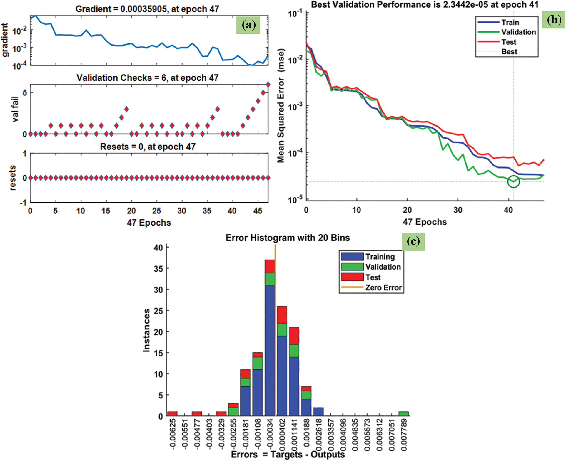
Figure 19: BFGS results of friction factor: (a) training state plot, (b) best validation performance, and (c) error histogram

The R2 values of heat transfer predicted from the BFGS method are given in Fig. 20. The R2 for the training data is 0.99991 (Fig. 20a), R2 for the validation data is 0.99874 (Fig. 20b), R2 for the testing data is 0.99961 (Fig. 20c), and R2 for all the data is 0.99976 (Fig. 20d). The predicted data is almost approaching 1. Table 8 lists the MSE, RMSE, and R2 values of the Nusselt number predicted by the BFGS method.

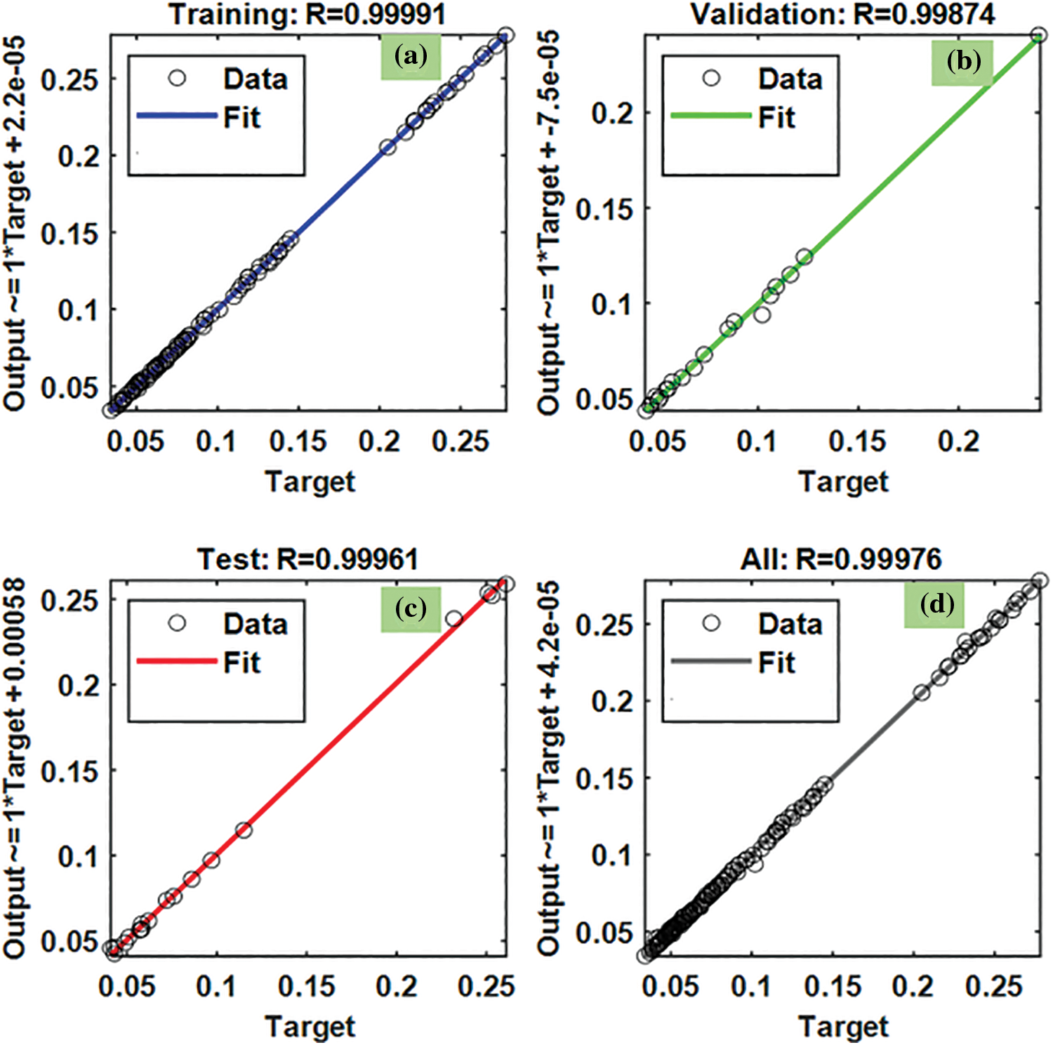
Figure 20: BFGS results of R2 for friction factor: (a) training, (b) validation, and (c) testing, and (d) all the data

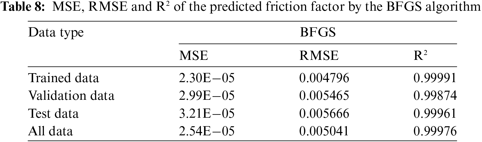
Fig. 21 indicates the predicted friction factor data by the VLGD method for Fe3O4-TiO2 hybrid nanofluids. The training state plot, best validation performance, and error histogram are presented in Fig. 21a–c. From the figures, it can be observed that the gradient of the solution is 0.00017646 at epoch 237. It indicates that the solution converged very smoothly without disturbing the data. Under the same epoch of 237, the validation check is 6 (Fig. 21a). The best validation performance of 5.8924 × 10–5 is seen in Fig. 21b at epoch 230; also, it clearly shows the merging of training, validation, and testing, and the best performance meeting at epoch 230. The error histogram with 20 Bins is shown in Fig. 21c, and it indicates an error of −0.0002.

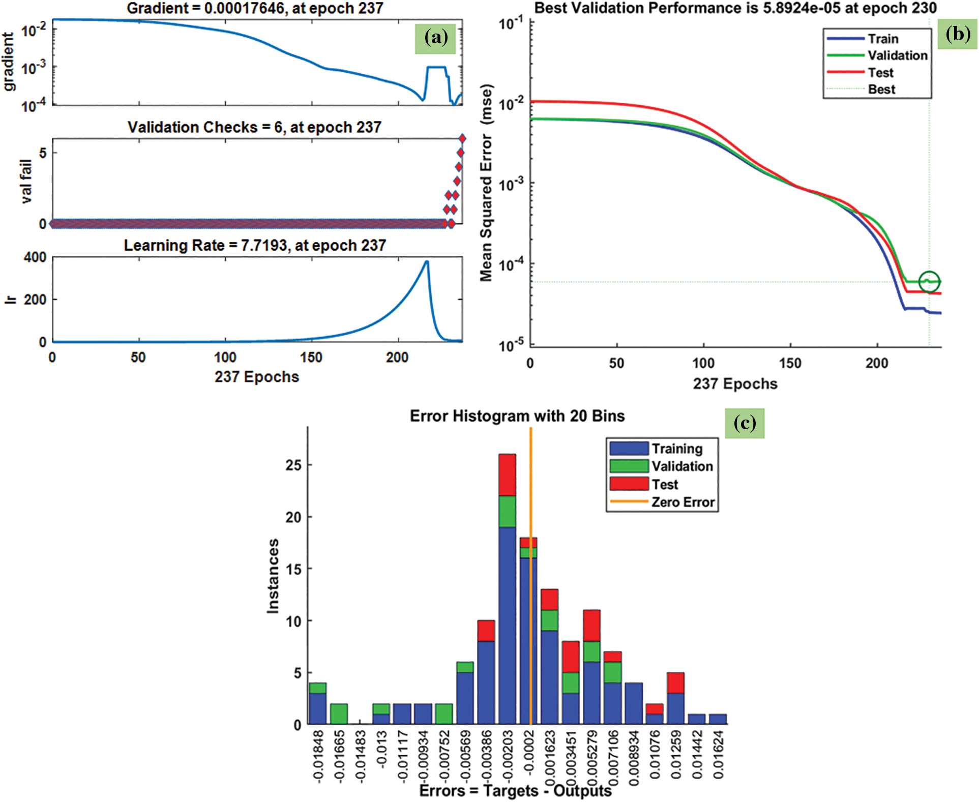
Figure 21: VLGD results of friction factor: (a) training state plot, (b) best validation performance, and (c) error histogram

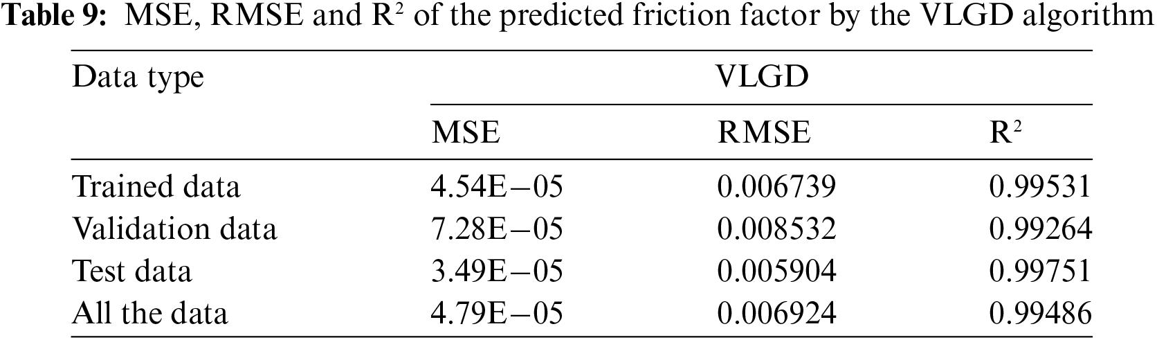
Table 2: values of heat transfer predicted by the VLGD method are given in Fig. 22. The R2 for the training data is 0.99531 (Fig. 22a), R2 for the validation data is 0.99264 (Fig. 22b), R2 for the testing data is 0.99751 (Fig. 22c), and R2 for all the data is 0.99486 (Fig. 22d). The predicted data is almost approaching 1. The MSE, RMSE and R2 values of the Nusselt number predicted by the BFGS method are listed in Table 9.

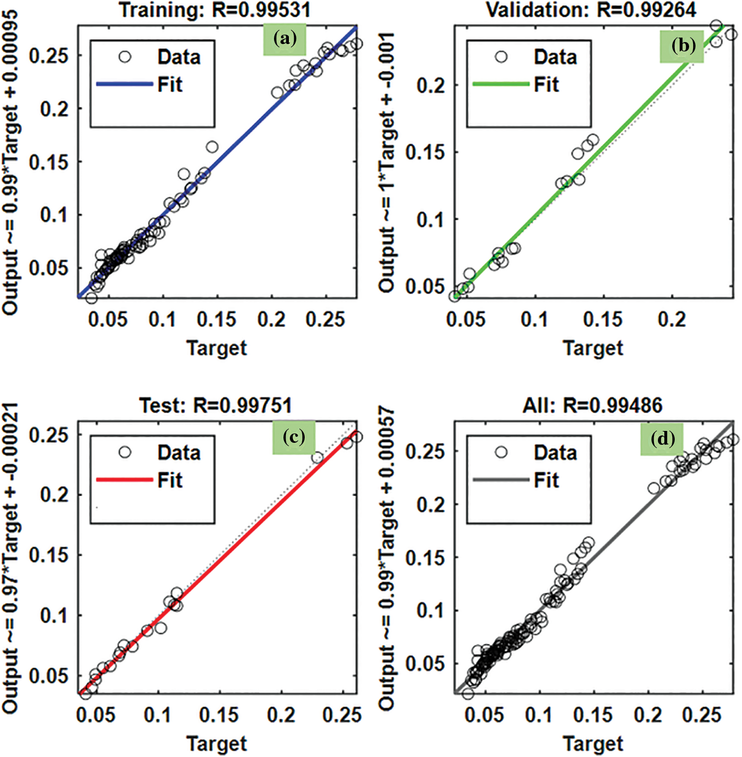
Figure 22: VLGD results of R2 for friction factor: (a) training, (b) validation, and (c) testing, and (d) all the data

The developed friction factor equation is as follows:

(13)

The average deviation of Eq. (13) is 5.685%.

4.4 ANOVA t-Test Analysis

In the present study, three algorithms were used to predict the heat transfer, Nusselt number, and friction factor data. The best algorithm was analyzed using ANOVA and t-test. Initially ANOVA is used to compare three models. If a significant difference is found using ANOVA, a t-test is evaluated for LM vs. BFGS, LM vs. VLGD, and BFGS vs. VLGD to find the best algorithm. The ANOVA analysis is performed using MSE and RMSE results for all training, testing, and validation datasets. The ANOVA analysis suggested that the F-statistic is 64.7178526, with a corresponding p-value of 1.05E−09 for the Nusselt number. The p-value (1.05 × 10–9) is lower than the significance level of 0.05. Since the p-value is lower than the significance level, we can reject the null hypothesis and conclude that there is a statistically significant difference in the means of the dependent variable among the three groups. Hence, the t-test analysis was conducted between LM vs. BFGS, LM vs. VLGD, and BFGS vs. VLGD, and finally, draw the best algorithm based on the p-value.

Table 10 suggests that the one-tailed p-value (= 0.036238) is less than the significance level of 0.05 for LM vs., BFGS in comparison to LM vs. VLGD and BFGS vs. VLGD. There is a statistically significant difference between the means of LM and BFGS, with the mean of LM being lower than the mean of BFGS. Based on the t-test analyses, the best-performing method appears to be VLGD, as it has the highest mean among the three methods and there is no statistically significant difference between its mean and the means of the other two methods (LM and BFGS). The analysis suggests that the VLGD method outperforms the LM method, as the mean of VLGD is significantly higher than the mean of LM. However, the BFGS method also performs well, as its mean value is not significantly different from that of VLGD.

Table 11 suggests that the one-tailed p-value for LM vs. VLGD and BFGS vs. VLGD is lower than the significance level of 0.05. The LM and BFGS methods do not have a statistically significant difference in their means, suggesting they perform similarly. The best-performing method appears to be VLGD, as it has a significantly higher mean compared to both LM and BFGS, and the differences are statistically significant.

Table 12 shows that p-value is lower for LM vs. VLGD and BFGS vs. VLGD. There is a significant difference between LM and VLGD as well as BFGS and VLGD. The best-performing method appears to be VLGD, as it has a significantly higher mean compared to both LM and BFGS, and the differences are statistically significant.

5  Conclusions

The backpropagation artificial neural network (ANN) methods of Levenberg-Marquardt (LM), Broyden-Fletcher-Goldfarb-Shanno Quasi-Newton (BFGS), and Variable Learning Rate Gradient Descent (VLGD) were used to predict the experimental data. The heat transfer, Nusselt number, and friction factor data of water-based Fe3O4-TiO2 magnetic hybrid nanofluids in a mini-heat sink were considered for the analysis. The data selected as network input data is Reynolds number (range from 239 to 1874), volume concentration (range from 0% to 2%), and magnetic field (range from 250 to 1000 G). In this study, a total of 126 datasets were used. The ANOVA t-test analysis was also performed to understand the best ANN algorithm among the three networks. The main findings of the study are:

•   The results given by the LM, BFGS, and VLGD algorithms for the heat transfer coefficient indicate that: the MSE is 8.47 × 102, 7.34 × 103, and 9859.21, respectively, the RMSE is 29.1083, 87.40, and 99.29, respectively, and the R2 value is 0.99968, 0.98898, and 0.98569, respectively.

•   The results given by the LM, BFGS, and VLGD algorithms for the Nusselt number indicate that: the MSE is 0.12168, 0.64216, and 1.0408, respectively, the RMSE is 0.34883, 0.25341, and 1.0202, respectively, and the R2 value is 0.99954, 0.9967, and 0.94501, respectively.

•   The results given by the LM, BFGS, and VLGD algorithms for the friction factor indicate that: the MSE is 2.21 × 10–6, 2.54 × 10–5, and 4.79 × 10–5, respectively, the RMSE is 0.001488, 0.005041, and 0.006924, respectively, and the R2 value is 0.99982, 0.99976, and 0.99486, respectively.

•   The LM algorithm predicts the data with high accuracy compared to the other two methods.

•   The ANOVA t-test also shown, the LM method is the best method to predict the data, as compared to the other two methods.

•   By using the LM algorithm, polynomial regression equations were developed for the Nusselt number and friction factor.

The study indicates that the ANN algorithms, in general, and particularly the LM algorithm, are outstanding tools to provide for further understanding of the experimental data trend.

Acknowledgement: This work is supported by the Recovery and Resilience Plan (PRR) and by European Funds Next Generation EU under the Project “AET—Alliance for Energy Transition,” no. C644914747-00000023, investment project no. 56 of the Incentive System “Agendas for Business Innovation”.

Funding Statement: The authors received no specific funding for this study.

Author Contributions: The authors confirm their contribution to the paper as follows: L. S. Sundar: data analysis, comparison of the data and initial draft writing; Sérgio M. O. Tavares: study conception and design; António M. B. Pereira: data collection; Antonio C. M. Sousa: analysis and interpretation of results. All authors reviewed the results and approved the manuscript in its present version.

Availability of Data and Materials: There is no unavailable data in this study.

Ethics Approval: Not applicable.

Conflicts of Interest: The authors declare no conflicts of interest to report regarding the present study.

References

1. Choi SUS, Eastman JA. Enhancing thermal conductivity of fluids with nanoparticles. In: 1995 International Mechanical Engineering Congress and Exhibition; 1995; San Francisco, CA, USA. [Google Scholar]

2. Moghaddam MA, Motahari K, Rezaei A. Performance characteristics of low concentrations of CuO/water nanofluid flowing through horizontal tube for energy efficiency purposes: an experimental study and ANN modeling. J Mol Liq. 2018;271:342–52. doi:10.1016/j.molliq.2018.08.149. [Google Scholar] [CrossRef]

3. Madhesh D, Parameshwaran R, Kalaiselvam S. Experimental studies on convective heat transfer and pressure drop characteristics of metal and metal-oxide nanofluids under turbulent flow regime. Heat Transf. 2016;37:422–34. doi:10.1080/01457632.2015.1057448. [Google Scholar] [CrossRef]

4. Hussein AM, Bakar RA, Kadirgama K. Study of forced convection nanofluid heat transfer in the automotive cooling system. Case Stud Therm Eng. 2014;2:50–61. doi:10.1016/j.csite.2013.12.001. [Google Scholar] [CrossRef]

5. Ardekani AM, Kalantar V, Heyhat MM. Experimental study on heat transfer enhancement of nanofluid flow through helical tubes. Adv Powder Technol. 2019;30:1815–22. doi:10.1016/j.apt.2019.05.026. [Google Scholar] [CrossRef]

6. Sundar LS, Abebaw HM, Singh MK, Pereira AMB, Sousa ACM. Experimental heat transfer and friction factor of Fe3O4 magnetic nanofluids flow in a tube under laminar flow at high Prandtl numbers. Int J Heat Technol. 2020;38:301–13. doi:10.18280/ijht.380204. [Google Scholar] [CrossRef]

7. Kumar V, Sarkar J. Numerical and experimental investigations on heat transfer and pressure drop characteristics of Al2O3-TiO2 hybrid nanofluid in mini-channel heat sink with different mixture ratio. Powder Technol. 2019;345:717–27. doi:10.1016/j.powtec.2019.01.061. [Google Scholar] [CrossRef]

8. Kumar V, Sarkar J. Two-phase numerical simulation of hybrid nanofluid heat transfer in minichannel heat sink and experimental validation. Int Commun Heat Mass Transf. 2018;91:239–47. doi:10.1016/j.icheatmasstransfer.2017.12.019. [Google Scholar] [CrossRef]

9. Ahammed N, Asirvatham LG, Wongwises S. Entropy generation analysis of graphene-alumina hybrid nanofluid in multiport minichannel heat exchanger coupled with thermoelectric cooler. Int J Heat Mass Transf. 2016;103:1084–97. doi:10.1016/j.ijheatmasstransfer.2016.07.070. [Google Scholar] [CrossRef]

10. Nimmagadda R, Venkatasubbaiah K. Conjugate heat transfer analysis of microchannel using novel hybrid nanofluids (Al2O3+Ag/water). Eur J Mech B/Fluids. 2015;52:19–27. doi:10.1016/j.euromechflu.2015.01.007. [Google Scholar] [CrossRef]

11. Nimmagadda R, Venkatasubbaiah K. Experimental and multiphase analysis of nanofluids on the conjugate performance of micro-channel at low Reynolds numbers. Heat Mass Transf. 2017;53:2099–115. doi:10.1007/s00231-017-1970-2. [Google Scholar] [CrossRef]

12. Nanda Kishore PVR, Venkatachalapathy S, Kalidoss P. Experimental investigation on thermohydraulic performance of hybrid nanofluids in a novel minichannel heat sink. Thermochim Acta. 2023;721:179452. doi:10.1016/j.tca.2023.179452. [Google Scholar] [CrossRef]

13. Murali Krishna V, Sandeep Kumar M, Muthalagu R, Senthil Kumar P, Mounika R. Numerical study of fluid flow and heat transfer for flow of Cu-Al2O3-water hybrid nanofluid in a microchannel heat sink. Mater Today: Proc. 2022;49(5):1298–302. doi:10.1016/j.matpr.2021.06.385. [Google Scholar] [CrossRef]

14. Santra AK, Chakraborty N, Sen S. Prediction of heat transfer due to presence of copper-water nanofluid using resilient-propagation neural network. Int J Therm Sci. 2009;48:1311–8. doi:10.1016/j.ijthermalsci.2008.11.009. [Google Scholar] [CrossRef]

15. Balcilar M, Dalkilic AS, Suriyawong A, Yiamsawas T, Wongwises S. Investigation of pool boiling of nanofluids using artificial neural networks and correlation development techniques. Int Commun Heat Mass Transf. 2012;39:424–31. doi:10.1016/j.icheatmasstransfer.2012.01.008. [Google Scholar] [CrossRef]

16. Bahiraei M, Hangi M. Investigating the efficacy of magnetic nanofluid as a coolant in double-pipe heat exchanger in the presence of magnetic field. Energy Convers Manag. 2013;76:1125–33. doi:10.1016/j.enconman.2013.09.008. [Google Scholar] [CrossRef]

17. Naphon P, Wiriyasart S, Arisariyawong T, Nakharintr L. ANN, numerical and experimental analysis on the jet impingement nanofluids flow and heat transfer characteristics in the micro-channel heat sink. Int J Heat Mass Transf. 2019;131:329–40. doi:10.1016/j.ijheatmasstransfer.2018.11.073. [Google Scholar] [CrossRef]

18. Tafarroj MM, Mahian O, Kasaeian A, Sakamatapan K, Dalkilic AS, Wongwises S. Artificial neural network modeling of nanofluid flow in a microchannel heat sink using experimental data. Int Commun Heat Mass Transf. 2017;86(3):25–31. doi:10.1016/j.icheatmasstransfer.2017.05.020. [Google Scholar] [CrossRef]

19. Khosravi R, Teymourtash AR, Fard MP, Rabiei S, Bahiraei M. Numerical study and optimization of thermohydraulic characteristics of a graphene-platinum nanofluid in finned annulus using genetic algorithm combined with decision-making technique. Eng Comput. 2021;37(3):2473–91. doi:10.1007/s00366-020-01178-6. [Google Scholar] [CrossRef]

20. Esfe MH. Designing a neural network for predicting the heat transfer and pressure drop characteristics of Ag/water nanofluids in a heat exchanger. Appl Therm Eng. 2017;126:559–65. doi:10.1016/j.applthermaleng.2017.06.046. [Google Scholar] [CrossRef]

21. Yasir M, Khan M. Dynamics of unsteady axisymmetric of Oldroyd-B material with homogeneous-heterogeneous reactions subject to Cattaneo-Christov heat transfer. Alex Eng J. 2023;74:665–74. doi:10.1016/j.aej.2023.05.065. [Google Scholar] [CrossRef]

22. Yasir M, Khan M, Hussain SM, Khan H, Saleem S. Numerical aggregation for dissipative flow of hybrid nanomaterial: darcy Forchheimer model. Ain Shams Eng J. 2024;15:102628. doi:10.1016/j.asej.2024.102628. [Google Scholar] [CrossRef]

23. Ghofrani A, Dibaei MH, Hakim Sima A, Shafii MB. Experimental investigation on laminar forced convection heat transfer of ferrofluids under an alternating magnetic field. Exp Therm Fluid Sci. 2013;49:193–200. doi:10.1016/j.expthermflusci.2013.04.018. [Google Scholar] [CrossRef]

24. Ashjaee M, Goharkhah M, Khadem LA, Ahmadi R. Effect of magnetic field on the forced convection heat transfer and pressure drop of a magnetic nanofluid in a miniature heat sink. Heat Mass Transf. 2015;51(7):953–64. doi:10.1007/s00231-014-1467-1. [Google Scholar] [CrossRef]

25. Riaz Khan M, Li M, Mao S, Ali R, Khan S. Comparative study on heat transfer and friction drag in the flow of various hybrid nanofluids effected by aligned magnetic field and nonlinear radiation. Sci Rep. 2021;11:3691. doi:10.1038/s41598-021-81581-1. [Google Scholar] [PubMed] [CrossRef]

26. Tekir M, Taskesen E, Gedik E, Arslan K, Aksu B. Effect of constant magnetic field on Fe3O4-Cu/water hybrid nanofluid flow in a circular pipe. Heat Transf Eng. 2021;58:707–17. doi:10.1007/s00231-021-03125-7. [Google Scholar] [CrossRef]

27. Alsarraf J, Rahmani R, Shahsavar A, Afrand M, Wongwises S, Tran MD. Effect of magnetic field on laminar forced convective heat transfer of MWCNT-Fe3O4/water hybrid nanofluid in a heated tube. J Therm Anal Calorim. 2019;137:1809–25. doi:10.1007/s10973-019-08078-y. [Google Scholar] [CrossRef]

28. Mehrali M, Sadeghinezhad E, Akhiani AR, Latibari ST, Metselaar HSC, Kherbeet AS, et al. Heat transfer and entropy generation analysis of hybrid graphene/Fe3O4 ferro-nanofluid flow under the influence of a magnetic field. Powder Technol. 2017;308:149–57. doi:10.1016/j.powtec.2016.12.024. [Google Scholar] [CrossRef]

29. Sundar LS, Alklaibi AM, Sambasivam S, Mouli KVCC. Experimentally determining the thermophysical properties. Heat transfer and friction factor Fe3O4-TiO2 magnetic hybrid nanofluids in a mini-heat sink under magnetic field: proposing new correlations. J Magn Magn Mater. 2024;594:171889. doi:10.1016/j.jmmm.2024.171889. [Google Scholar] [CrossRef]