 Open Access
ARTICLE
Air-Side Heat Transfer Performance Prediction for Microchannel Heat Exchangers Using Data-Driven Models with Dimensionless Numbers
1 Institute of Process Equipment, College of Energy Engineering, Zhejiang University, Hangzhou, 310027, China
2 Institute of Wenzhou, Zhejiang University, Wenzhou, 310027, China
3 School of Intelligent Manufacturing Ecosystem, Xi’an Jiaotong-Liverpool University, Suzhou, 215123, China
* Corresponding Author: Long Huang. Email:
Frontiers in Heat and Mass Transfer 2024, 22(6), 1613-1643. https://doi.org/10.32604/fhmt.2024.058231
Received 07 September 2024; Accepted 16 October 2024; Issue published 19 December 2024
Abstract
This study explores the effectiveness of machine learning models in predicting the air-side performance of microchannel heat exchangers. The data were generated by experimentally validated Computational Fluid Dynamics (CFD) simulations of air-to-water microchannel heat exchangers. A distinctive aspect of this research is the comparative analysis of four diverse machine learning algorithms: Artificial Neural Networks (ANN), Support Vector Machines (SVM), Random Forest (RF), and Gaussian Process Regression (GPR). These models are adeptly applied to predict air-side heat transfer performance with high precision, with ANN and GPR exhibiting notably superior accuracy. Additionally, this research further delves into the influence of both geometric and operational parameters—including louvered angle, fin height, fin spacing, air inlet temperature, velocity, and tube temperature—on model performance. Moreover, it innovatively incorporates dimensionless numbers such as aspect ratio, fin height-to-spacing ratio, Reynolds number, Nusselt number, normalized air inlet temperature, temperature difference, and louvered angle into the input variables. This strategic inclusion significantly refines the predictive capabilities of the models by establishing a robust analytical framework supported by the CFD-generated database. The results show the enhanced prediction accuracy achieved by integrating dimensionless numbers, highlighting the effectiveness of data-driven approaches in precisely forecasting heat exchanger performance. This advancement is pivotal for the geometric optimization of heat exchangers, illustrating the considerable potential of integrating sophisticated modeling techniques with traditional engineering metrics.Keywords
Nomenclature
| A | Cross-sectional area |
| Ar | Aspect ratio |
| Bond number | |
| Boiling number | |
| Capillary number | |
| Convection number | |
| D | Depth (m) |
| Body force per unit mass (m/s2) | |
| Fr | Froude number |
| Galileo number | |
| H | Height (mm) |
| h | Height difference factor or geometric factor |
| HTC | Heat transfer coefficient (W/(m2·K)) |
| Hyd | Hydraulic diameter (m) |
| Jakob number | |
| Kapitza number | |
| L | Length (m) |
| LMTD | Logarithmic mean temperature difference (°C) |
| ṁ | Mass flow rate (kg/s) |
| m | Parameter (m) |
| N | Number of channels |
| Nu | Nusselt number |
| Pressure (Pa) | |
| Pressure at cold inlet | |
| Pressure at hot inlet | |
| Cold fluid Pressure drop | |
| Hot fluid Pressure drop | |
| Q | Heat transfer rate (W) |
| R | Thermal resistance (K/W) |
| Rd | Phases’ density ratio |
| Re | Reynolds number |
| S | Fin spacing (mm) |
| Sc | Schmidt number |
| Su | Suratman number |
| t | Thickness (m) |
| T | Temperature (°C) |
| Temperature at inlet of cold fluid | |
| Temperature at inlet of hot fluid | |
| Velocity (m/s) | |
| We | Weber number |
| Adaptive Neuro Fuzzy Interface System | |
| Artificial Neural Network | |
| Correlated-Informed Neural Networks | |
| Finite Element Method | |
| Finite Volume Method | |
| Gradient Boosting Machine | |
| Gaussian Process Regression | |
| Hybrid Radial Basis Function | |
| Radial Basis Function | |
| Random Forest | |
| Support Vector Machine | |
| Support Vector Regression | |
| Greek Characters | |
| Dynamic viscosity (Pa·s) | |
| Density (kg/m3) | |
| The differences | |
| Angle (°) | |
| Efficiency | |
| Viscous stress tensor (Pa) | |
| Subscripts | |
| Inlet | |
| Outlet | |
In recent decades, the global energy production has shifted from fossil fuels to renewable and low-carbon sources, notably in nuclear, wind, and solar sectors. This transition highlights the crucial role of efficient thermal management systems in ensuring the performance and safety of electronic devices, nuclear reactors, and industrial processes [1]. Heat exchanger finds applications in various industries, including air-conditioning, refrigeration, power generation, oil refining, petrochemical production, natural gas processing, chemical manufacturing, and sewage treatment, etc. [2,3]. Microchannel heat exchangers are pivotal in modern thermal management systems due to their high efficiency and lower refrigerant charge [4].
For microchannel heat exchangers, key performance indices include pressure drop and heat transfer rate. Pressure drop indicates the resistance fluids encounter within the exchanger, directly influencing the system’s energy efficiency and operational costs. Effective optimization of these parameters necessitates meticulous analysis and forecasting of the heat exchanger’s design. Traditional approaches primarily focus on experimental measurements and theoretical predictions based on simplified physical models, with Computational Fluid Dynamics (CFD) increasingly used to simulate detailed thermal behaviors.
Current approaches in predicting heat exchanger performance include theoretic models, numerical methods, and experiment methods have been commonly applied. Theoretic models typically simplify equations through specific assumptions to derive exact solutions. Numerical modeling employs techniques like the Finite Volume Method (FVM) or Finite Element Method (FEM) to discretize the refrigerant’s flow field and ensure heat and mass balance [5]. There are experiment methods that simulate the actual operating conditions and involve constructing prototypes [6]. Common methods to assess heat transfer include the Logarithmic Mean Enthalpy Difference (LMHD) [7] and Logarithmic Mean Temperature Difference (LMTD), which rely on assumptions of constant physical properties and continuous operation [8]. CFD discretizes the calculation domain to allow a generalized approach in tackling various fluid flow problems, though it requires substantial computational power [9].
Recently, Machine Learning (ML) has shown promise as an effective approach in the analysis of heat exchangers. Fig. 1 illustrates an increasing number of studies in this area showcasing the growing significance of ML methodologies applied in the domain of microchannel heat exchanger. Techniques like Artificial Neural Networks (ANN) [10], Support Vector Machines (SVM) [11], and Tree models [12] have proven successful in forecasting the performance of heat exchangers.
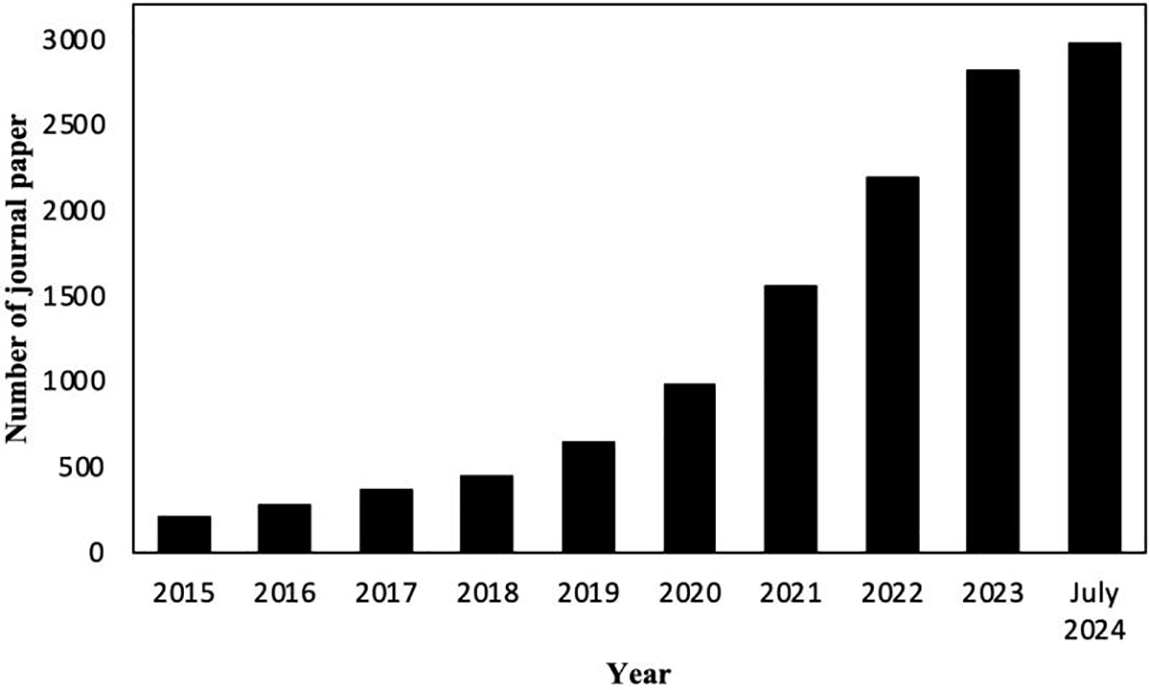
Figure 1: The trend in ML application to heat exchanger analysis from 2015 to July 2024 (based on ScienceDirect data) [13]
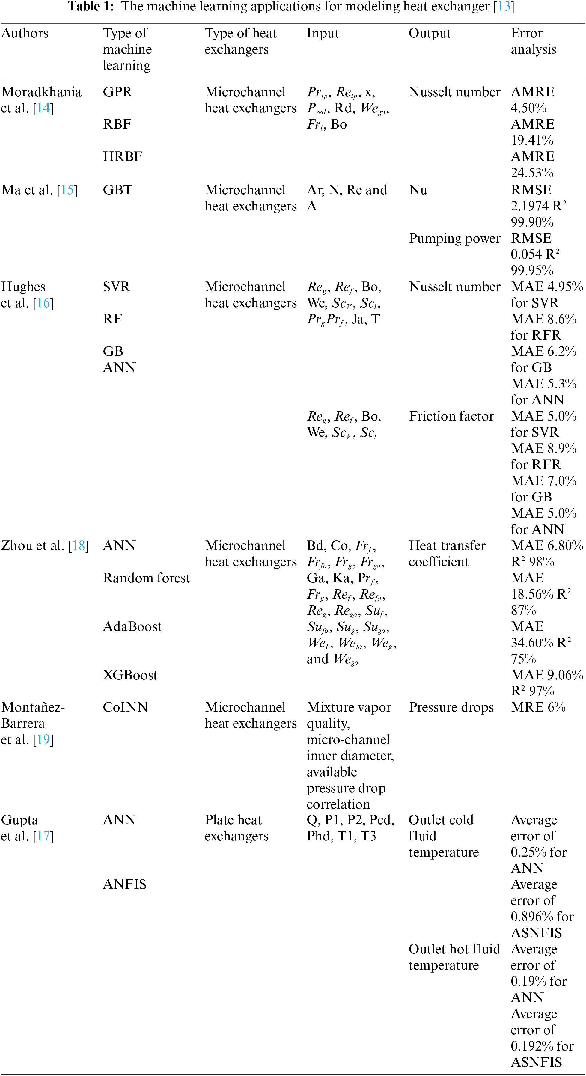
As indicated in Table 1, recent machine learning models applied to microchannel heat exchanger modeling predominantly focus on the performance of the refrigerant side given the large amount of refrigerant side testing data on heat transfer and pressure drop. Moradkhania et al. [14–16] have utilized machine learning models to model the tube-side of microchannel heat exchangers based on various dimensionless parameters and operational conditions. As the tube extraction techniques became more readily available, researchers can expect further data sets available on refrigerant-side, therefore allowing further enhancement of ML-based modeling for refrigerant flows. The prototyping and manufacturing process of a new fin design typically require a set of new set mold, fin mills and full heat exchanger assembly in order to test air-side performance data. This has resulted in limited experimental data available on different fin designs. Gupta et al. [17] explored machine learning modeling of air-side fin structures for plate heat exchanger with 24 data points, not including geometric information as input variables.
Despite the extensive application of CFD and traditional theoretical models in predicting the performance of microchannel heat exchangers, there is a clear research gap in using CFD to further extend the data sets, therefore allowing better applicability in the machine learning models to which it is based on. Furthermore, there is a considerable underutilization of dimensionless numbers within these ML frameworks without structure parameters.
In the study of physical systems, dimensionless numbers are critical, providing deep insights into their characteristics [20]. These numbers help compress complex, high-dimensional parameter spaces into manageable, physically meaningful dimensionless variables. This simplification not only deepens understanding but also streamlines the complexities of process design and optimization [21]. In microchannel heat exchangers, dimensionless numbers such as the Reynolds, Prandtl, and Nusselt numbers establish a framework that normalizes the influences of fluid dynamics and thermal properties. This framework enables the predictive models in this study to reliably forecast performance across various design configurations and operating conditions, thus ensuring the models’ broad applicability and scalability.
This study utilizes advanced machine learning techniques to enhance the prediction of heat transfer performance in microchannel systems, leveraging a robust dataset derived from CFD simulations of heat exchangers. This comprehensive simulation data was integrated by critical inlet parameters such as
2 Modeling and Data Generation
There is a lack of sufficient experimental data for the design of windowed fin parameters. Due to the high cost associated with prototyping fin samples, which require different molds, it is necessary to conduct CFD modeling to study the impact of various fin spacings, fin heights, fin depths, and window angles on the performance of heat exchangers. Extensive database modeling is carried out, using machine learning models for dimensionless prediction.
Fig. 2 presents a schematic diagram of the microchannel heat exchanger. This research is exclusively interested in the impact of different fin structures. The structural parameters mainly studied in this paper include fin spacing, fin height, fin depth, and fin louvered angle.
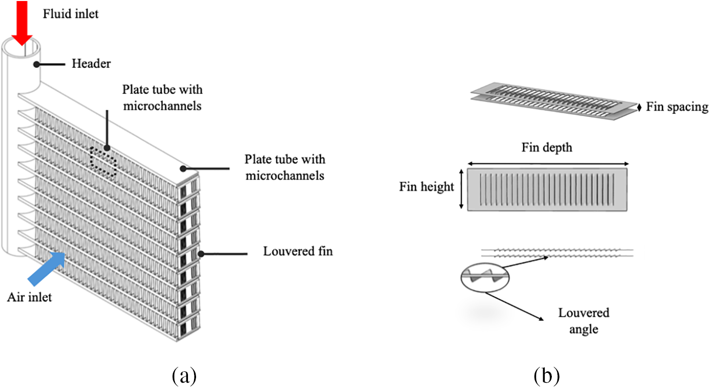
Figure 2: (a) The schematic microchannel heat exchangers, (b) The schematic fin of microchannel heat exchangers
2.2 CFD Model and Mesh Sensitivity Analysis
A minimal repeating unit containing a fin was taken as the computational domain. The air domain extends upstream by twice and downstream by three times to minimize the effects of the inlet and outlet boundary conditions. The mesh division and boundary settings are shown in Fig. 3. The air inlet and outlet are set as velocity inlet and pressure outlet, respectively. The two sides parallel to the fins are set as periodic boundaries, the central plane of the flat tube as a symmetry boundary, and the inner surface of the flat tube as a temperature boundary with a condensation temperature. Heat conduction through the fin into the flat tube is considered, ignoring contact thermal resistance. The inlet air velocity is set between 1 to 10 m/s, and the fin spacing is taken as the characteristic length. The Reynolds numbers under these operating conditions are less than 1200, hence a laminar flow model is used.
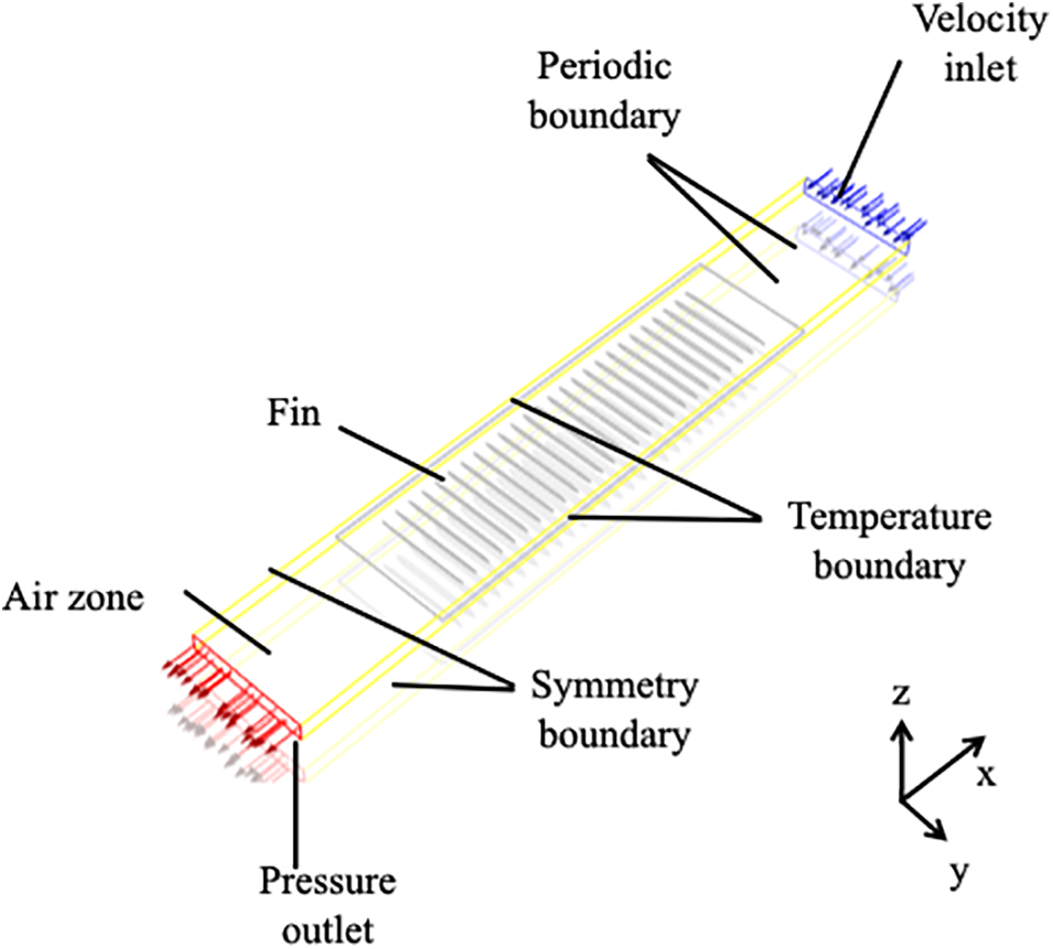
Figure 3: The CFD settings of microchannel heat exchanger fin simulation
The governing equations include the continuity equation, momentum equation, energy equation, and solid heat conduction equation. In ANSYS FLUENT version 2022R2, the flow and heat transfer module is used, employing the Coupled algorithm. The governing equations are discretized using the control volume method, and the convection terms are discretized using the power-law scheme. The error tolerance for the continuity and momentum equations is set at 10−6, and for the energy equation, it is set at 10−9.
For impressionable fluids, Conservation of Mass (Continuity Equation):
This implies that the velocity field of an incompressible flow must be divergence-free, a condition commonly referred to as the divergence-free constraint. It’s important to note that the continuity equation lacks a time derivative, even in the case of unsteady flows, which is one of the factors contributing to the complexity of numerically solving incompressible flows.
Conservation of Momentum:
where
where
In the above equation,
Fig. 4 illustrates the mesh independence verification performed in this study. The analysis shows that the deviation in pressure drop between a mesh resolution of 7 million and 20 million cells is less than 0.1%. Therefore, a mesh size of 7 million cells was chosen for the simulations, as it offers an optimal balance between accuracy and computational efficiency. This approach ensures reliable results while significantly reducing computational resource demands.
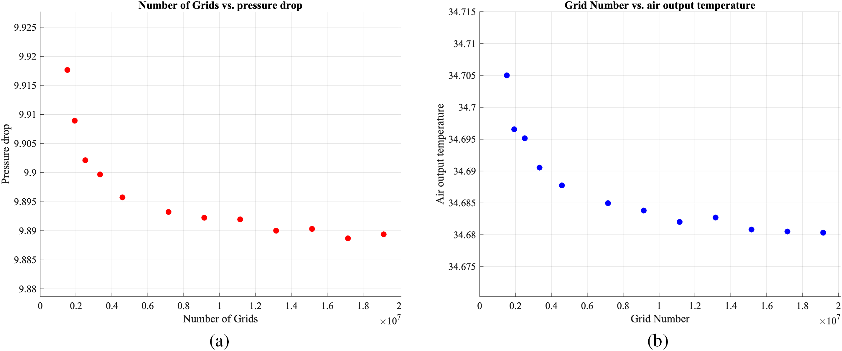
Figure 4: (a) The grid number sensitivity analysis of pressure drop; (b) The grid number sensitivity analysis of air outlet temperature
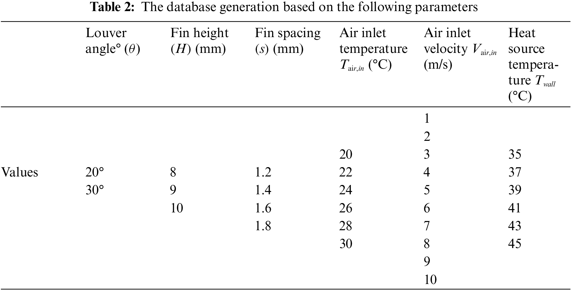
To develop any machine learning model, establishing a comprehensive database is necessary, As illustrate in Table 2, which shows the variables and values such as fin height, fin spacing, air inlet temperature, air inlet velocity, heat source temperature, the parameter ranges for louver angle, fin height, fin spacing, air inlet temperature, air inlet velocity, and heat source temperature were chosen based on common industry practices and achievable operational conditions in heat exchanger systems. These ranges ensure that the results are applicable to real-world scenarios and can be validated in future experimental setups. Using a full factorial design [22] ensures the completeness of the experimental database, resulting in a total of 9640 data points (2 * 3 * 4 * 6 * 11 * 6). Full factorial design is an experimental design method used to systematically investigate and evaluate the impact of multiple factors on one or more response variables [22]. In full factorial design, each level of every factor is combined with every level of all other factors, thus forming all possible combinations.
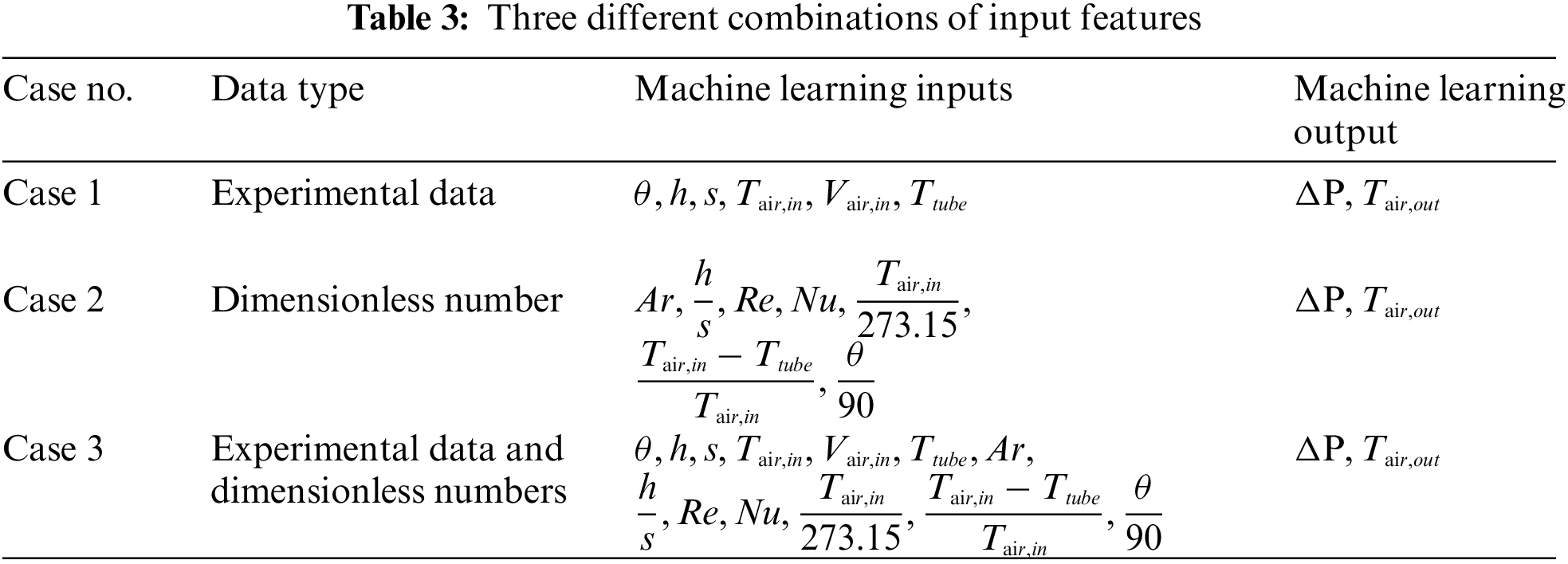
The selection of input features was strategically designed to optimize the predictive accuracy of the model, enhance its scalability, and eliminate any redundant variables. To systematically assess the influence of the impact of different input features on the model’s predictive performance, three distinct configurations of input features were explored as illustrated in Table 3. In this study,
2.4 Machine Learning Techniques
2.4.1 Artificial Neural Networks
ANNs are a category of machine learning techniques modeled after the structural and functional properties of the human brain. These networks consist of multiple processing units known as neurons [23,24]. Among the different types of ANNs, the feedforward neural network is the most widely used, particularly in engineering applications. A typical neural network includes an input layer, one or more hidden layers, and an output layer. Fig. 5 illustrates the architecture of a standard feedforward neural network.
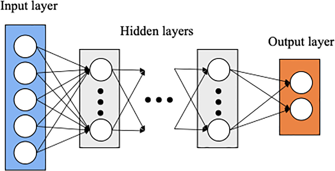
Figure 5: Schematic views of the ANN model
In the training phase, an ANN increases its prediction accuracy by refining the weights and biases of its neurons through a process referred to as “learning”. This iterative adjustment uses the backpropagation algorithm, a standard method for updating weights and biases in the field. Initially, weights are randomly set and then fine-tuned iteratively to reduce the variance between the actual outputs and the predicted ones. Neurons within each layer are linked to the subsequent layer via weights, and each neuron incorporates a bias, enhancing the network’s operational flexibility [25]. The operation of an ANN involves multiplying input features by their respective weights, adding these products to the biases of the neurons, and then summing these values to compute activation value [26]. Eq. (6) represents this process as a linear combination of the input features and their associated weights, complemented by a bias term. This combination forms the input to an activation function, introducing non-linearity which allows the neural network to effectively model the intricate relationships between inputs and outputs. The network adjusts these weights and biases to minimize prediction error [27].
where
2.4.2 Support Vector Machine (SVM)
During the training process, an SVM enhances its performance by optimizing the position of the decision boundary, aiming to maximize the margin between different class labels as indicated in Fig. 6. This optimization is achieved through an iterative approach that adjusts the parameters controlling the hyperplane [28]. Initially, parameters are selected based on specific criteria, and then refined to minimize errors such as misclassifications. In SVM, each data point contributes to the formation of the decision boundary based on its relative position to the margin. The computation involves dot products between input vectors and the vectors that define the hyperplane, adjusted by a bias term. This configuration ensures that the SVM can effectively separate classes with a hyperplane that maximizes the distance from the nearest points of all classes, known as support vectors. This strategic placement of the hyperplane allows the SVM to provide a robust model that is sensitive to the nuances of the input data distribution, thereby ensuring accurate classification or regression outputs [29].
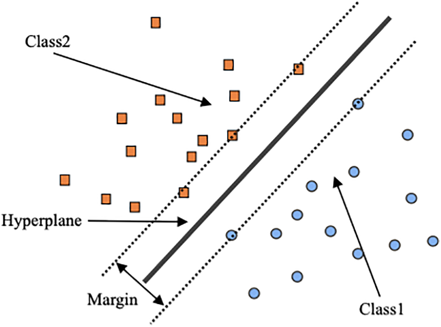
Figure 6: Schematic views of the SVM model
RF is a powerful machine learning algorithm primarily used for regression tasks which employs “bagging” to improve its robustness [25]. It operates by constructing multiple decision trees during the training phase, each trained on different subsets of data, as shown in Fig. 7. By randomly choosing features for each tree to split the data, RF ensures diversity among the trees, which helps reduce overfitting and enhance the model’s accuracy. During the prediction phase, RF consolidates the output by averaging the predictions from all trees, making the model effective in handling complex and high-dimensional datasets.
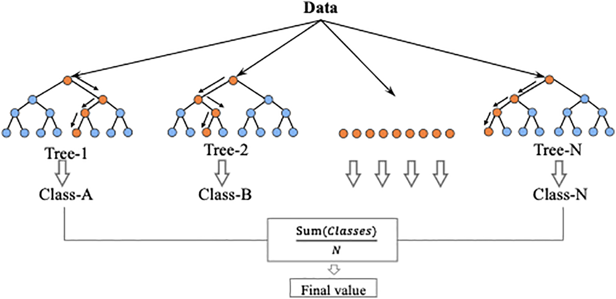
Figure 7: Schematic views of the RF model
As shown in Eq. (7), the mathematical formulation for RF in regression which averages the outputs
In this study, the Random Forest algorithm is employed for regression tasks to accurately predict key performance parameters of microchannel heat exchangers, specifically pressure drop and outlet air temperature. It is important to clarify that, in the context of regression, the outputs are inherently continuous rather than discrete. Consequently, the term “classes” used herein does not align with the conventional understanding as applied in classification tasks, where outputs are categorized into discrete classes. Instead, within this regression framework, “classes” refer to defined ranges or bands of continuous output values. Each decision tree within the Random Forest ensemble generates a continuous prediction for these parameters, and the collective output is computed as the mean of these individual predictions. This methodology diverges from classification approaches, where decision trees vote for discrete categories, and the category receiving the majority vote becomes the model’s output. Therefore, in the context of this research, “classes” are conceptualized as distinct performance intervals delineated by the continuous nature of the output values, providing a refined analytical framework for assessing heat exchanger performance.
2.4.4 Gaussian Process Regression (GPR)
GPR is an advanced Bayesian machine learning method that uses the multivariate Gaussian distribution assumption for regression analysis, independent of specific functional forms. Instead, it models relationships between data points through covariance functions such as the Radial Basis Function (RBF), Matérn kernel, and periodic kernels [30]. These kernels define the correlation between points in the input space and determine the smoothness and flexibility of the model. The training process of GPR involves maximizing the log-likelihood function to learn the data’s covariance structure. During the prediction phase, GPR uses the known data points and kernel functions to predict the output values and their uncertainties for new points, represented by the mean and standard deviation of the predictions. This prediction process not only provides the expected output for the predicted points but also accompanies it with measures of uncertainty, typically represented by the standard deviation [31]. The following diagram Fig. 8 illustrates training points are shown in red, while the predicted values and their uncertainties for other points are depicted with blue lines and light blue areas.
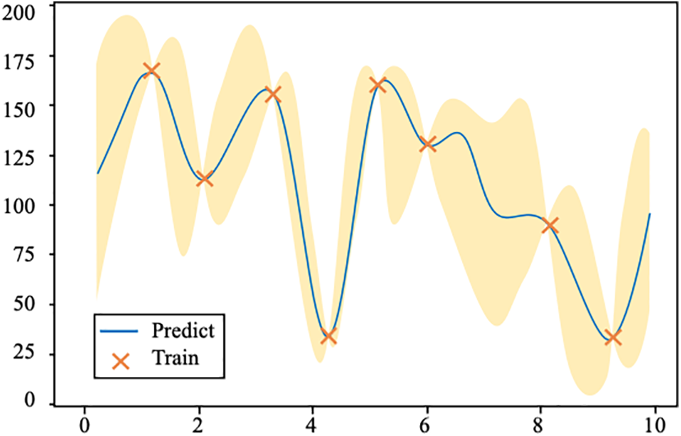
Figure 8: Schematic views of the GPR model
For the selection of dimensionless data, This research chose
By setting the tube wall as the heat source temperature, the tube wall temperature, airside inlet velocity, and airside inlet temperature are established. Finally, through the CFD model calculations, the airside outlet temperature and pressure drop can be obtained. The CFD model regresses the airside heat transfer coefficient. There are only tube wall thermal resistance and airside thermal resistance in the CFD model. The total heat transfer rate on the airside in the CFD model is calculated as follows:
The total heat transfer on the airside in the CFD model is calculated as follows:
Thermal resistance of the tube wall:
The calculation of the airside thermal resistance is as follows:
where m is an intermediate variable, and h is the height difference factor or geometric factor.
The airside heat transfer coefficient can be regressed by minimizing the residual, which is expressed as the square root of the sum of the squared differences between the calculated heat transfer
For the calculation of Reynolds number and Nusselt number:
3.2 Machine Learning Models and Results
This chapter introduces the setup of four models, including their respective prediction accuracies. For the error calculation of the four models, various statistical metrics are presented, including Root Mean Square Error (RMSE), Mean Squared Error (MSE), Mean Absolute Error (MAE), and the coefficient of determination (R2). These metrics provide a detailed reflection of the models’ performance on testing datasets from different perspectives as illustrated in Table 3. RMSE is sensitive to large errors and penalizes significant deviations, making it ideal for detecting substantial prediction discrepancies. MSE, being similar to RMSE but without the square root, provides an average error measure and is commonly used for model optimization as it emphasizes larger errors. MAE, on the other hand, treats all errors equally by taking the absolute difference, offering a straightforward interpretation of the average error without overemphasizing outliers. Finally, R2 indicates how well the model’s predictions match the actual data, with values closer to 1 showing that the model effectively explains the variability in the data. These indicators were selected to provide a comprehensive evaluation of the model’s performance, covering multiple perspectives such as error sensitivity and overall model fit.
The mathematical equations for each type of error metric used are presented below. The RMSE is another widely utilized regression metric. It is computed by first squaring the differences between each observed value and its corresponding predicted value, then averaging these squared differences, and finally taking the square root. The formula for RMSE is:
MSE is a metric used to evaluate the accuracy of an estimator—it is always non-negative, with lower values indicating better performance, and values closer to zero being ideal. Unlike the RMSE, MSE does not take the square root. MSE is calculated by taking the squares of the differences between predicted and observed values, summing them up, and dividing by the number of observations. The formula for MSE is:
MAE is another metric used to evaluate the accuracy of an estimator. It is always non-negative, with values closer to zero indicating higher accuracy. Unlike RMSE, MAE does not square the errors. Instead, it is calculated by taking the absolute differences between the predicted and observed values, summing these differences, and then dividing by the number of observations. The formula for MAE is:
R2 also referred to as the coefficient of determination, is used to assess how effectively the model accounts for the variability in the observed values. It ranges from 0 to 1, with values closer to 1 signifying a better fit. The formula is:
The dataset was randomly partitioned into a training set and a test set, with 80% of the data used to train the model, and the remaining 20% used to assess the model’s predictive performance. To address potential issues with input feature scaling, data normalization is conducted, standardizing all input features to the range [0, 1]. This step is crucial as it helps optimize the training process by preventing gradient issues that can arise from large differences in feature scales.
The constructed neural network is based on a feedforward architecture, where the core of the network is a hidden layer containing 10 neurons. The size of this hidden layer was determined based on the complexity of the problem, and this study tested grid structures with 5, 10, 20, and 30 neurons. The following formula represents the time complexity calculation model for the neural network structure:
In this formula,
The results show that using 10 layers yields higher predictive accuracy compared to 5 layers, while significantly reducing computational load compared to using 20 or 30 layers. Additionally, this study tested network structures with 1, 2, and 3 hidden layers, and the results indicated that computation time increases exponentially with 2 and 3 layers. Considering both computational cost and accuracy, a network structure with 1 hidden layer and 10 neurons was selected.
According to Wilson’s research [32], in gradient descent algorithms like error backpropagation, the learning rate significantly impacts generalization accuracy. Lowering the learning rate below the level for fastest convergence can improve accuracy, especially for complex problems. A learning rate of 0.01 is considered an appropriate choice, as it strikes a balance that avoids overfitting while maintaining prediction accuracy during training. The training configuration of the neural network includes 2000 training iterations, and an error target of 10−9 which are configured to prevent the model from training indefinitely, providing a clear stopping criterion. During training, the network automatically adjusts the weights and biases to minimize prediction error. In this process, 80% of the data is used for training, with 15% of that data reserved for validation to prevent overfitting. After completing the predictions, denormalization is performed, converting the predicted results back to their original scale, making it easier to compare them with the actual values.
As shown in Figs. 9–11, which present the prediction accuracy of the ANN model based on the Case 1, Case 2, Case 3 database, separately: Part (a) illustrates the accuracy of pressure drop predictions, while Part (b) details the accuracy for air outlet temperature predictions, both derived from the testing set of the database. In both subfigures, the x-axis represents the actual values, and the y-axis represents the predicted values. In Case 3, which shows the highest prediction accuracy. The close alignment of the data points along the ideal prediction line indicates that the model performs exceptionally well, demonstrating its robustness and precision in forecasting complex phenomena within the specified parameters.

Figure 9: Case 1: (a) ANN prediction accuracy of heat exchangers pressure drop; (b) ANN prediction accuracy of heat exchangers air outlet temperature
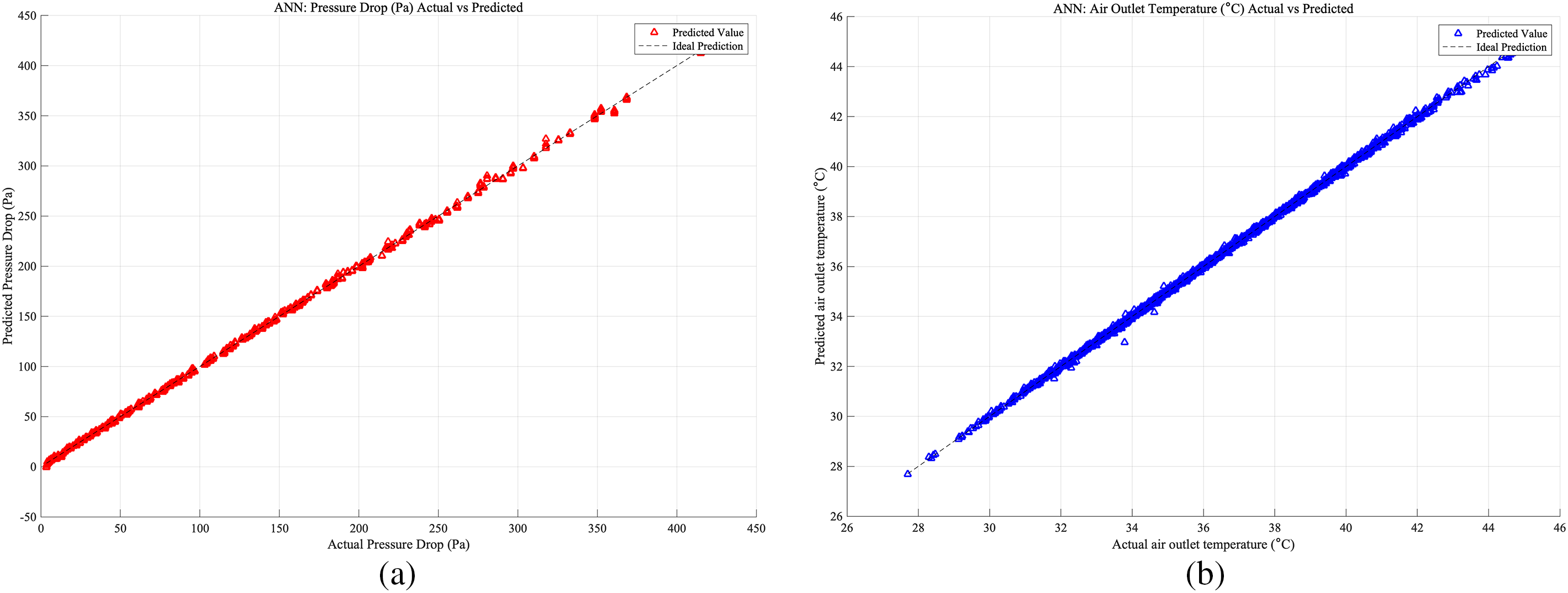
Figure 10: Case 2: (a) ANN prediction accuracy of heat exchangers pressure drop; (b) ANN prediction accuracy of heat exchangers air outlet temperature
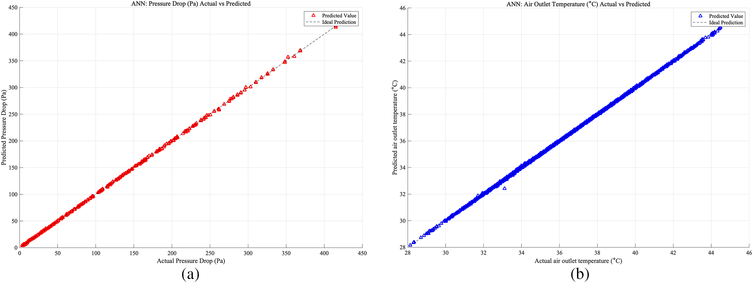
Figure 11: Case 3: (a) ANN prediction accuracy of heat exchangers pressure drop; (b) ANN prediction accuracy of heat exchangers air outlet temperature
For the SVM model setup, the database was divided in the same way as for the ANN model. As shown in Figs. 12–14, which present the prediction accuracy of the SVM model based on the Case 1, Case 2, and Case 3 databases, respectively, the prediction accuracy is highest for Case 3 under the SVM model.
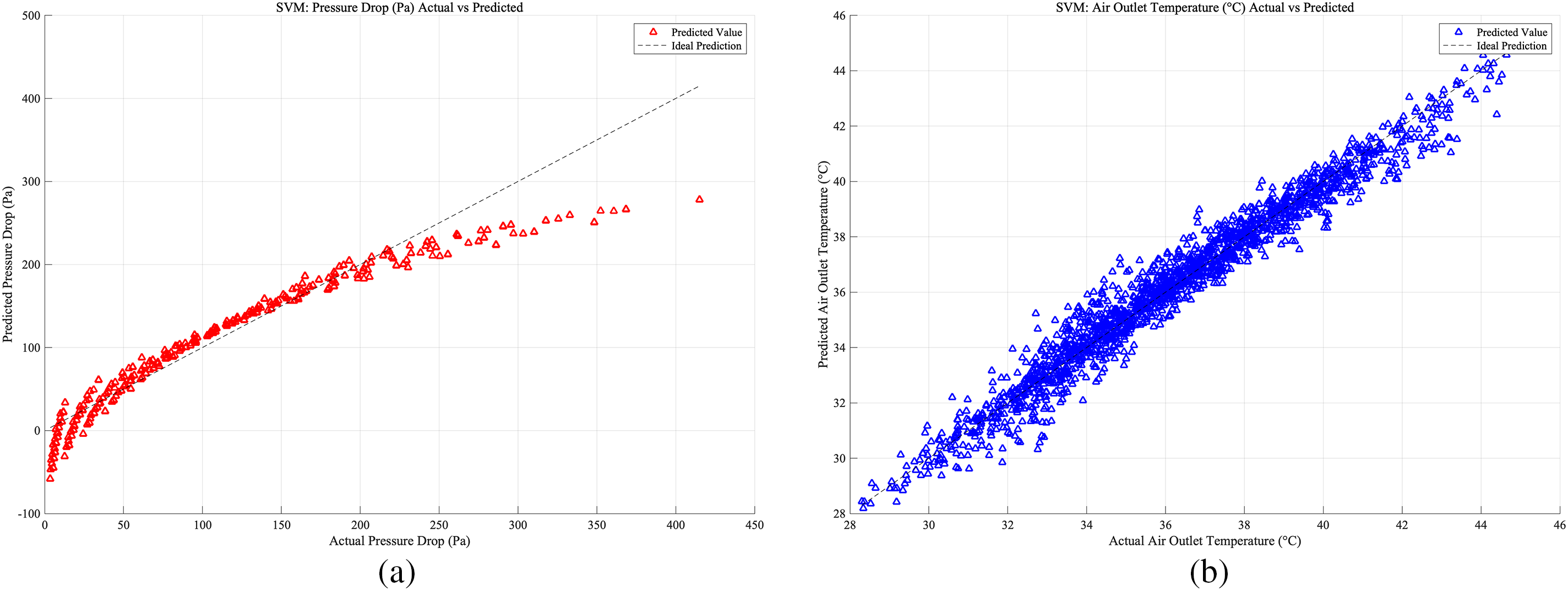
Figure 12: Case 1: (a) SVM prediction accuracy of heat exchangers pressure drop; (b) SVM prediction accuracy of heat exchangers air outlet temperature
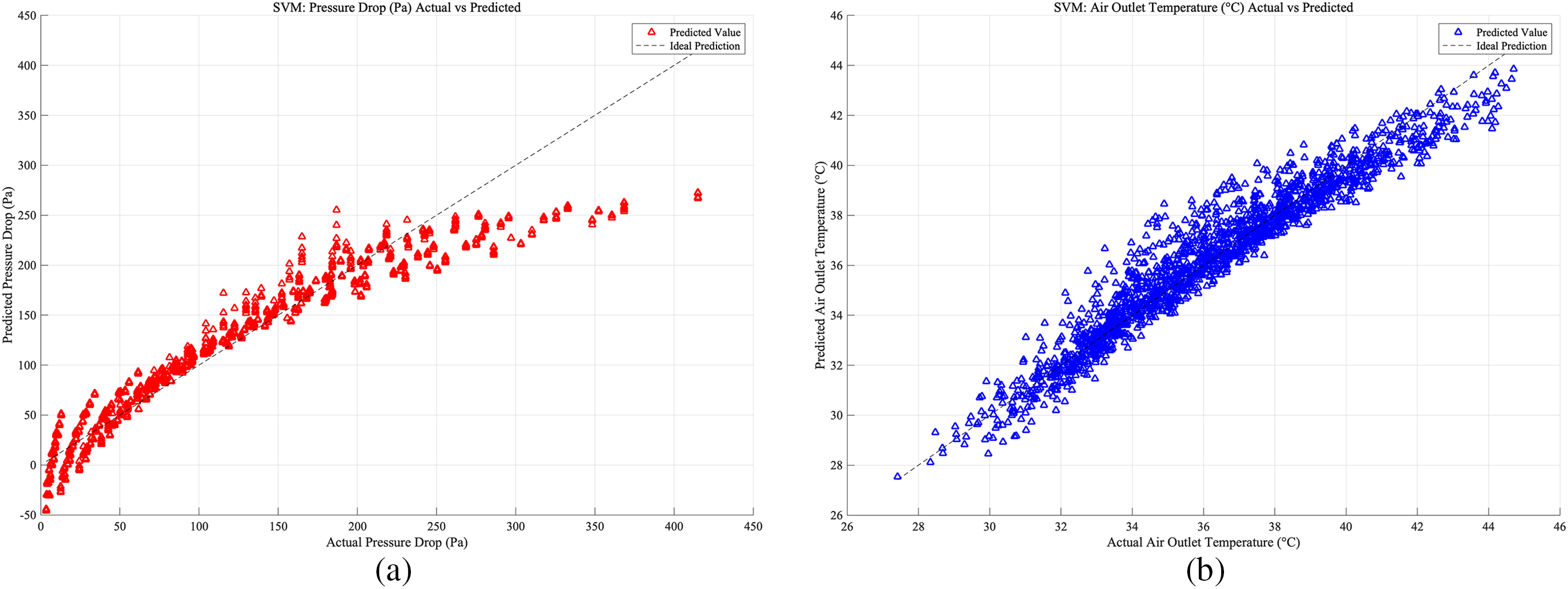
Figure 13: Case 2: (a) SVM prediction accuracy of heat exchangers pressure drop; (b) SVM prediction accuracy of heat exchangers air outlet temperature
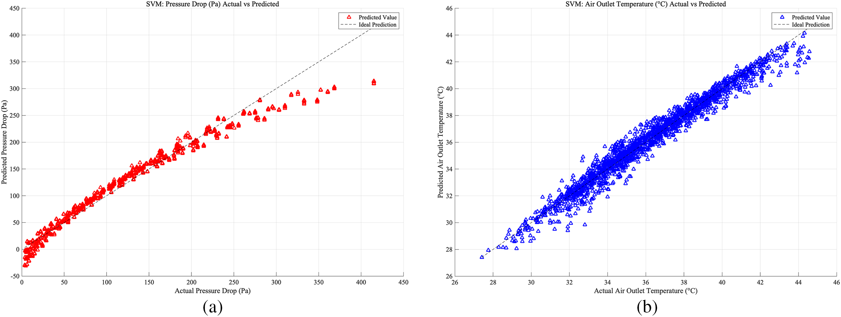
Figure 14: Case 3: (a) SVM prediction accuracy of heat exchangers pressure drop; (b) SVM prediction accuracy of heat exchangers air outlet temperature
In the RF model, two separate random forest models were created, with each model predicting a different output variable. According to Breiman’s research [33], each leaf, or terminal node, of individual trees typically contains a limited number of observations, generally ranging from 1 to 5. According to Probst et al. [34], for most of the examined datasets, the biggest performance gain is achieved when training the 100 trees. The model construction specified the number of trees (100 trees) and the minimum number of samples per leaf node 5, parameters that influence the model’s complexity and fitting accuracy.
As shown in Figs. 15–17, which present the prediction accuracy of the RF model based on the Case 1, Case 2, Case 3 database, separately. For the RF models across the three cases, the prediction accuracy was lowest for the Case 1 database, while the best prediction results were obtained for the Case 3 database.
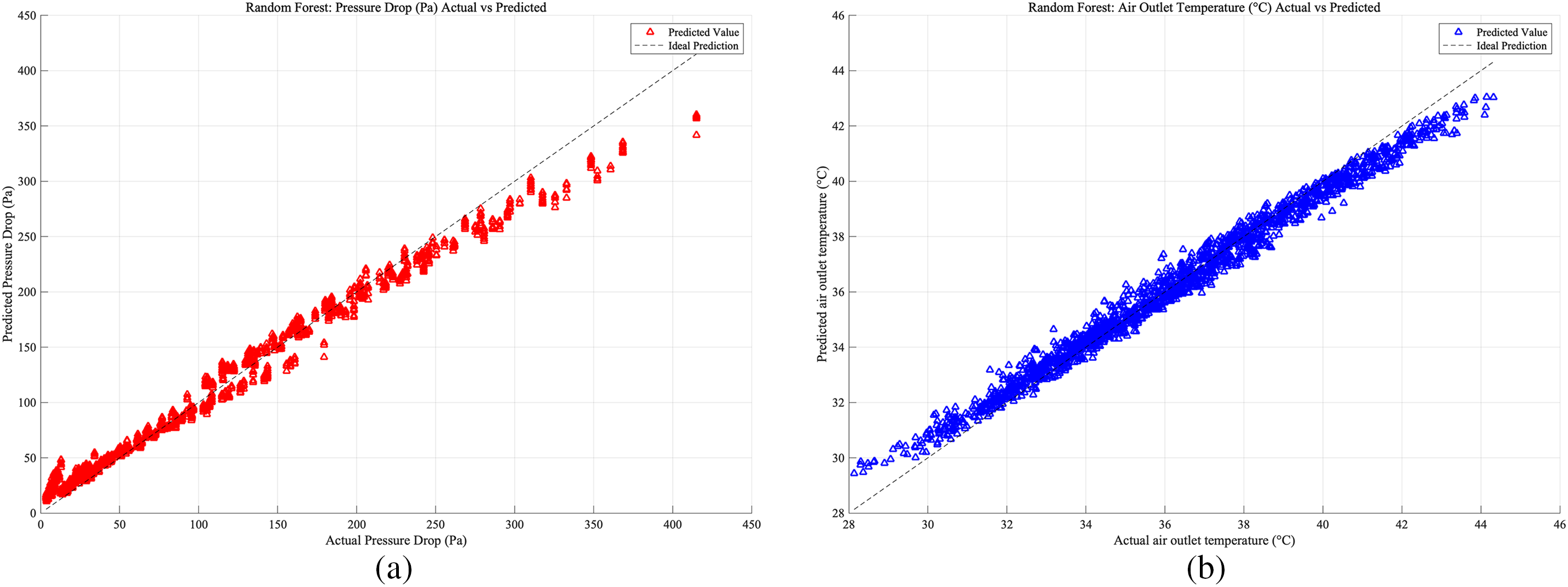
Figure 15: Case 1: (a) RF prediction accuracy of heat exchangers pressure drop; (b) RF prediction accuracy of heat exchangers air outlet temperature
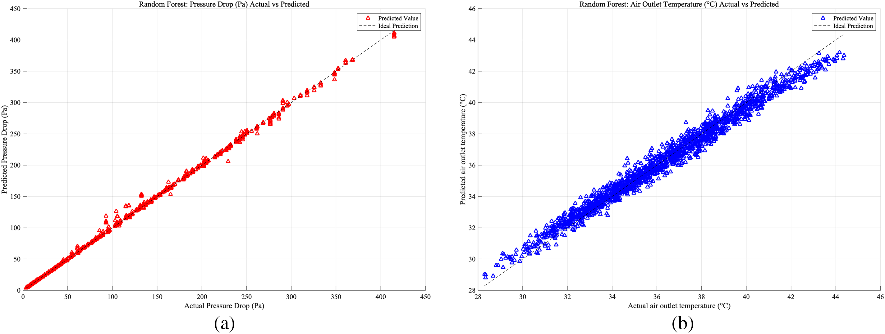
Figure 16: Case 2: (a) RF prediction accuracy of heat exchangers pressure drop; (b) RF prediction accuracy of heat exchangers air outlet temperature
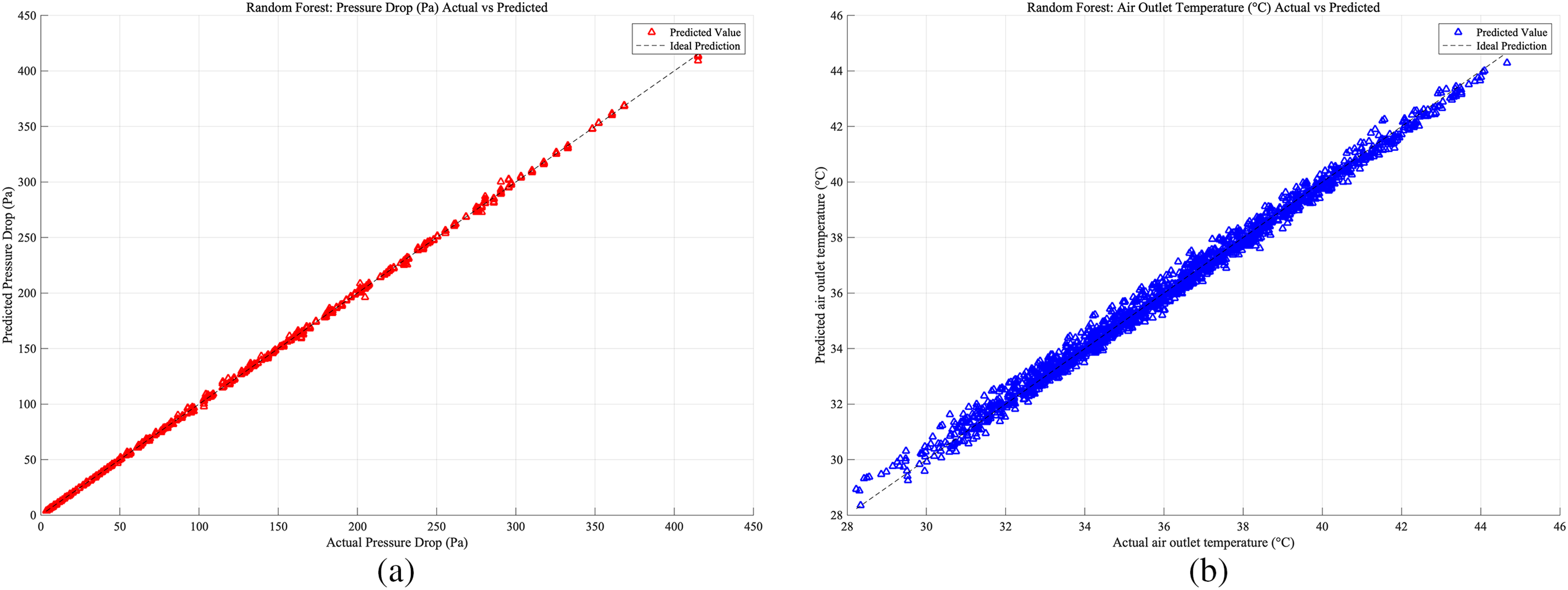
Figure 17: Case 3: (a) RF prediction accuracy of heat exchangers pressure drop; (b) RF prediction accuracy of heat exchangers air outlet temperature
For the GPR model, the fitrgp function was used, which is a function of MATLAB version R2023b for fitting Gaussian Process Regression models. Based on the provided input data and target output, it creates a GPR model for regression tasks. The squared exponential kernel function was used, which defines similarity based on the Euclidean distance between input points. The formula for this kernel function is as follows:
•
•
As shown in Figs. 18–20, which present the prediction accuracy of the GPR model based on the Case 1, Case 2, and Case 3 databases, respectively, the model predictions are highly accurate across all three cases.
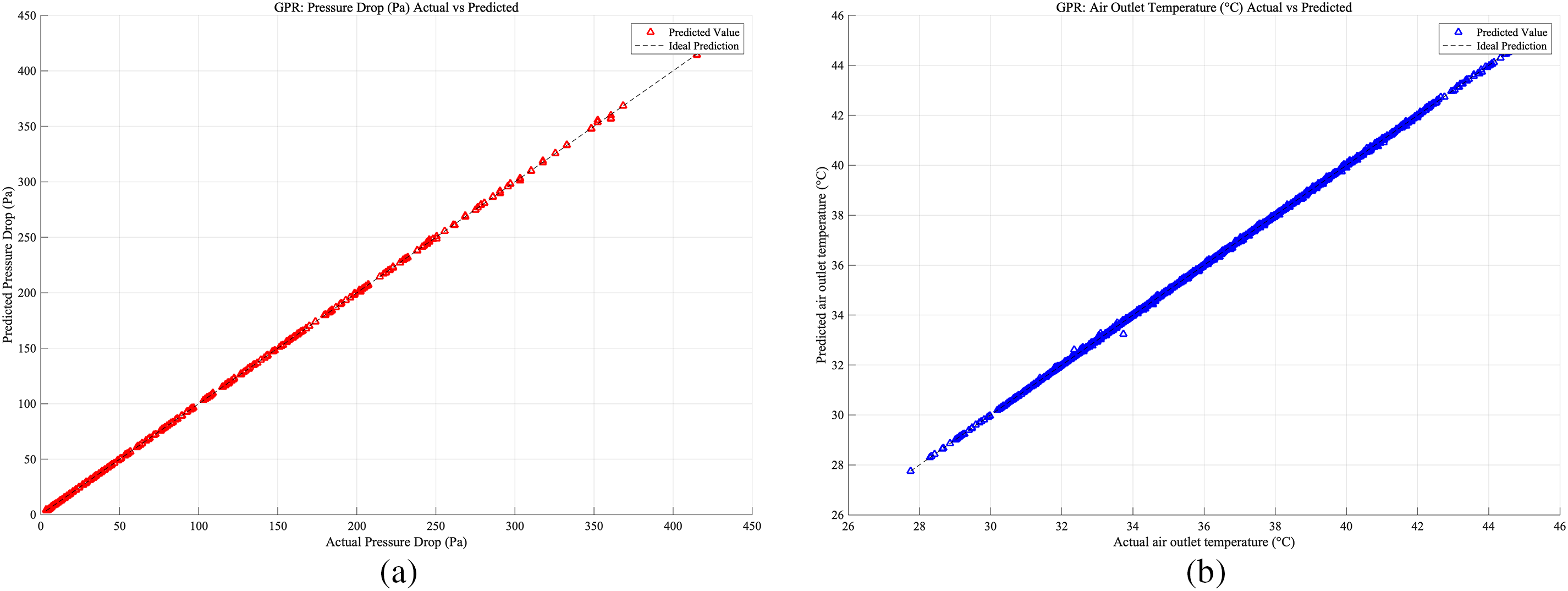
Figure 18: Case 1: (a) GPR prediction accuracy of heat exchangers pressure drop; (b) RF prediction accuracy of heat exchangers air outlet temperature
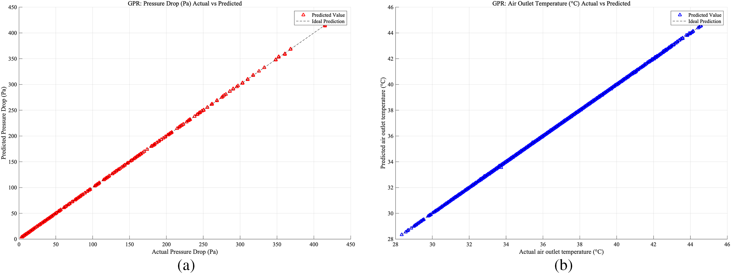
Figure 19: Case 2: (a) GPR prediction accuracy of heat exchangers pressure drop; (b) RF prediction accuracy of heat exchangers air outlet temperature
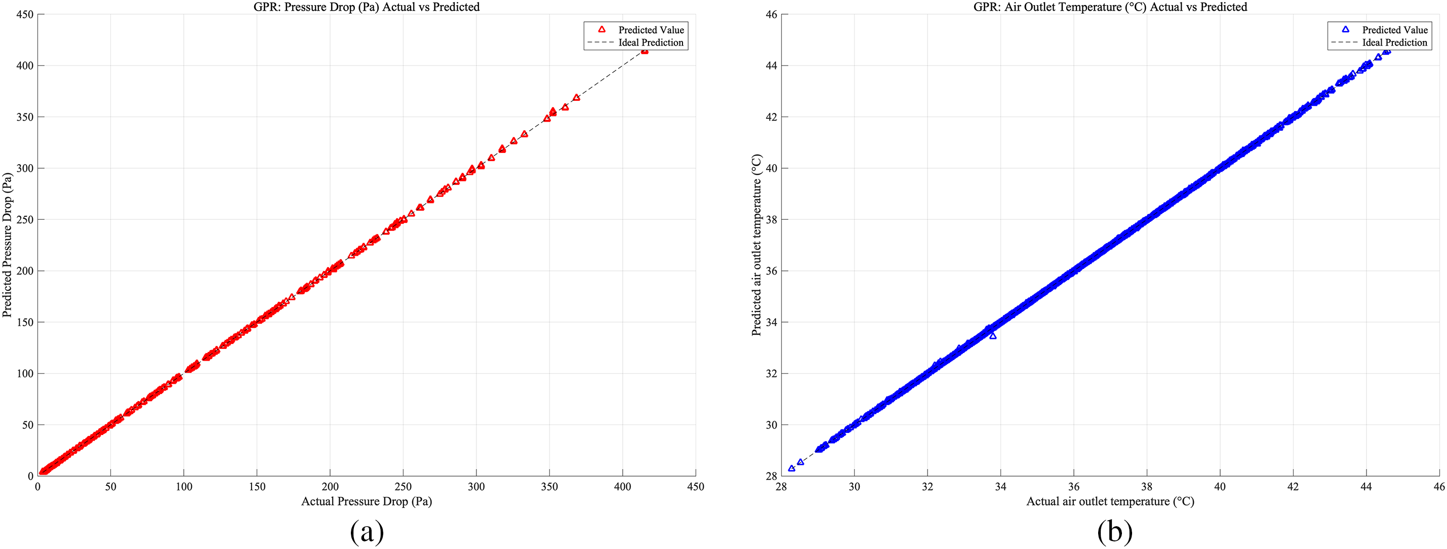
Figure 20: Case 3: (a) GPR prediction accuracy of heat exchangers pressure drop; (b) RF prediction accuracy of heat exchangers air outlet temperature
The following three heatmaps illustrate the correlations between various input parameters and output parameters. In each heatmap, the color gradient transitions from white to black, where black indicates strong positive correlations and white indicates strong negative correlations. Orange is used to represent a zero-correlation coefficient, signifying no correlation between the parameters.
As shown in Fig. 21, this chart presents the correlation between basic parameters in the Case 1 database, such as temperature
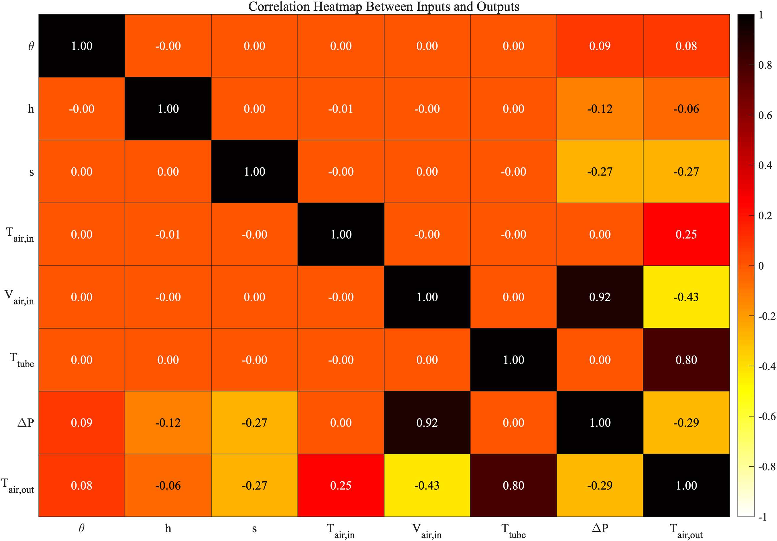
Figure 21: The database parameters heatmap of Case 1
As shown in Fig. 22, this figure introduces more dimensions, such as
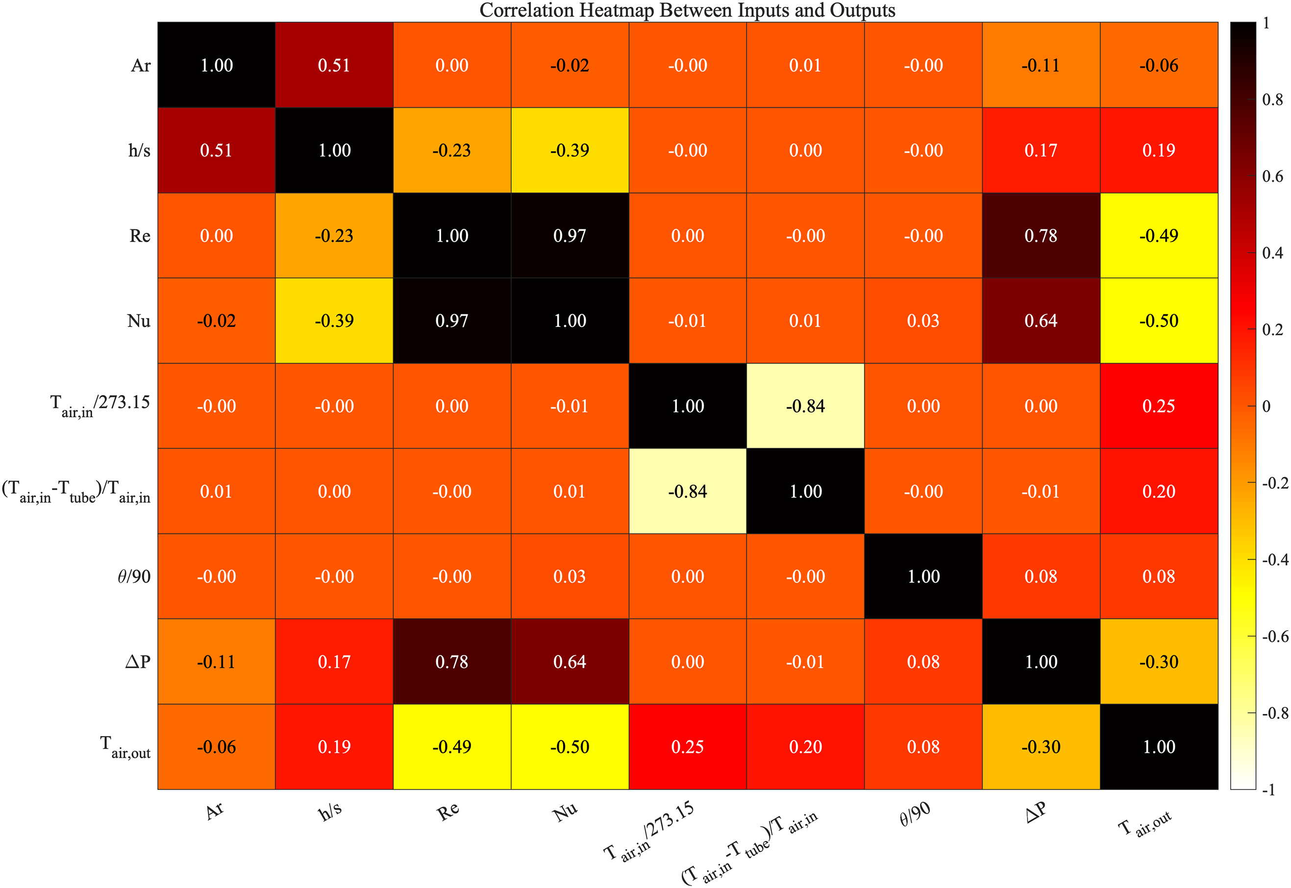
Figure 22: The database parameters heatmap of Case 2
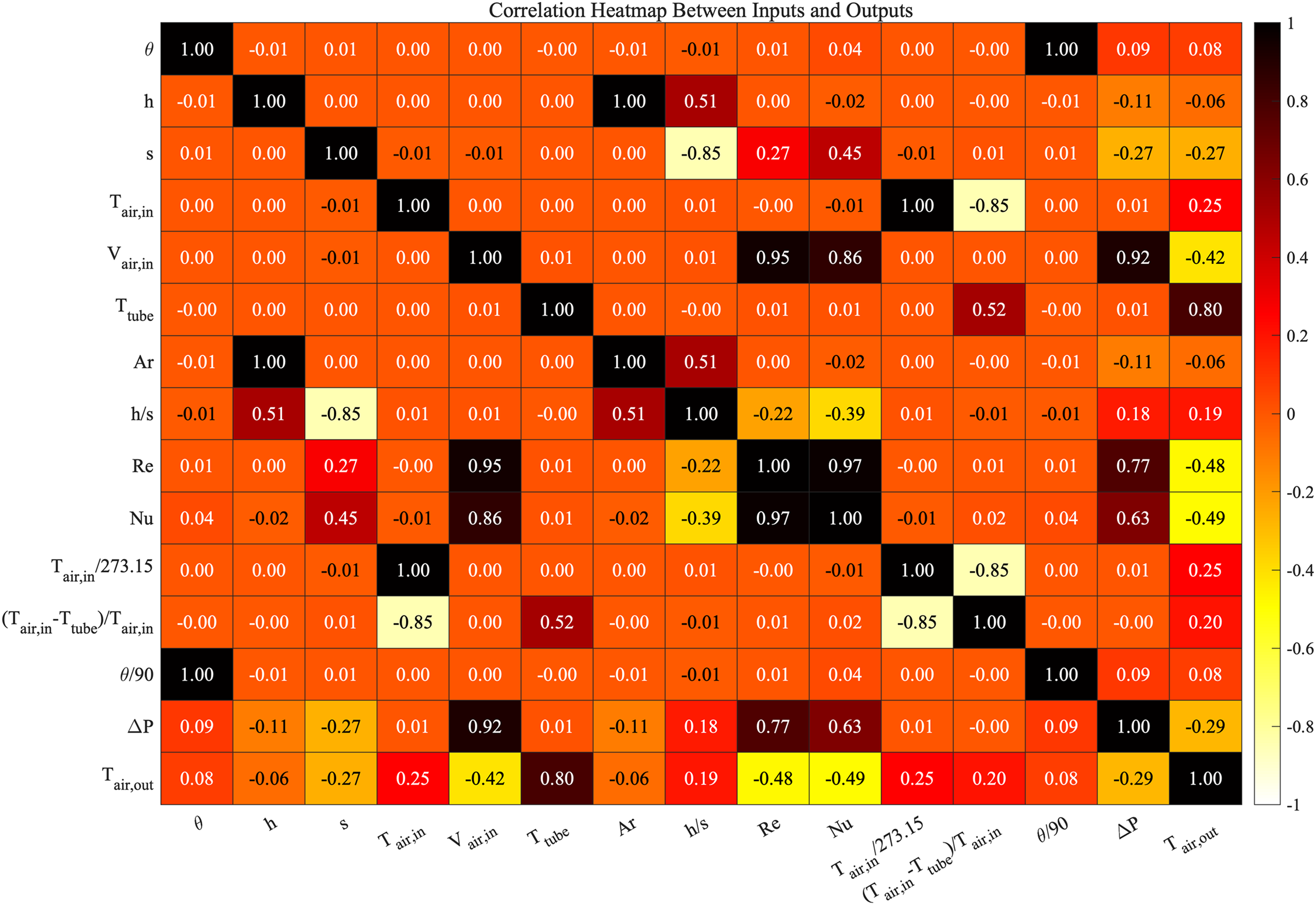
Figure 23: The database parameters heatmap of Case 3
The summarized results from the Table 4 illustrates the comparative performance of various machine learning models, ANN, SVM, RF and GPR which are applied to predict two critical parameters of microchannel heat exchangers: pressure drop and air outlet temperature. These metrics are evaluated across three distinct cases using standard error metrics including RMSE, MSE, MAE, and R2.
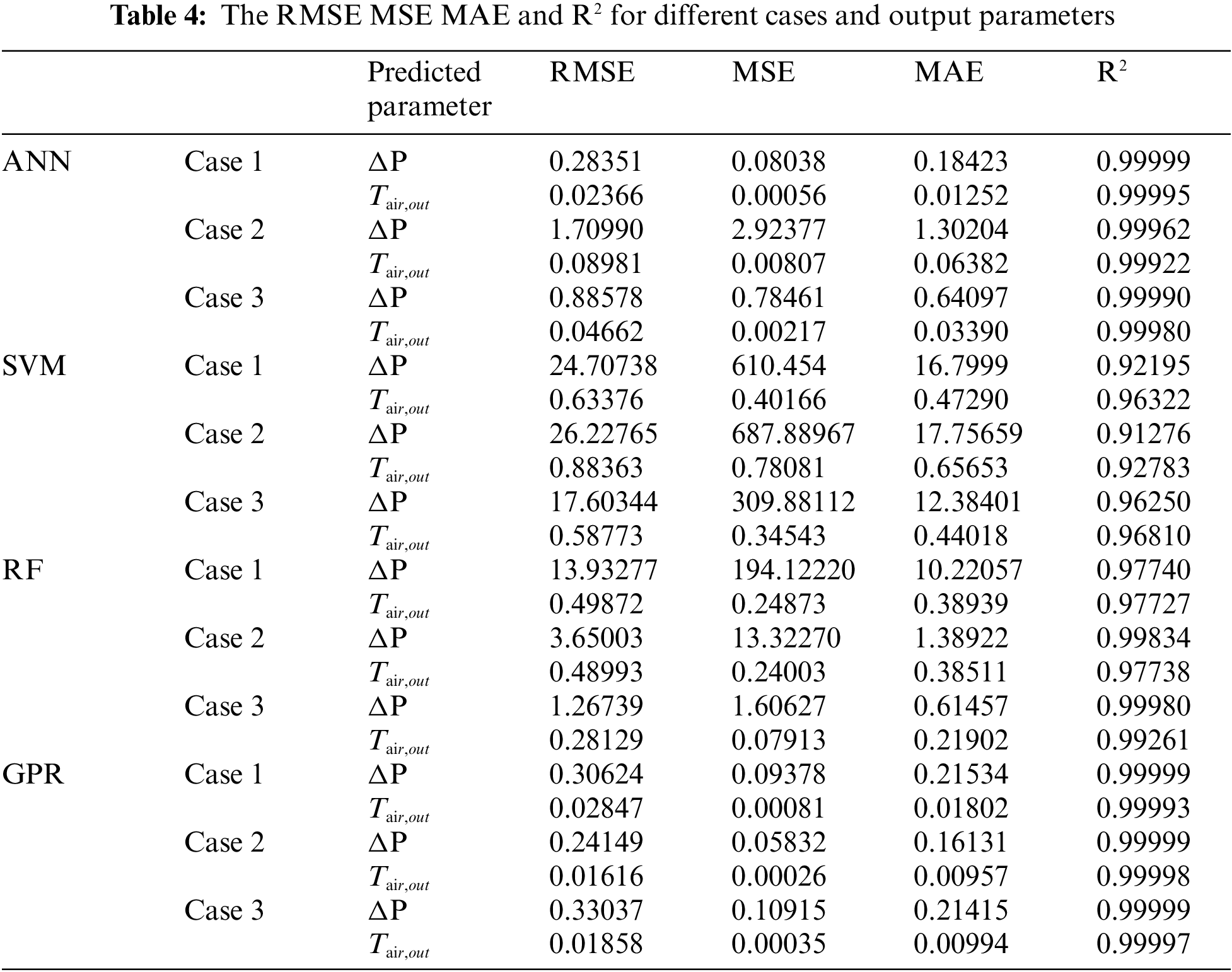
1. ANN demonstrated robust predictive capabilities, achieving nearly perfect R2 values close to 1.00 in all scenarios. This was particularly evident in the pressure drop predictions, where the ANN model maintained high accuracy and low error metrics, substantiating its suitability for complex physical phenomena modeling in heat exchanger systems.
2. SVM exhibited higher errors and lower R2 values, indicating a less favorable performance, particularly in handling the non-linear complexities associated with the data set for pressure drop predictions. These results suggest that without additional parameter tuning or kernel adjustments, SVM may not provide the most reliable predictions in this specific application.
3. RF performed commendably, especially in Case 3, where it achieved low RMSE values for pressure drop predictions. The consistently high R2 values for outlet temperature predictions across the cases indicate RF’s effectiveness in capturing the variability in the data, making it a dependable choice for scenarios where model interpretability and robustness against overfitting are priorities.
4. GPR showed exceptional accuracy, with RMSE and MSE values considerably lower than those of other models, coupled with R2 values nearing 1.00 for both pressure drop and outlet temperature in all cases. This performance underscores GPR’s capability in offering precise and reliable predictions, making it highly suitable for applications demanding high levels of predictive fidelity.
As shown in Fig. 24, based on the enhanced visual analysis provided by the comparative figures, it is clearer that the GPR model consistently outperforms other models in terms of predictive accuracy across all error metrics (RMSE, MAE, MSE, and R2). This is evident in the data for both pressure drop and air outlet temperature, where GPR exhibits the lowest error values. Following GPR, the next highest predictive accuracy is observed in the ANN model, followed by the RF model, while the SVM model demonstrates the lowest performance in comparison.
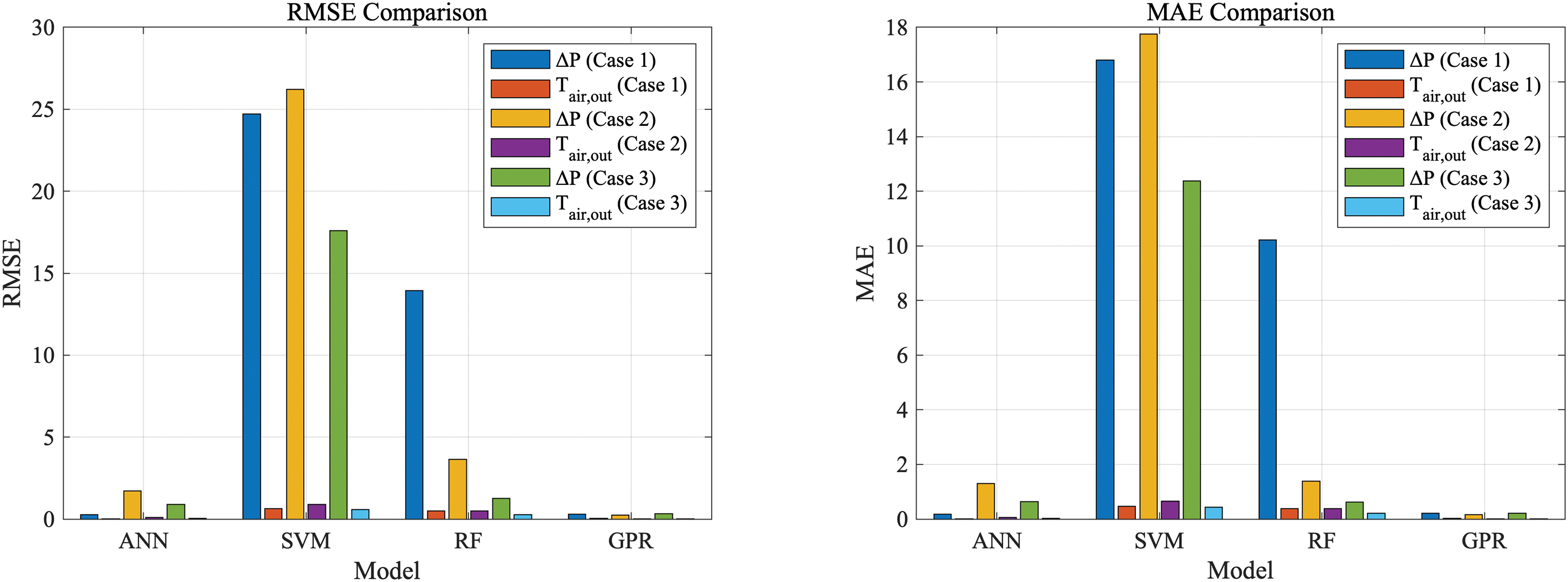
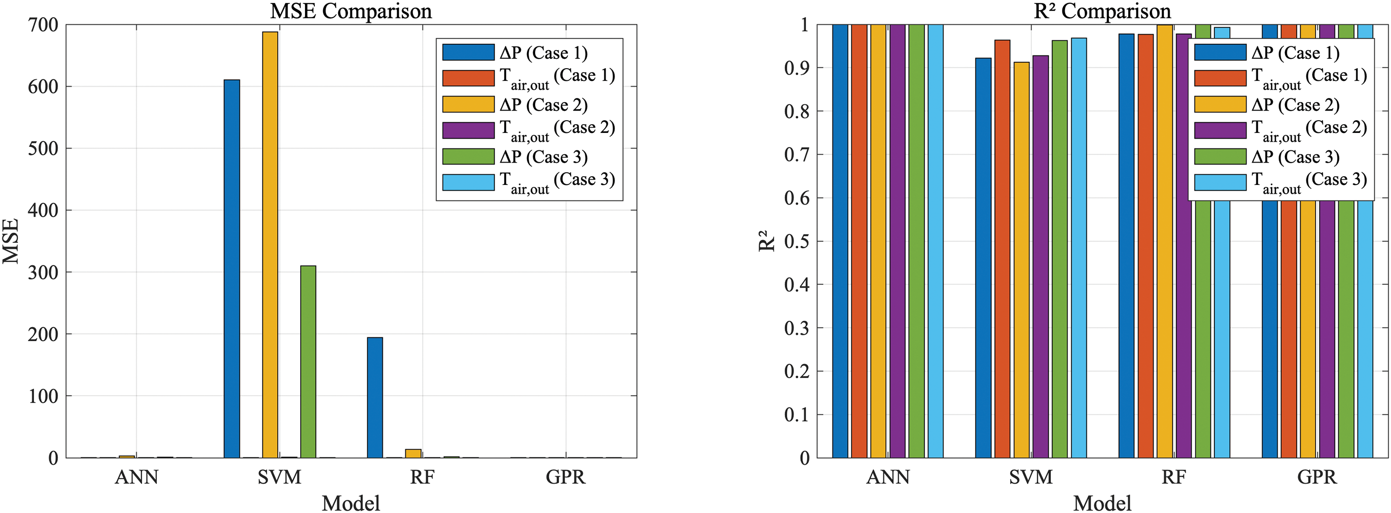
Figure 24: The RMSE MSE MAE and R2 for different cases and output parameters
Furthermore, when comparing performance across different datasets (Case 1, Case 2, and Case 3), the results indicate that Case 3 yields the best overall predictive accuracy in all models. This suggests that the underlying data in Case 3 is more conducive to producing accurate predictions, irrespective of the model applied. The charts clearly show that Case 3 achieves the lowest errors in all metrics, indicating its superior performance for training and model generalization.
Although GPR demonstrates high predictive accuracy, particularly in Case 1 and Case 3, ANN has a clear advantage in training time, being more computationally efficient than GPR when compare the training time for each model as shown in Fig. 25.
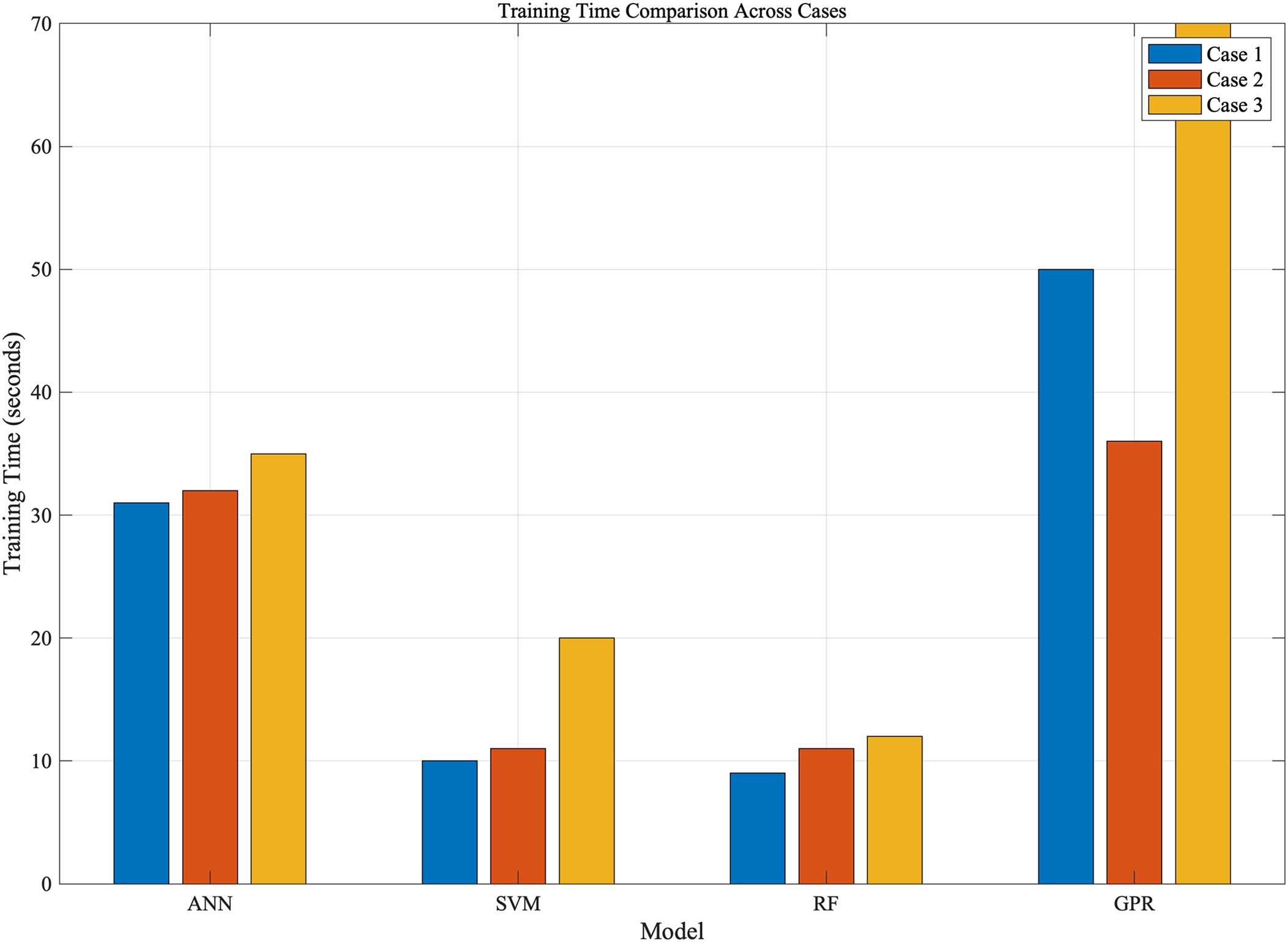
Figure 25: The training time for different cases and different machine learning model
To further the research in the field of microchannel heat exchangers using machine learning, several advanced directions are proposed:
1. Automated Dimensional Analysis: Future research should develop algorithms capable of automatically identifying and incorporating key dimensionless parameters, such as Reynolds and Nusselt numbers, into predictive models. This includes employing advanced feature selection and dimensionality reduction techniques to optimize the models’ performance across various operational settings.
2. Diverse Louver Configurations: Expanding the research to include a variety of louver configurations, such as different numbers and spacings of louvers, is crucial. Detailed investigations into how these variations affect thermal and fluid dynamics can yield valuable insights into optimizing heat exchanger designs for enhanced efficiency.
3. Comprehensive Data Collection: Enhancing the database with a wider array of experimental and simulated data covering various fin structures and operational conditions is essential. This expansion will help in refining the models to better generalize across different systems and conditions, thus improving their predictive robustness.
To enhance the performance of ANN models, employing Genetic Algorithms (GA) to improve the network architecture and hyperparameters. This approach allows for the systematic and automated selection of the best network settings, such as the number of hidden layers, neurons per layer, and learning rates, which are crucial for balancing model complexity and computational efficiency. By employing GA, ANN model can achieve higher predictive accuracy while managing computational resources effectively.
RF benefits significantly from tuning the number and depth of trees, which directly influences its robustness and ability to generalize. Increasing the number of trees can reduce variance without increasing bias, albeit at a higher computational cost. Fine-tuning the tree depth helps manage the model’s complexity, preventing overfitting while capturing sufficient data specifics. Additionally, implementing advanced feature selection methods can remove irrelevant inputs and improve model accuracy. Adjusting bootstrap sampling methods, such as using stratified or cluster sampling, can also optimize performance, especially in diverse datasets.
SVM is particularly sensitive to the choice of kernel and the scale of features. Selecting the appropriate kernel such as, linear, polynomial, and optimizing its parameters are critical for capturing the underlying patterns of the data. Regularization parameter tuning is crucial for balancing margin maximization and classification error minimization. Properly scaling and normalizing features can dramatically improve SVM’s performance, making it essential for preprocessing steps. Additionally, adjusting class weights can help the SVM model perform better on imbalanced datasets.
GPR while providing high accuracy and flexibility in handling complex datasets, struggles with computational demands when scaling to large datasets. Implementing sparse GPR models using techniques such as inducing points can significantly reduce the computation and memory requirements by approximating the full covariance matrix. Selecting simpler kernel functions or those that exploit data structure can also lessen computational burdens. Moreover, utilizing parallel computing frameworks to handle large-scale matrix operations can expedite both training and prediction phases, making GPR feasible for larger datasets.
This study highlights the significant potential of machine learning models in predicting the performance of microchannel heat exchangers, particularly focusing on critical operational parameters such as pressure drop and air outlet temperature. By conducting a detailed comparative analysis of four advanced algorithms: ANN, SVM, RF, and GPR. The main findings can be summarized as follows:
1. The foundational element of this research is the creation of an extensive database built from CFD simulations. This database encompasses a detailed range of operational parameters, providing a robust foundation for applying machine learning algorithms.
2. A comparative analysis among four advanced machine learning models—ANN, SVM, RF, and GPR—highlights their individual and collective capabilities. The results indicate that ANN and GPR exhibit superior precision, achieving remarkably high R2 values, demonstrating their effectiveness in modeling complex thermal interactions.
3. The use of dimensionless numbers improves prediction accuracy. By incorporating parameters such as Reynolds number, Nusselt number, and aspect ratio, the models can achieve a deeper insight into the heat transfer mechanisms, thereby enhancing their predictive accuracy and reliability.
Overall, this research explores the critical need for selecting suitable machine learning techniques when constructing databases that incorporate dimensionless numbers for modeling microchannel heat exchangers. It showcases the precise accuracy attainable by leveraging CFD simulations to assess heat transfer performance. The innovative integration of machine learning with CFD data provides essential insights for the rapid and iterative optimization of heat exchanger designs. These findings not only contribute valuable perspectives for swiftly and accurately evaluating heat exchanger performance but also facilitates a more streamlined design process and leads to advancements in the efficiency and effectiveness of heat exchanger modeling.
Acknowledgement: The authors are grateful for the support of Institute of Wenzhou, Zhejiang University.
Funding Statement: This research was supported by the National Natural Science Foundation of China (Grant No. 52306026), the Wenzhou Municipal Science and Technology Research Program (Grant No. G20220012), the Special Innovation Project Fund of the Institute of Wenzhou, Zhejiang University (XMGL-KJZX202205), and the State Key Laboratory of Air-Conditioning Equipment and System Energy Conservation Open Project (Project No. ACSKL2021KT01). The APC was also covered by the Special Innovation Project Fund of the Institute of Wenzhou, Zhejiang University (XMGL-KJZX-202205).
Author Contributions: Study conception and design: Long Huang, Baoqing Liu, Jinyuan Qian and Zhijiang Jin; data collection: Long Huang and Junjia Zou; analysis and interpretation of results: Long Huang and Junjia Zou; draft manuscript preparation: Long Huang and Junjia Zou; supervision: Baoqing Liu and Zhijiang Jin; project administration: Long Huang; funding acquisition: Long Huang and Jinyuan Qian. All authors reviewed the results and approved the final version of the manuscript.
Availability of Data and Materials: The data presented in this study are available on request from the corresponding author.
Ethics Approval: Not applicable.
Conflicts of Interest: The authors declare no conflicts of interest to report regarding the present study.
References
1. Olatunji KO, Madyira D. Enhancing the biomethane yield of groundnut shells using deep eutectic solvents for sustainable energy production. Front Energy Res. 2024 Feb 19;12. doi:10.3389/fenrg.2024.1346764. [Google Scholar] [CrossRef]
2. Singh A, Sahu D, Prakash Verma O. Study on performance of working model of heat exchangers. Mater Today: Proc. 2022 Sep;80:8–13. doi:10.1016/j.matpr.2022.09.373. [Google Scholar] [CrossRef]
3. Hall S. 2-Heat exchangers. In: Hall S, editor. Branan’s rules of thumb for chemical engineers. 5 ed. Oxford: Butterworth-Heinemann; 2012. p. 27–57. Available from: https://www.sciencedirect.com/science/article/pii/B9780123877857000025. [Accessed 2024]. [Google Scholar]
4. Ren T, Hrnjak P. Pressure drop in round cylindrical headers of parallel flow MCHXs: pressure loss coefficients for single phase flow. Int J Refrig. 2015;49:119–34. [Google Scholar]
5. Prithiviraj M, Andrews MJ. Three dimensional numerical simulation of shell-and-tube heat exchangers. Part I: foundation and fluid mechanics. Numeri Heat Transf A Appl. 1998;33(8):799–816. doi:10.1080/10407789808913967. [Google Scholar] [CrossRef]
6. Dang T, Teng J, Chu J. A study on the simulation and experiment of a microchannel counter-flow heat exchanger. Appl Therm Eng. 2010;30(14):2163–72. doi:10.1016/j.applthermaleng.2010.05.029. [Google Scholar] [CrossRef]
7. Cui X, Chua KJ, Islam MR, Yang WM. Fundamental formulation of a modified LMTD method to study indirect evaporative heat exchangers. Energy Convers Manag. 2014;88:372–81. doi:10.1016/j.enconman.2014.08.056. [Google Scholar] [CrossRef]
8. Hassan AH, Martínez-Ballester S, Gonzálvez-Maciá J. Two-dimensional numerical modeling for the air-side of minichannel evaporators accounting for partial dehumidification scenarios and tube-to-tube heat conduction. Int J Refrig. 2016;67:90–101. doi:10.1016/j.ijrefrig.2016.04.003. [Google Scholar] [CrossRef]
9. Badiei Z, Eslami M, Jafarpur K. Performance improvements in solar flat plate collectors by integrating with phase change materials and fins: a CFD modeling. Energy. 2020;192:116719. doi:10.1016/j.energy.2019.116719. [Google Scholar] [CrossRef]
10. Naphon P, Wiriyasart S, Arisariyawong T, Nakharintr L. ANN, numerical and experimental analysis on the jet impingement nanofluids flow and heat transfer characteristics in the micro-channel heat sink. Int J Heat Mass Transf. 2019;131:329–40. doi:10.1016/j.ijheatmasstransfer.2018.11.0. [Google Scholar] [CrossRef]
11. Muthukrishnan S, Krishnaswamy H, Thanikodi S, Sundaresan D, Venkatraman V. Support vector machine for modelling and simulation of heat exchangers. Therm Sci. 2020;24(1):499–503. doi:10.2298/TSCI190419398M. [Google Scholar] [CrossRef]
12. Sammil S, Sridharan M. Employing ensemble machine learning techniques for predicting the thermohydraulic performance of double pipe heat exchanger with and without turbulators. Thermal Sci Eng Progress. 2024;47:102337. [Google Scholar]
13. Zou J, Hirokawa T, An J, Huang L, Camm J. Recent advances in the applications of machine learning methods for heat exchanger modeling—a review. Front Energy Res. 2023;11:1294531. doi:10.3389/fenrg.2023.1294531. [Google Scholar] [CrossRef]
14. Moradkhani MA, Hosseini SH, Song M. Robust and general predictive models for condensation heat transfer inside conventional and mini/micro channel heat exchangers. Appl Therm Eng. 2022 Jan 25;201:117737. [Google Scholar]
15. Ma Y, Liu C, E J, Mao X, Yu Z. Research on modeling and parameter sensitivity of flow and heat transfer process in typical rectangular microchannels: from a data-driven perspective. Int J Therm Sci. 2022 Feb 1;172:107356. doi:10.1016/j.ijthermalsci.2021.107356. [Google Scholar] [CrossRef]
16. Hughes MT, Chen SM, Garimella S. Machine-learning-based heat transfer and pressure drop model for internal flow condensation of binary mixtures. Int J Heat Mass Transf. 2022 Sep 15;194:123109. doi:10.1016/j.ijheatmasstransfer.2022.123109. [Google Scholar] [CrossRef]
17. Gupta AK, Kumar P, Sahoo RK, Sahu AK, Sarangi SK. Performance measurement of plate fin heat exchanger by exploration: ANN, ANFIS, GA, and SA. J Comput Des Eng. 2017 Jan 1;4(1):60–8. [Google Scholar]
18. Zhou L, Garg D, Qiu Y, Kim SM, Mudawar I, Kharangate CR. Machine learning algorithms to predict flow condensation heat transfer coefficient in mini/micro-channel utilizing universal data. Int J Heat Mass Transf. 2020 Dec 1;162:120351. [Google Scholar]
19. Montañez-Barrera JA, Barroso-Maldonado JM, Bedoya-Santacruz AF, Mota-Babiloni A. Correlated-informed neural networks: a new machine learning framework to predict pressure drop in micro-channels. Int J Heat Mass Transf. 2022 Sep 15;194:123017. doi:10.1016/j.ijheatmasstransfer.2022.123017. [Google Scholar] [CrossRef]
20. Zhang J, Zhang S, Zhang J, Wang Z. Machine learning model of dimensionless numbers to predict flow patterns and droplet characteristics for two-phase digital flows. Appl Sci. 2021;11(9):4251. [Google Scholar]
21. Xie X, Samaei A, Guo J, Liu WK, Gan Z. Data-driven discovery of dimensionless numbers and governing laws from scarce measurements. Nat Commun. 2022;13(1):7562. [Google Scholar] [PubMed]
22. Ranga S, Jaimini M, Sharma SK, Chauhan BS, Kumar A. A review on design of experiments (DOE). Int J Pharm Chem Sci. 2014;3(1):216–24. doi:10.1016/j.enbuild.2021.111298. [Google Scholar] [CrossRef]
23. Yang H, Wang J, Wen J, Xie H. Assessment of machine learning models and conventional correlations for predicting heat transfer coefficient of liquid hydrogen during flow boiling. Int J Hydrogen Energy. 2024 Jan 2;49:753–70. doi:10.1016/j.ijhydene.2023.09.058. [Google Scholar] [CrossRef]
24. Jradi R, Marvillet C, Jeday MR. Multi-objective optimization and performance assessment of response surface methodology (RSMartificial neural network (ANN) and adaptive neuro-fuzzy interfence system (ANFIS) for estimation of fouling in phosphoric acid/steam heat exchanger. Appl Therm Eng. 2024 Jul 1;248:123255. doi:10.1016/j.applthermaleng.2024.123255. [Google Scholar] [CrossRef]
25. Khalid RZ, Ullah A, Khan A, Al-Dahhan MH, Inayat MH. Dependence of critical heat flux in vertical flow systems on dimensional and dimensionless parameters using machine learning. Int J Heat Mass Transf. 2024 Jun 15;225:125441. doi:10.1016/j.ijheatmasstransfer.2024.125441. [Google Scholar] [CrossRef]
26. Haykin S. Neural Networks: A comprehensive foundation. China Machine Press; 2004. [Google Scholar]
27. Agatonovic-Kustrin S, Beresford R. Basic concepts of artificial neural network (ANN) modeling and its application in pharmaceutical research. J Pharm Biomed Anal. 2000;22(5):717–27. doi:10.1016/S0731-7085(99)00272-1. [Google Scholar] [PubMed] [CrossRef]
28. Wang L. Support vector machines: theory and applications. Berlin: Springer Science & Business Media; 2005. vol. 177. [Google Scholar]
29. Alklaibi AM, Chandra Mouli KVV, Syam Sundar L. Experimental and support vector machine predictions of entropy generations and exergy efficiency of Fe3O4–SiO2/water hybrid nanofluid in a plate heat exchanger. Heliyon. 2023 Nov 1;9(11):e21730. doi:10.1016/j.heliyon.2023.e21730. [Google Scholar] [PubMed] [CrossRef]
30. Liu Y, Hu R, Dou D, Niu H, Chen D, Xu L. Gaussian processes with normal-mode-based kernels for matched field processing. Appl Acoust. 2024 Apr 15;220:109954. doi:10.1016/j.apacoust.2024.109954. [Google Scholar] [CrossRef]
31. Jamei M, Ahmadianfar I, Olumegbon IA, Karbasi M, Asadi A. On the assessment of specific heat capacity of nanofluids for solar energy applications: application of Gaussian process regression (GPR) approach. J Energy Storage. 2021 Jan 1;33:102067. doi:10.1016/j.est.2020.102067. [Google Scholar] [CrossRef]
32. Wilson DR, Martinez TR. The need for small learning rates on large problems. In: Proceedings of the 2001 International Joint Conference on Neural Networks (IJCNN’01), 2021; Washington, DC, USA. p. 115–9. [Google Scholar]
33. Breiman L. Random forests. Mach Learn. 2001;45(1):5–32. doi:10.1023/A:1010933404324. [Google Scholar] [CrossRef]
34. Probst P, Boulesteix AL. To tune or not to tune the number of trees in random forest. J Mach Learn Res. 2018;18(181):1–18. [Google Scholar]
Cite This Article
 Copyright © 2024 The Author(s). Published by Tech Science Press.
This work is licensed under a Creative Commons Attribution 4.0 International License , which permits unrestricted use, distribution, and reproduction in any medium, provided the original work is properly cited.


 Submit a Paper
 Propose a Special lssue
 View Full Text
 Download PDF
 Downloads
 Citation Tools