
 Submit a Paper
 Propose a Special lssue
 Open Access
ARTICLE

Slip Effects on Casson Nanofluid over a Stretching Sheet with Activation Energy: RSM Analysis
1 Department of Mathematics, COMSATS University Islamabad, Vehari Campus, Vehari, 61100, Pakistan
2 Department of Physics, Faculty of Sciences, University of 20 Août 1955-Skikda, Skikda, 21000, Algeria
3 Department of Mechanical Engineering, University of West Attica, 12244 Athens, Greece
* Corresponding Authors: F. Mebarek-Oudina. Email: ,
(This article belongs to the Special Issue: Advances in Computational Thermo-Fluids and Nanofluids)
Frontiers in Heat and Mass Transfer 2024, 22(4), 1017-1041. https://doi.org/10.32604/fhmt.2024.052749
Received 13 April 2024; Accepted 18 June 2024; Issue published 30 August 2024
 View Full Text
 Download PDF
Abstract
The current study is dedicated to presenting the Casson nanofluid over a stretching surface with activation energy. In order to make the problem more realistic, we employed magnetic field and slip effects on fluid flow. The governing partial differential equations (PDEs) were converted to ordinary differential equations (ODEs) by similarity variables and then solved numerically. The MATLAB built-in command ‘bvp4c’ is utilized to solve the system of ODEs. Central composite factorial design based response surface methodology (RSM) is also employed for optimization. For this, quadratic regression is used for data analysis. The results are concluded by means of tables and pictorial representations. The present study discloses that the temperature profile increases with enhancement in Ha, Nr, Nb, and Nt and it shows opposite behavior for λ. The included parameters show same trend for heat transfer rate (Nux). It is also concluded that δ should be maximum for any value of Nb and Nt to maximize the heat transfer rate.Graphic Abstract
Keywords
Nomenclature
| Concentration of nanoparticles | |
| The concentration of the wall | |
| Stretching velocity | |
| Free stream temperature | |
| Temperature of the nanofluid | |
| Wall temperature distribution | |
| Free nanoparticle concentration | |
| Strength of the uniform magnetic field | |
| Acceleration due to gravity | |
| Coefficient of thermophoresis | |
| Brownian diffusion coefficient | |
| Dimensionless stream function | |
| Permeability of porous medium | |
| Ratio of thermal diffusion | |
| Specific heat at constant pressure | |
| Cartesian coordinates along the sheet and normal to it, respectively | |
| Velocity along | |
| Reference velocity | |
| Dimensionless temperature | |
| Kinematic viscosity | |
| Coefficient of viscosity | |
| The density of the fluid | |
| Electrical conductivity | |
| Thermal conductivity | |
| Dimensionless concentration | |
| Ratio of effective heat capacity | |
| Similarity variable |
Due to the recent advancements in nanotechnology in the last few decades, the interest of scientists in a special kind of material has developed due to its enhanced thermal transference. Due to the improved thermal efficiency, the nanofluids bring revolution in the fields of thermal engineering and computational fluid dynamics (CFD). The nanoparticles are doping of conventional materials like glycol, ethylene, and mineral oil with extraordinary thermal features. Such kind of suspension of both materials leads to enhanced thermal conductivity and viscosity. It is observed that the surface area of nanoparticles is multiple times greater than that of common fluids. Therefore, the nanoparticles’ structure is suggested as microscopic commonly between 1 and 100 nm. Such enhanced thermal materials have many practical applications like chemical processes, mechanical industries, nuclear reactions, cooling processes, solar engineering, extrusion systems, power plants, energy production, etc. Nowadays, nanoparticles are also employed in the medical field like artificial hearts, chemotherapy, cancer tissue damage, X-rays, and surgery processes.
Nanofluids were introduced by Choi et al. [1]. Buongiorno [2] claimed that Brownian and thermophoresis movement is of key importance in the slip transport characteristics. Sheikholeslami et al. [3] considered the different shapes of nanoparticles and selected the best among them in terms of heat transfer. They considered the finite element method (FEM) to compute the findings. The results depicted the increment in the velocity of the nanofluid due to the enhancement in the Darcy and Reynolds number
There are two basic kinds of nanofluid flow models. i.e., single-phase and two-phase models. Tsuji et al. [12] numerically examined the fluid and motion of particles in a channel and determined empirical parameters related to the collision of particles. Hieu et al. [13] numerically presented the two-phase flow model for simulating wave proliferation in shallow water including wave breaking, reflection, shoaling, and air movement. They demonstrated its capability in simulating wave distortion and breaking. Zeidan et al. [14] described a new solution method for a model of two-phase compressible flows consisting of multiple equations derived from principles of conservation and additional closure governing equations. Ljungqvist et al. [15] used a multi-fluid approach to simulate the problem of two-phase flow in a vessel using CFD code CFX4 and highlighted the importance of slip velocity and particle velocity. Xue et al. [16] proposed a coupling model of groundwater loss and gas drainage to examine the influence of thermally improved methane retrieval on groundwater damage and the ecological risk of coal bed methane growth. Based on the flux equivalent principle, Huang et al. [17] developed a discrete-fractured model of a single fracture, which explicitly describes macroscopic fractures as geometry elements and investigated the effect of fractures on water flooding. Riaz et al. [18] examined the nonlinear development of viscous and gravitational uncertainty in two-phase immiscible movements using numerical methods and described the physical mechanisms of finger progression and interface.
Flow on a stretching surface is extensively recognized by researchers due to its enormous industrial and engineering applications in the manufacturing of food, rubber sheets, hot rolling, glass fiber, paper production, and many others. Activation energy is the minimal energy to be possessed by the particle to endure some kind of change or chemical reaction. The activation energy is mainly applicable in food processing, geothermal engineering, chemical engineering, oil reservoirs, and mechano-chemistry. In various flow conditions like emulsions, polymer solutions, and foam, the slip effects cannot be neglected among the nanofluids and solid boundaries. This phenomenon emerges in numerous applications like nano-channels or micro-channels and in applications where the moving plates are attached to a thin film of light oil or when the surface is sheathed with a unique coating like a thick mono-layer of hydrophobic octadecyl trichlorosilane. Rana et al. [19] examined the laminar boundary layer flow resulting from the nonlinear stretching of a flat surface, taking into account thermophoresis and Brownian motion impacts using the variational FEM. Mabood et al. [20] analyzed the MHD laminar boundary layer flow of nanofluid over a stretching sheet with viscous dissipation and explored the effect of governing parameters on temperature, friction factor, nanoparticle concentration, local
Trusting the literature cited above, we came to know that the problem of Casson nanofluid for activation energy under the influence of magnetic field and slip effects has never been reported before. Therefore, our goal for this problem is to compute the approximate solution of the problem in hand and optimize
This portion presents the governing equations for Casson nanofluid based on associated laws. The influence of the magnetic field is observed by considering it vertical to the sheet. Buongiorno’s nanofluid model is considered along with thermophoresis and the Brownian impacts. The activation energy is also considered ascribed to the Arrhenius energy. The velocity components are taken as
The physical depicters appeared in the above equations are the Casson parameter
With
where
The similarity transformations are:
The transformed equations and boundary conditions are:
With
where
The dimensionless form of physical quantities involved in the study are:
MATLAB command ‘bvp4c’ is utilized to compute the numerical solutions of Eqs. (8)–(10) concerning the boundary conditions (Eqs. (11)–(12)). This is a finite difference scheme that utilizes the Lobatto-III-A formulation. It is a collocation technique with an accuracy of order four. To apply this scheme, the nonlinear ODEs are converted to a system of first-order linear ODEs by introducing the new variables. The residual of the solution is employed to control the error and mesh selection. To employ this function, nonlinear ODEs (Eqs. (8)–(10)) are replaced with the system of first-order ODEs. With the substitutions
Moreover, to evaluate the solution on specific points, the ‘deval’ command is used in MATLAB.
This portion is devoted to the demonstration of numerical outcomes of the given problem Eqs. (8)–(10) in the form of tables and pictorial structures. The given problem Eqs. (8)–(10) is solved with the help of the three-stage Labotto-III-A formula and the computed values are presented in Table 1.
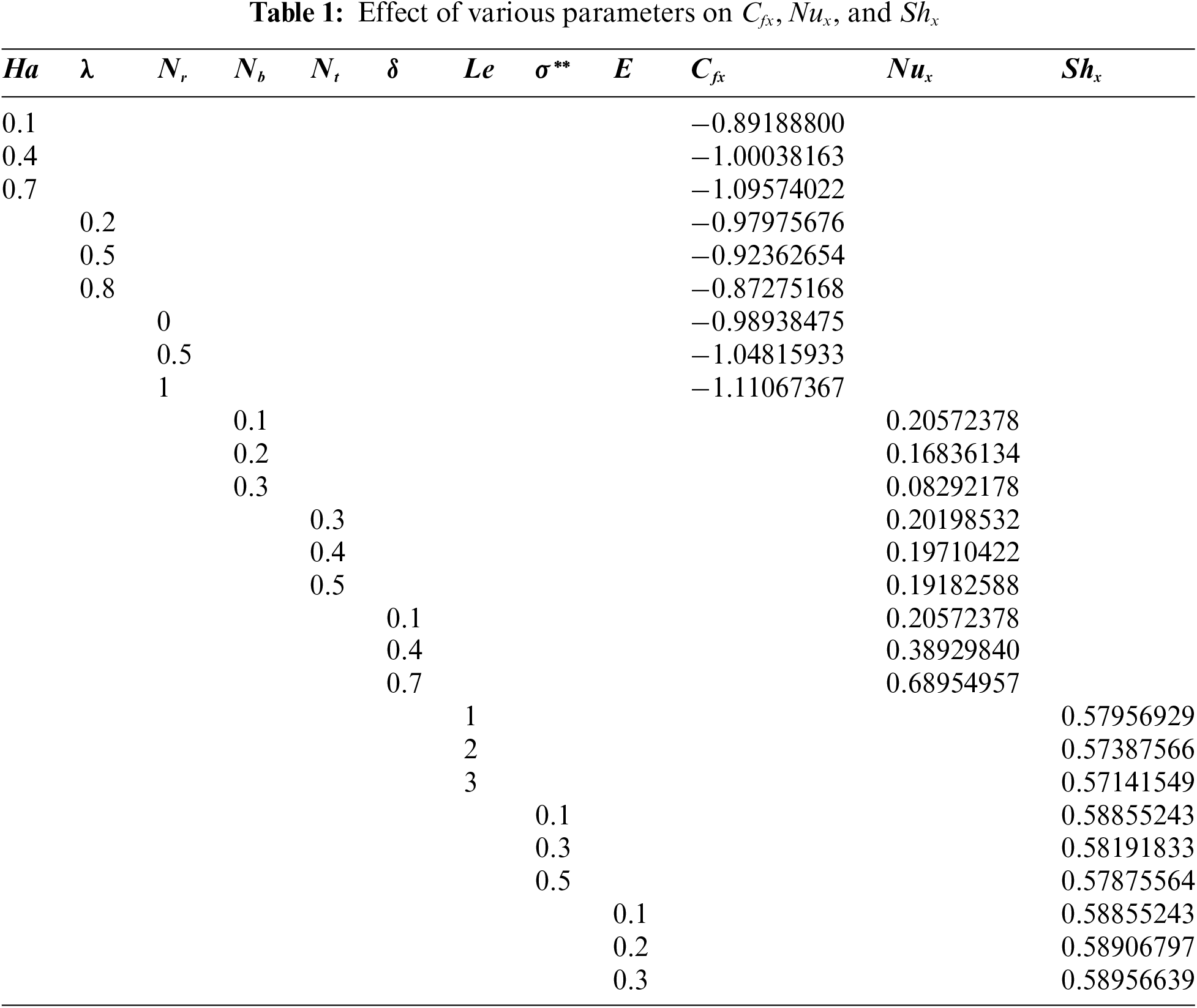
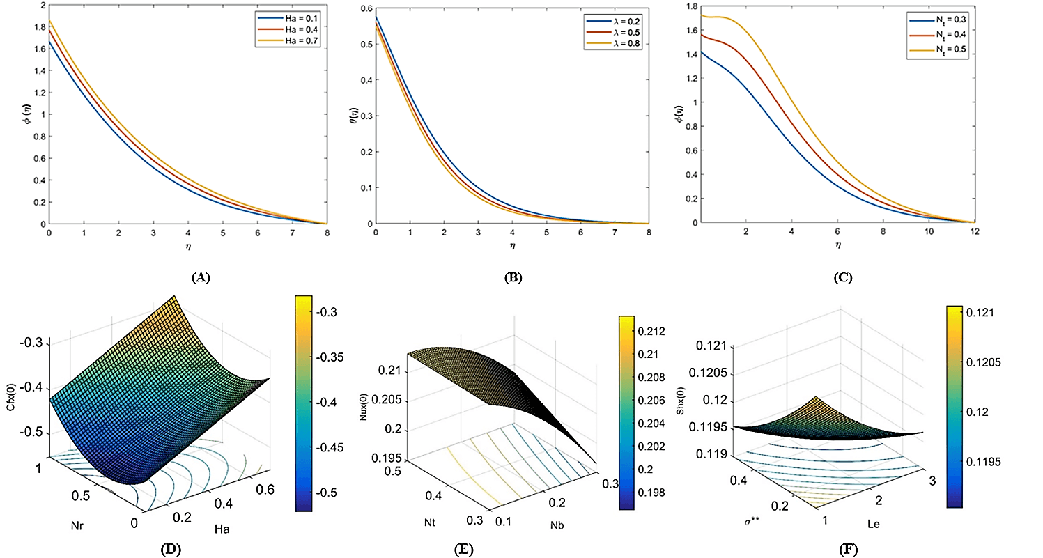
Fig. 1 presents the effect of

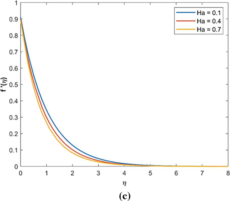
Figure 1: Ha effect. (a) Concentration profile against variation of
The effect of the mixed convective parameter

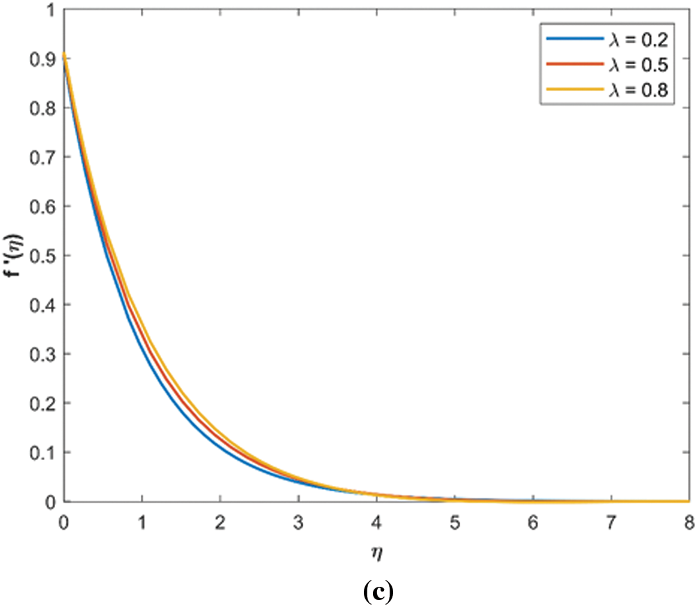
Figure 2: Mixed convective parameter effect (a) Concentration profile for variations in
The effect of

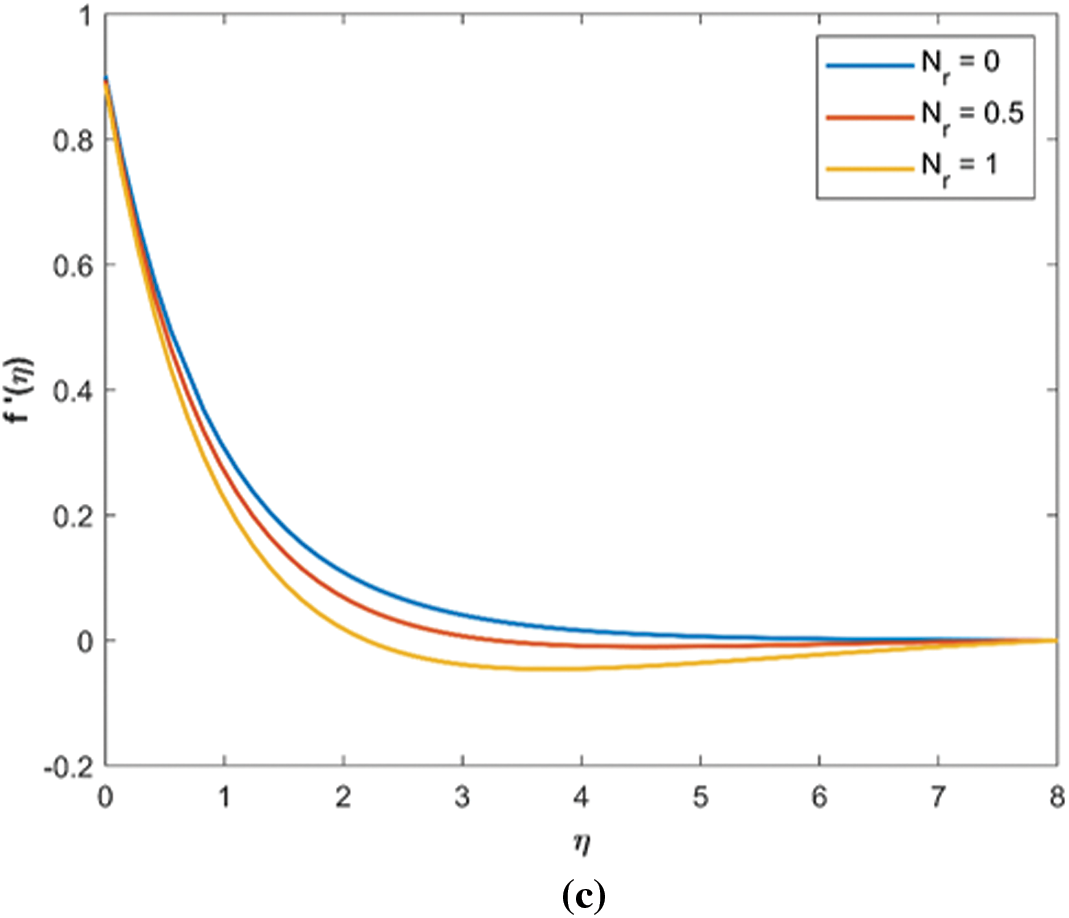
Figure 3:
Fig. 4 presents the impact of
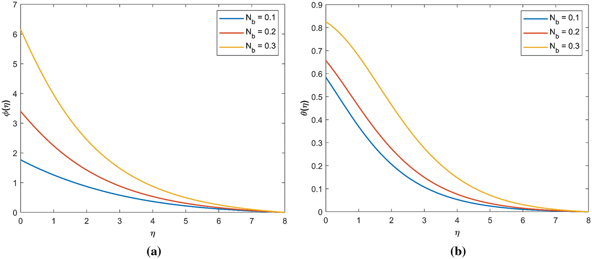
Figure 4: Nb effect. (a) Effect of
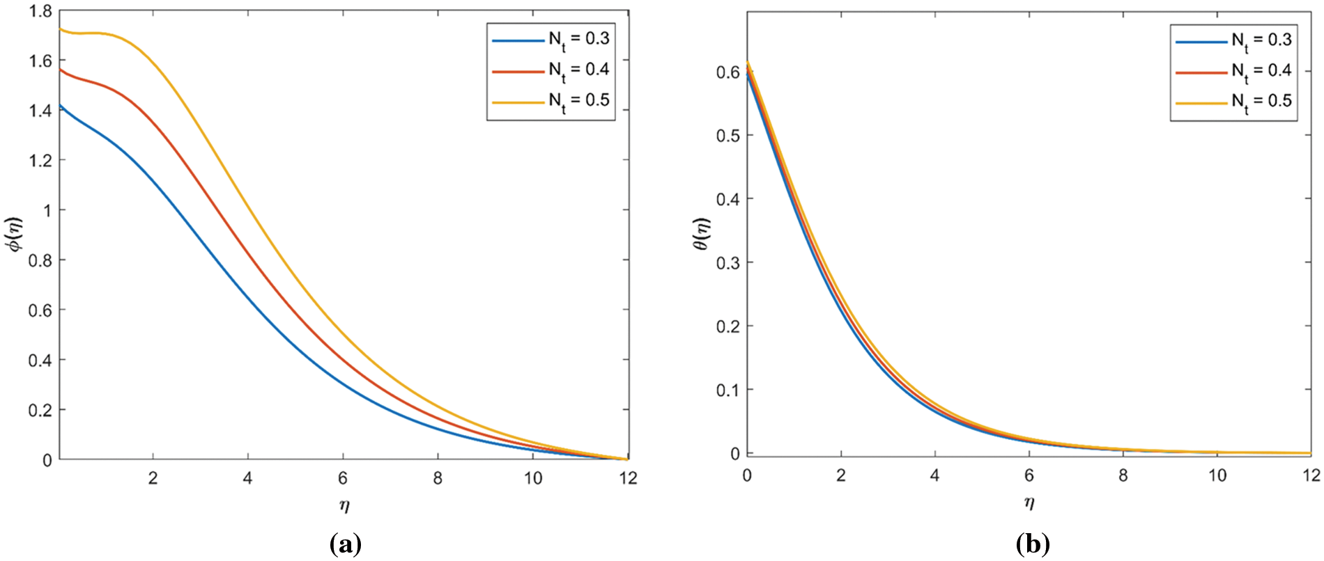
Figure 5: Nt effect. (a) Impact of
Fig. 6 is plotted to observe the impact of
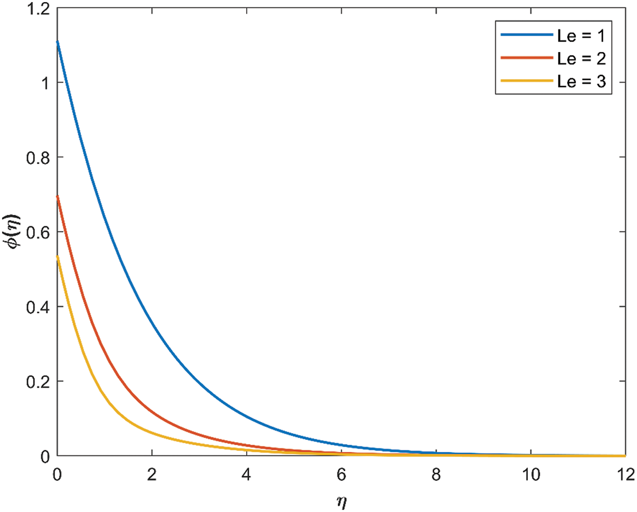
Figure 6: Effect of
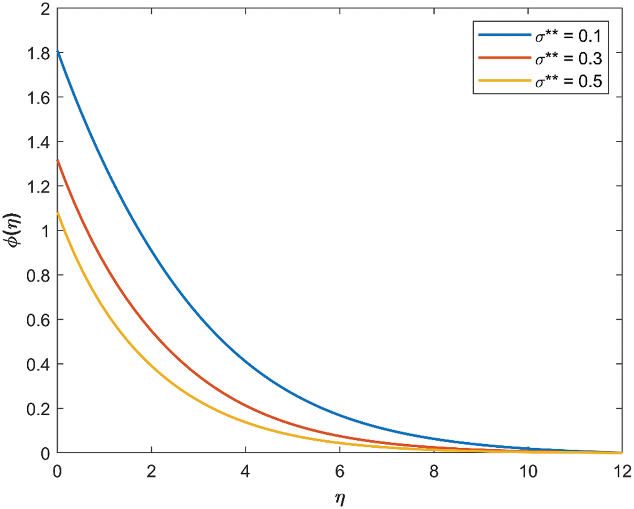
Figure 7: Effect of
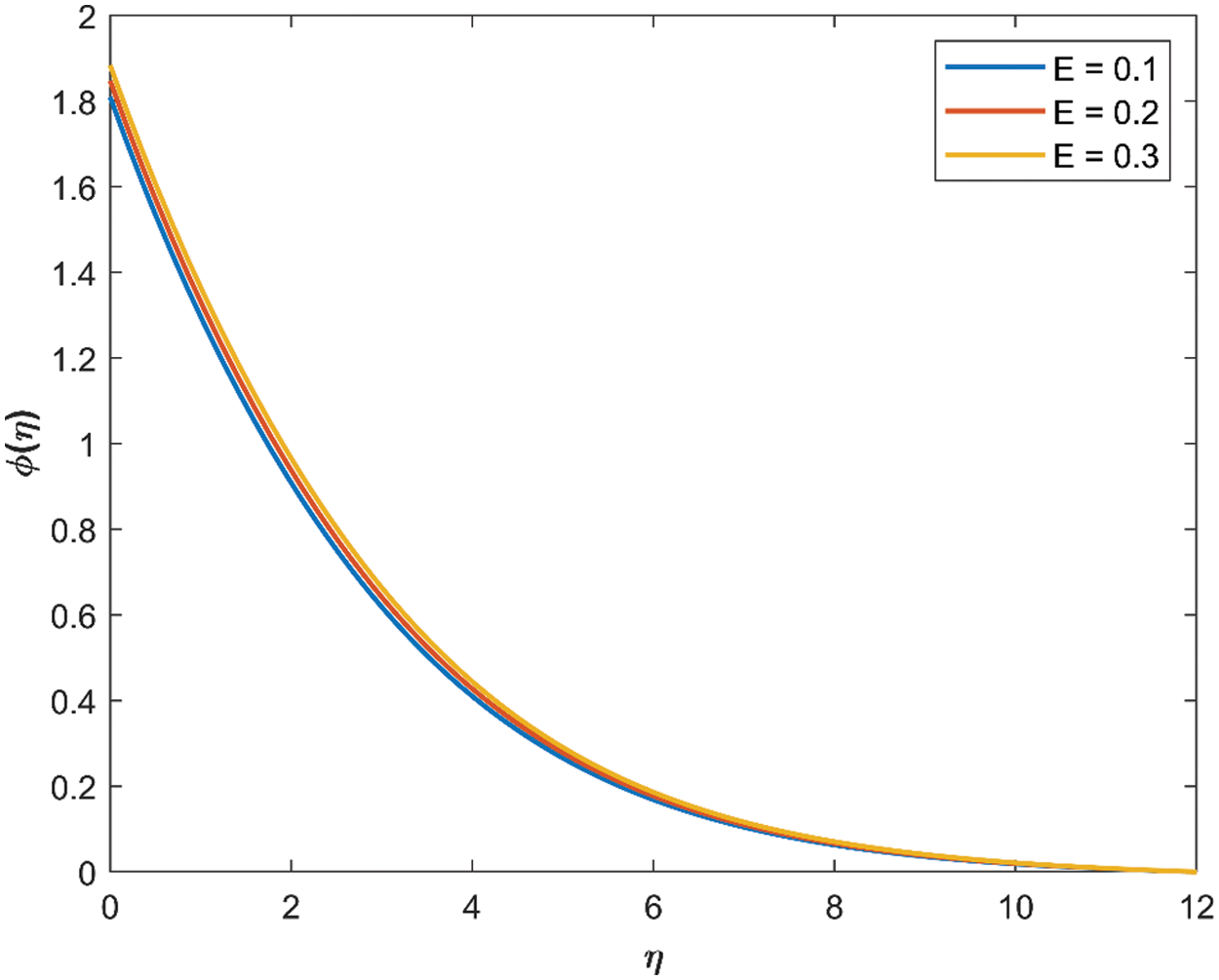
Figure 8: Effect of
RSM is a powerful tool to describe a broad range of variables, with partial resources, quantitative data, and the mandatory test design. The stages involved in RSM are as follows:
1. The investigation of data values is planned and executed to achieve appropriate and credible requirements for the projected response.
2. The most suitable mathematical models were described for the response surface.
3. It was defined that the mathematical models of the response surface are the most suitable.
4. To inspect the parametric direct and interaction impacts (ANOVA), variance analysis was done.
4.2 Optimization Analysis by RSM
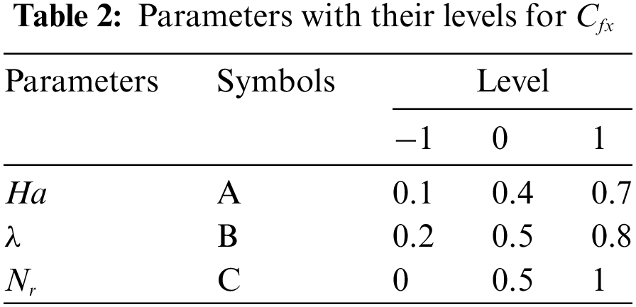
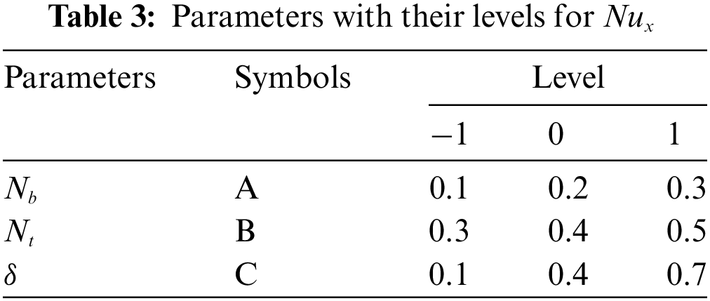
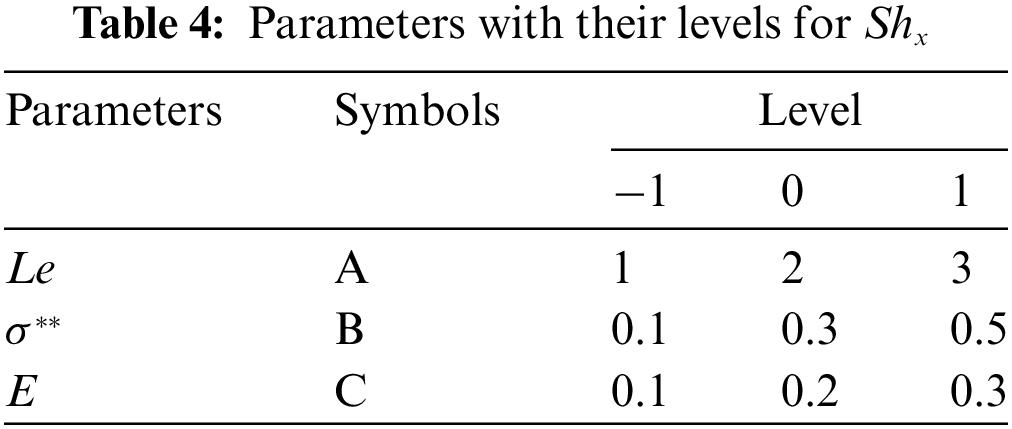
The relation among the response variable and factor variables was computed by employing a face-centered central composite design. Tables 2–4 describe the inclusive factors and levels. The model is described in (13), in which the linear, square, and interactive terms are involved.
Response =
4.2.1 Response Surface Regression:
This section examined the response of three factors
i) Statistical Analysis
Based on the given settings. The statistical analysis executed 20 runs for
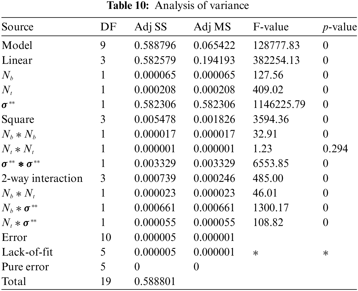
ii) Analysis of Variance and Model Estimation:
To achieve the projected regression equation, experimental model presented in Table 8 is executed under altered experimental settings. The residual plot is achieved by analysis of variance and entering the data into analytical software.
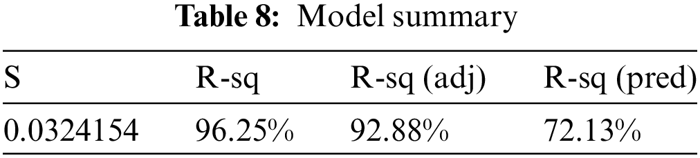
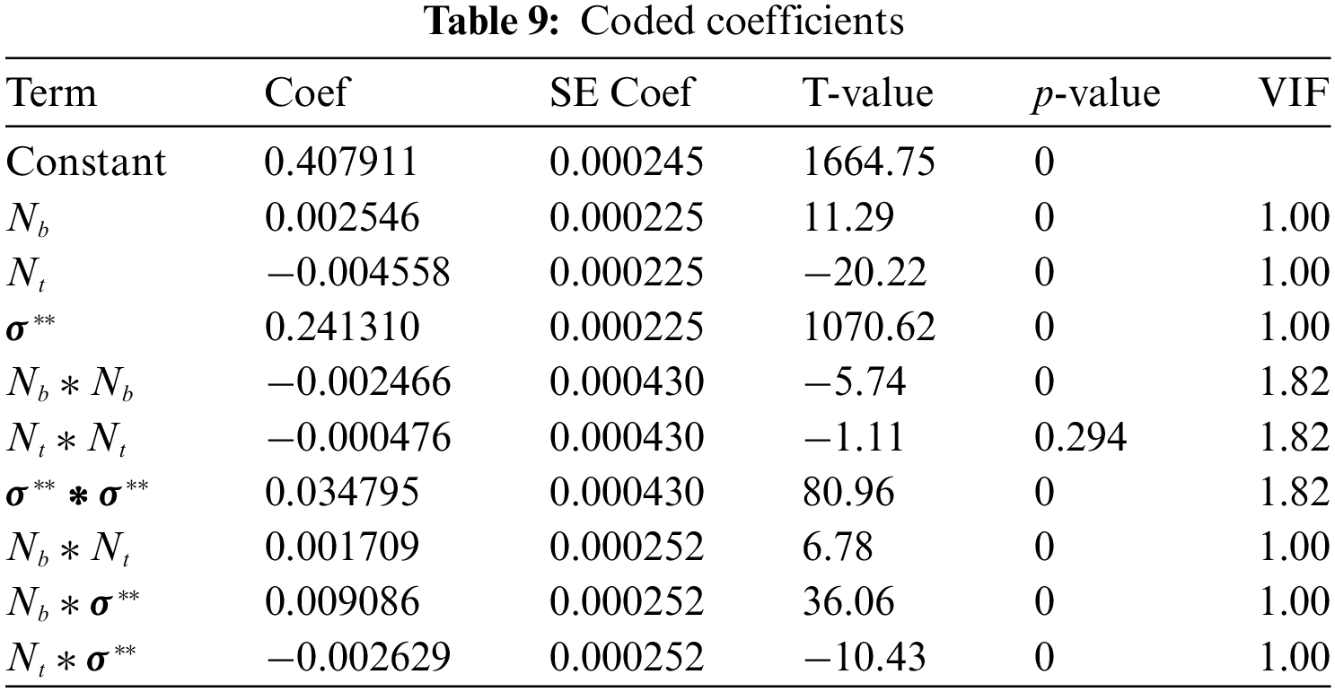
From Table 7, it is noticed that
iii) Regression Equation in Uncoded Units
From Table 8 it is noticed that the p-value of
After removing the factors which have a p-value greater than 0.05 the regression equation for
iv) Residual and Surface Plots
The residual plot is given in Fig. 9a. In the residual plot difference in observed
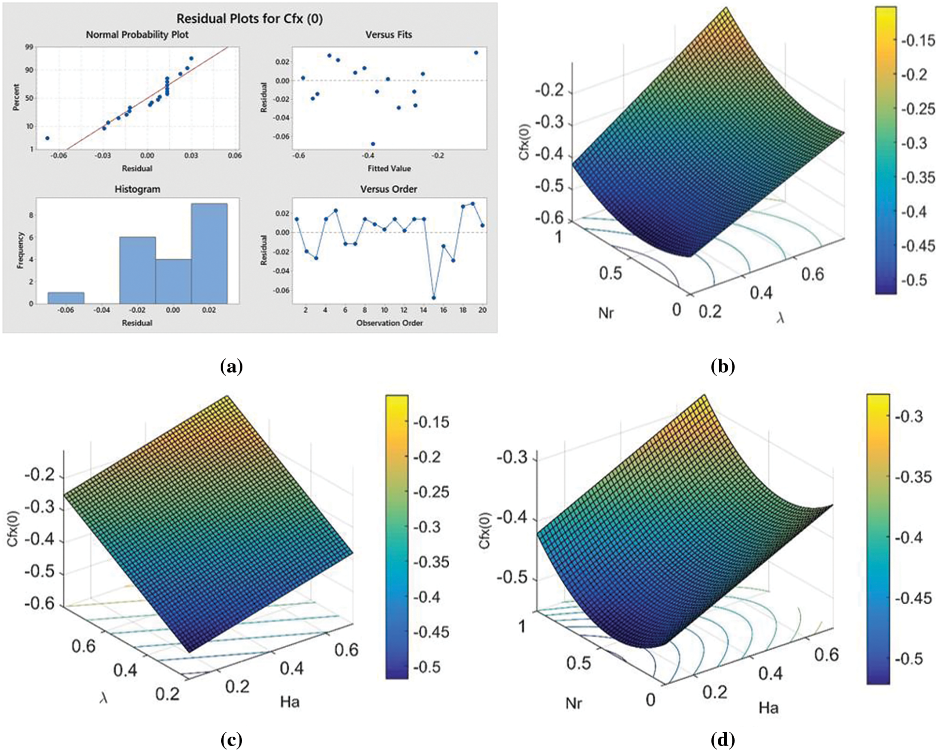
Figure 9: Influential factors on
Fig. 9b represents
Fig. 9c observed the influence of
4.2.2 Response Surface Regression:
In this section, the response of three factors
i) Statistical Analysis:
According to the given settings, the statistical analysis executed 20 runs for
ii) Analysis of Variance and Model Estimation:
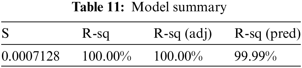
To get the approximate regression equation, the experimental model presented in Table 11 is executed under changed experimental settings. The residual plot is achieved by analysis of variance and entering the data into analytical software. By applying RSM we get Eq. (16) which is a frequent relationship between their valuable factors.
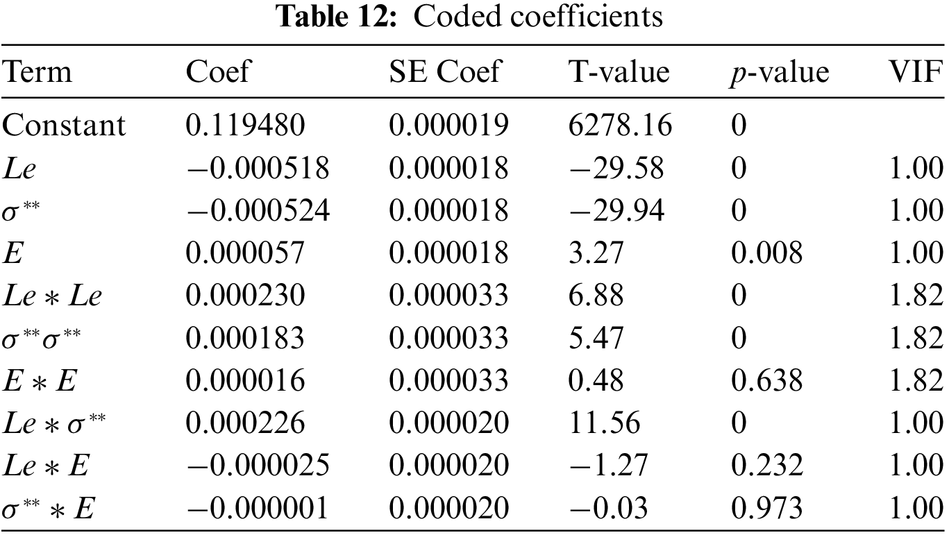
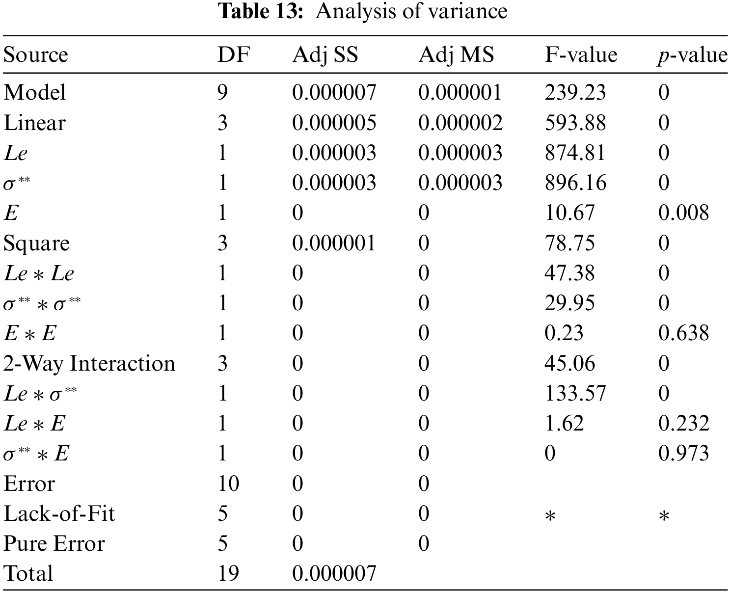
From Table 10, it is observed that the p-value of
iii) Regression Equation in Uncoded Units
From Table 11, it is observed that the p-value of
After eliminating the factors which have a p-value greater than 0.05 the regression equation for
iv) Residual and Surface Plots
The residual plot is given in Fig. 10a. In the residual plot difference observed from the scattered plot and predicted
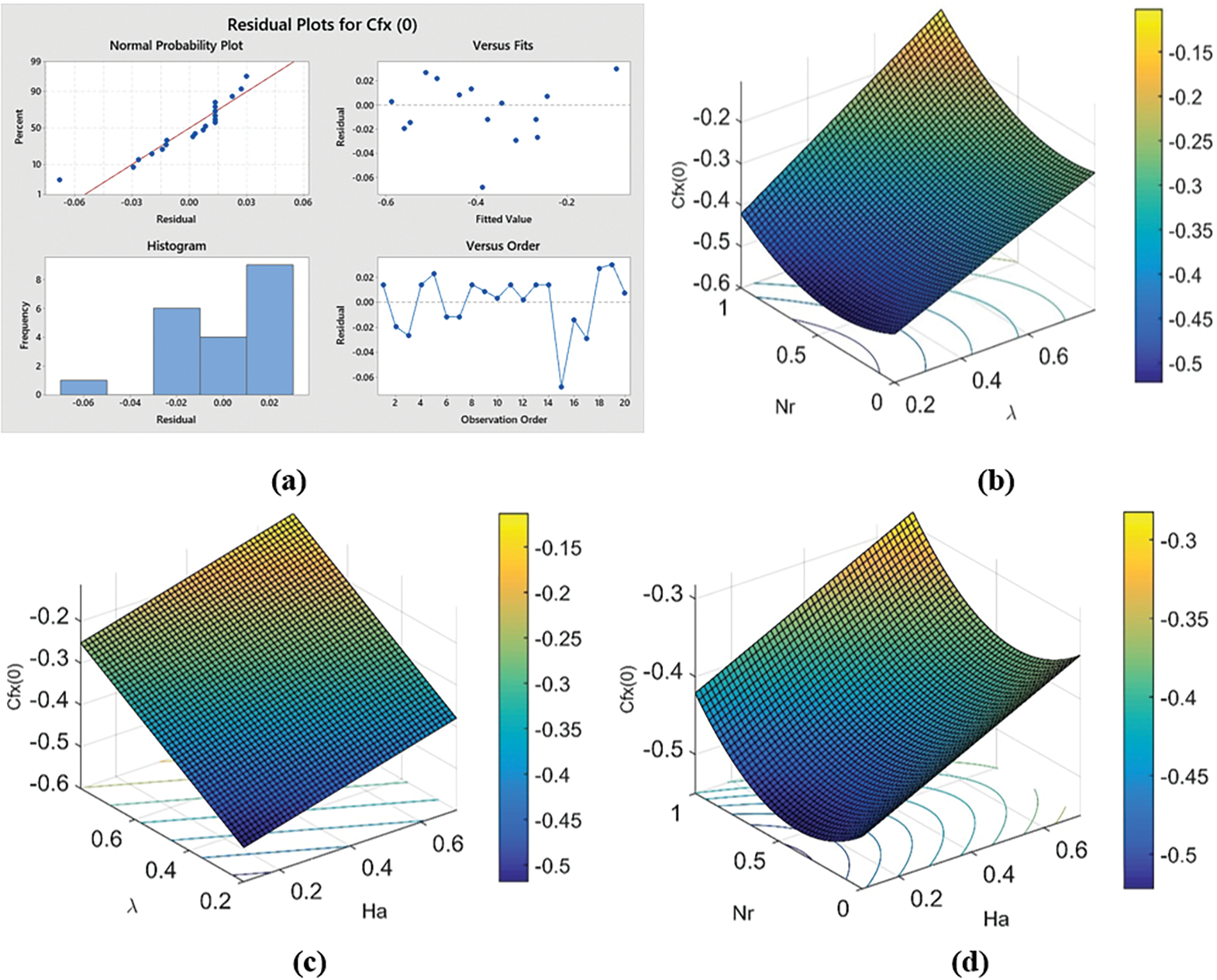
Figure 10: Influential factors on
4.2.3 Response Surface Regression:
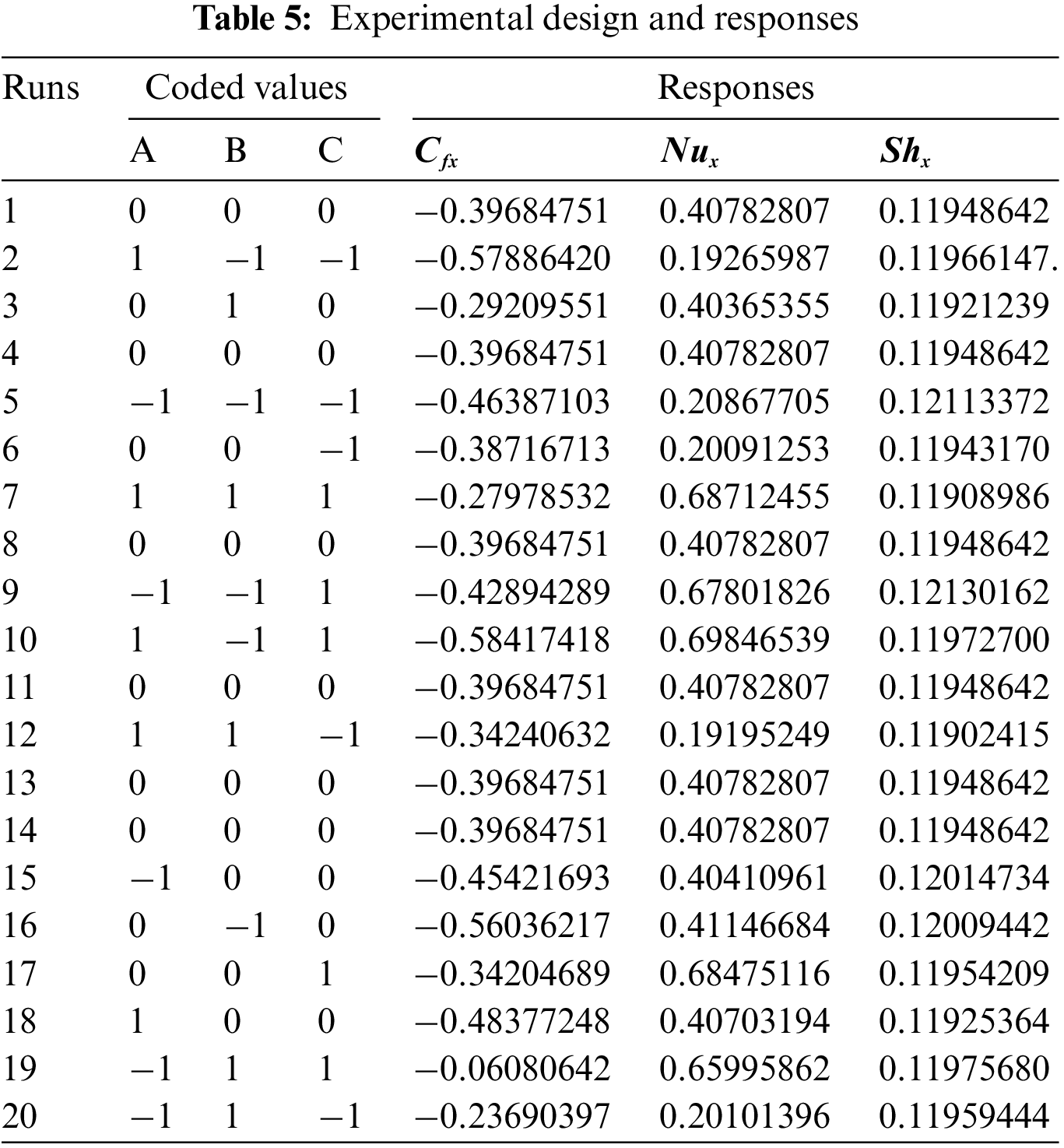
In this section, the response of three factors of
i) Statistical Analysis:
According to specified settings. The statistical analysis executed 20 runs for
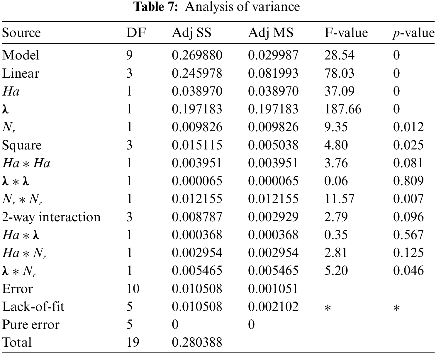
ii) Analysis of Variance and Model Estimation:
To get the approximate regression equation of the experimental model presented in Table 14 is executed under transformed experimental settings. The residual plot is achieved by analysis of variance and entering the data into analytical software. By using RSM we get Eq. (18) which is a numerous relationship between their helpful factors.
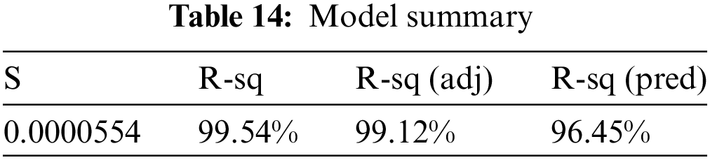
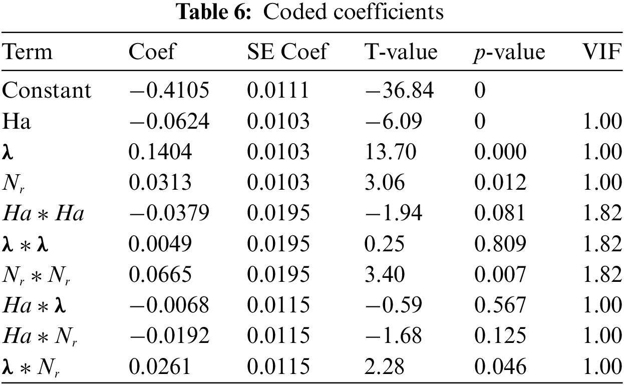
From Table 13 it is observed that the p-value of
iii) Regression Equation in Uncoded Units
From Table 14 it is observed that the p-value of
After eliminating the factors which have a p-value greater than 0.05 the regression equation for
iv) Residual and Surface Plots
The residual plot is given in Fig. 11a. In the residual plot difference observed from the scattered plot and predicted
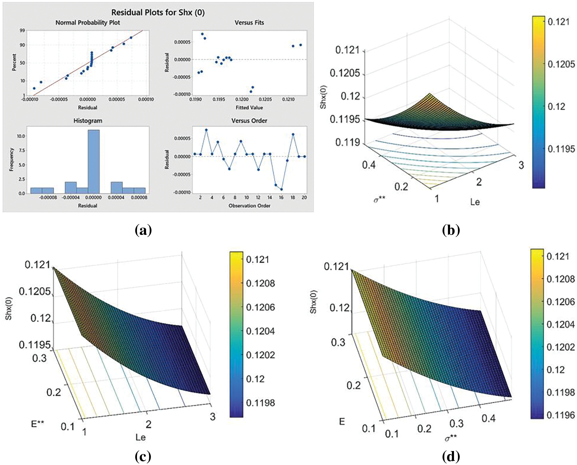
Figure 11: Influential factors on
In this study, the Casson nanofluid was examined, and its thermal analysis and optimizations were conducted. The following conclusions can be drawn:
• The velocity profile decreases with an increment in
• The temperature profile rises with enhancement in
• The concentration profile increases with rising values of
•
• For higher values of
• This work can be extended to hybrid and ternary hybrid nanofluids. Furthermore, the application of artificial neural networks could further optimize the study.
Acknowledgement: The authors express their gratitude to their affiliated universities.
Funding Statement: The authors received no specific funding for this study.
Author Contributions: The authors confirm their contribution to the paper as follows: study conception and design, data collection, analysis and interpretation of results, and draft manuscript preparation: Jawad Raza, F. Mebarek-Oudina, Haider Ali, I. E. Sarris. All authors reviewed the results and approved the final version of the manuscript.
Availability of Data and Materials: Data are available on request.
Conflicts of Interest: The authors certify that there are no conflicts of interest about the publication of this research.
References
1. Choi, S. U., Eastman, J. A. (1995). Enhancing thermal conductivity of fluids with nanoparticles (No. ANL/MSD/CP-84938; CONF-951135-29). Argonne, IL, USA: Argonne National Lab. (ANL). [Google Scholar]
2. Buongiorno, J. (2006). Convective transport in nanofluids. Journal of Heat Transfer, 128(3), 240–250. https://doi.org/10.1115/1.2150834 [Google Scholar] [CrossRef]
3. Sheikholeslami, M., Bhatti, M. M. (2017). Forced convection of nanofluid in presence of constant magnetic field considering shape effects of nanoparticles. International Journal of Heat and Mass Transfer, 111(7), 1039–1049. https://doi.org/10.1016/j.ijheatmasstransfer.2017.04.070 [Google Scholar] [CrossRef]
4. Ahmed, J., Khan, M., Ahmad, L. (2019). Stagnation point flow of Maxwell nanofluid over a permeable rotating disk with heat source/sink. Journal of Molecular Liquids, 287(9), 110853. https://doi.org/10.1016/j.molliq.2019.04.130 [Google Scholar] [CrossRef]
5. Imtiaz, M., Hayat, T., Alsaedi, A., Ahmad, B. (2016). Convective flow of carbon nanotubes between rotating stretchable disks with thermal radiation effects. International Journal of Heat and Mass Transfer, 101(1), 948–957. https://doi.org/10.1016/j.ijheatmasstransfer.2016.05.114 [Google Scholar] [CrossRef]
6. Garoosi, F., Jahanshaloo, L., Rashidi, M. M., Badakhsh, A., Ali, M. E. (2015). Numerical simulation of natural convection of the nanofluid in heat exchangers using a Buongiorno model. Applied Mathematics and Computation, 254, 183–203. https://doi.org/10.1016/j.amc.2014.12.116 [Google Scholar] [CrossRef]
7. Sheikholeslami, M., Ganji, D. D., Rashidi, M. M. (2016). Magnetic field effect on unsteady nanofluid flow and heat transfer using Buongiorno model. Journal of Magnetism and Magnetic Materials, 416(45), 164–173. https://doi.org/10.1016/j.jmmm.2016.05.026 [Google Scholar] [CrossRef]
8. Mustafa, M. (2017). MHD nanofluid flow over a rotating disk with partial slip effects: Buongiorno model. International Journal of Heat and Mass Transfer, 108, 1910–1916. https://doi.org/10.1016/j.ijheatmasstransfer.2017.01.064 [Google Scholar] [CrossRef]
9. Turkyilmazoglu, M. (2018). Buongiorno model in a nanofluid filled asymmetric channel fulfilling zero net particle flux at the walls. International Journal of Heat and Mass Transfer, 126, 974–979. https://doi.org/10.1016/j.ijheatmasstransfer.2018.05.093 [Google Scholar] [CrossRef]
10. Dharmaiah, G., Mebarek-Oudina, F., Balamurugan, K. S., Vedavathi, N. (2024). Numerical analysis of the magnetic dipole effect on a radiative ferromagnetic liquid flowing over a porous stretched sheet. Fluid Dynamics & Materials Processing, 20(2), 293–310.https://doi.org/10.32604/fdmp.2023.030325 [Google Scholar] [CrossRef]
11. Sheikholeslami, M., Rokni, H. B. (2017). Effect of melting heat transfer on nanofluid flow in existence of magnetic field considering Buongiorno Model. Chinese Journal of Physics, 55(4), 1115–1126. https://doi.org/10.1016/j.cjph.2017.04.019 [Google Scholar] [CrossRef]
12. Tsuji, Y., Morikawa, Y., Tanaka, T., Nakatsukasa, N., Nakatani, M. (1987). Numerical simulation of gas-solid two-phase flow in a two-dimensional horizontal channel. International Journal of Multiphase Flow, 13(5), 671–684. https://doi.org/10.1016/0301-9322(87)90044-9 [Google Scholar] [CrossRef]
13. Hieu, P. D., Katsutoshi, T., Ca, V. T. (2004). Numerical simulation of breaking waves using a two-phase flow model. Applied Mathematical Modelling, 28(11), 983–1005. [Google Scholar]
14. Zeidan, D., Romenski, E., Slaouti, A., Toro, E. F. (2007). Numerical study of wave propagation in compressible two-phase flow. International Journal for Numerical Methods in Fluids, 54(4), 393–417. [Google Scholar]
15. Ljungqvist, M., Rasmuson, A. (2001). Numerical simulation of the two-phase flow in an axially stirred vessel. Chemical Engineering Research and Design, 79(5), 533–546. [Google Scholar]
16. Xue, Y., Liu, J., Liang, X., Wang, S., Ma, Z. (2022). Ecological risk assessment of soil and water loss by thermal enhanced methane recovery: Numerical study using two-phase flow simulation. Journal of Cleaner Production, 334, 130183. [Google Scholar]
17. Huang, Z., Yao, J., Wang, Y., Tao, K. (2011). Numerical study on two-phase flow through fractured porous media. Science China Technological Sciences, 54, 2412–2420. [Google Scholar]
18. Riaz, A., Tchelepi, H. A. (2006). Numerical simulation of immiscible two-phase flow in porous media. Physics of Fluids, 18(1), 014104. [Google Scholar]
19. Rana, P., Bhargava, R. (2012). Flow and heat transfer of a nanofluid over a nonlinearly stretching sheet: A numerical study. Communications in Nonlinear Science and Numerical Simulation, 17(1), 212–226. [Google Scholar]
20. Mabood, F., Khan, W. A., Ismail, A. M. (2015). MHD boundary layer flow and heat transfer of nanofluids over a nonlinear stretching sheet: A numerical study. Journal of Magnetism and Magnetic Materials, 374, 569–576. [Google Scholar]
21. Nadeem, S., Haq, R. U., Khan, Z. H. (2014). Numerical study of MHD boundary layer flow of a Maxwell fluid past a stretching sheet in the presence of nanoparticles. Journal of the Taiwan Institute of Chemical Engineers, 45(1), 121–126. [Google Scholar]
22. Pattnaik, P. K., Mishra, S. R., Barik, A. K., Mishra, A. K. (2020). Influence of chemical reaction on magnetohydrodynamic flow over an exponential stretching sheet: A numerical study. International Journal of Fluid Mechanics Research, 47(3), 217–228. [Google Scholar]
23. Narayana, P. S., Babu, D. H. (2016). Numerical study of MHD heat and mass transfer of a Jeffrey fluid over a stretching sheet with chemical reaction and thermal radiation. Journal of the Taiwan Institute of Chemical Engineers, 59, 18–25. [Google Scholar]
24. Hayat, T., Saif, R. S., Ellahi, R., Muhammad, T., Ahmad, B. (2017). Numerical study of boundary-layer flow due to a nonlinear curved stretching sheet with convective heat and mass conditions. Results in Physics, 7, 2601–2606. [Google Scholar]
25. Mebarek-Oudina, F., Preeti, P., Sabu, A. S., Vaidya, H., Lewis, R. W. et al. (2024). Hydromagnetic flow of magnetite-water nano-fluid utilizing adapted Buongiorno model. International Journal of Modern Physics B, 38(1), 2450003. https://doi.org/10.1142/S0217979224500036 [Google Scholar] [CrossRef]
26. Mahanthesh, B., Gireesha, B. J., Gorla, R. S., Makinde, O. D. (2018). Magnetohydrodynamic three-dimensional flow of nanofluids with slip and thermal radiation over a nonlinear stretching sheet: A numerical study. Neural Computing and Applications, 30, 1557–1567. [Google Scholar]
27. Ramesh, K., Mebarek-Oudina, F., Ismail, A. I., Jaiswal, B. R., Warke, A. S. et al. (2023). Computational analysis on radiative non-Newtonian Carreau nanofluid flow in a microchannel under the magnetic properties. Sciencia Iranica, 30(2), 376–390. [Google Scholar]
28. Ali, A., Mebarek-Oudina, F., Barman, A., Das, S., Ismail, A. I. (2023). Peristaltic transportation of hybrid nano-blood through a ciliated micro-vessel subject to heat source and Lorentz force. Journal of Thermal Analysis and Calorimetry, 148(14), 7059–7083. https://doi.org/10.1007/s10973-023-12217-x [Google Scholar] [CrossRef]
29. Li, S., Faizan, M., Ali, F., Ramasekhar, G., Muhammad, T. et al. (2024). Modelling and analysis of heat transfer in MHD stagnation point flow of Maxwell nanofluid over a porous rotating disk. Alexandria Engineering Journal, 91(4), 237–248. https://doi.org/10.1016/j.aej.2024.02.002 [Google Scholar] [CrossRef]
30. Khan, N., Ali, F., Ahmad, Z., Murtaza, S., Ganie, A. H. et al. (2023). A time fractional model of a Maxwell nanofluid through a channel flow with applications in grease. Scientific Reports, 13(1), 4428. https://doi.org/10.1038/s41598-023-31567-y. [Google Scholar] [PubMed] [CrossRef]
31. Khan, M. N., Ahmad, S., Alrihieli, H. F., Wang, Z., Hussien, M. A. et al. (2023). Theoretical study on thermal efficiencies of Sutterby ternary-hybrid nanofluids with surface catalyzed reactions over a bidirectional expanding surface. Journal of Molecular Liquids, 391(10), 123412. https://doi.org/10.1016/j.molliq.2023.123412 [Google Scholar] [CrossRef]
32. Bejawada, S. G., Nandeppanavar, M. M. (2023). Effect of thermal radiation on magnetohydrodynamics heat transfer micropolar fluid flow over a vertical moving porous plate. Experimental and Computational Multiphase Flow, 5(2), 149–158. https://doi.org/10.1007/s42757-021-0131-5 [Google Scholar] [CrossRef]
33. Mebarek-Oudina, F., Chabani, I., Vaidya, H., Ismail, A. I. (2024). Hybrid nanofluid magnetoconvective flow and porous media contribution to entropy generation. International Journal of Numerical Methods for Heat & Fluid Flow, 33(1), 2540003. https://doi.org/10.1108/HFF-06-2023-0326 [Google Scholar] [CrossRef]
34. Mabood, F., Khan, S. U., Tlili, I. (2023). Numerical simulations for swimming of gyrotactic microorganisms with Williamson nanofluid featuring Wu’s slip, activation energy and variable thermal conductivity. Applied Nanoscience, 13(5), 131–144. https://doi.org/10.1007/s13204-020-01548-y [Google Scholar] [CrossRef]
35. Ijaz Khan, M., Alzahrani, F. (2020). Activation energy and binary chemical reaction effect in nonlinear thermal radiative stagnation point flow of Walter-B nanofluid: Numerical computations. International Journal of Modern Physics B, 34(13), 2050132. https://doi.org/10.1142/S0217979220501325 [Google Scholar] [CrossRef]
36. Ramesh, K., Mebarek-Oudina, F., Souayeh, B. (2023). Mathematical modelling of fluid dynamics and nanofluids, 1st edition. CRC Press (Taylor & Francis). https://doi.org/10.1201/9781003299608 [Google Scholar] [CrossRef]
Cite This Article
 Copyright © 2024 The Author(s). Published by Tech Science Press.
This work is licensed under a Creative Commons Attribution 4.0 International License , which permits unrestricted use, distribution, and reproduction in any medium, provided the original work is properly cited.
 Downloads
 Citation Tools