Reducing Condensation Inside the Photovoltaic (PV) Inverter according to the Effect of Diffusion as a Process of Vapor Transport

1  Introduction

Batteries, a meter, inverters, and solar panels are used to construct solar power systems. Low-maintenance solar PV systems continue to be such as long as they are installed correctly. The solar panels produce the electricity, and the solar inverters transform the DC electricity into AC electricity to provide power to the buildings. Compared to solar panels, inverters have a lot more electrical components and are far more prone to malfunction. Microinverters can endure for twenty to twenty-five years, while string solar inverters have a lifespan of ten to fifteen years. Even though inverters are supposed to endure for decades, a number of things can interfere with their performance, like heat, improper installation, humidity, and poor maintenance. Life data analysis involves the statistical analysis of historical data to develop mathematical models that describe behavior (reliability and maintainability). Several powerful computer processors, a variety of artificial intelligent (AI) algorithms, computer codes, and simulation software may make up the AI platform, according to [1,2]. The heating, cooling, and lighting systems of a building should be very energy-efficient and adaptable, and the features and qualities of the main elements of an EFB should be highly customizable in order to fully benefit from AI. Gas furnaces that are 95% efficient have grown in popularity recently, and micro-CHP (Combined Heat and Power) systems have been offered commercially for a while. For more details, see [3].

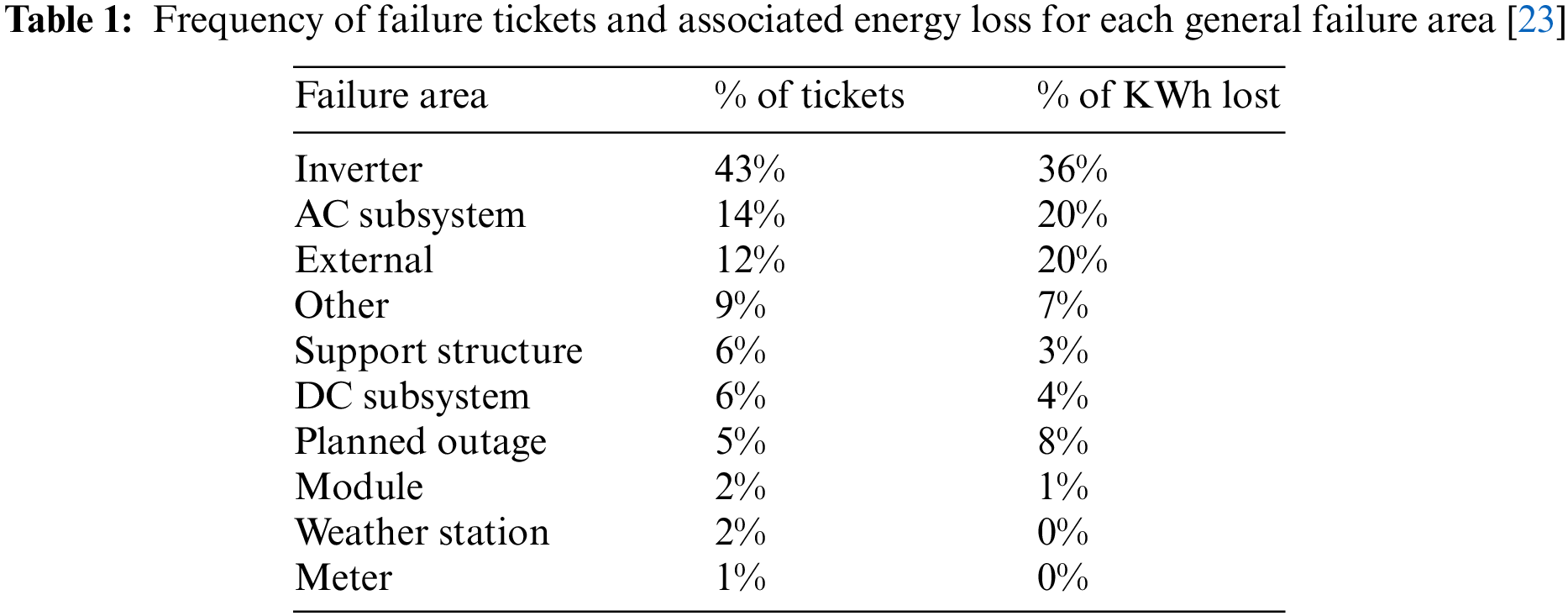
The statistical models used are distributions or stochastic process models. The most commonly used distributions are Weibull [4], Lognormal [5], Exponential [6], and Weibull-Bayesian [7]. After executing the models, the outcomes were compared to the criteria established for success and failure using statistical techniques such as Weibull analysis. Next, the findings and outcomes were documented and analyzed, taking into account assumptions and any limitations of the results to assist researchers in choosing the best algorithm for designing the prediction model with better accuracy [4–7]. Estimate the solar radiation at different locations across different climatic conditions and find the ideal locations for the construction of solar power stations. The predictive model can aid decision-makers in modeling and planning solar systems, particularly in designing photovoltaic systems. A predictive development model can be highly used to use routine meteorological parameters as inputs to overcome the lack of a solar radiation database in remote regions where measuring instruments are not available [8–10]. Each analytical technique has its own set of requirements based on its fit with the current research understudy’s objectives, data input and transformation requirements, and output evaluation and deployment based on the study [11]. While the number of analytical techniques continues to rise, it is critical to have a formalized knowledge discovery approach that incorporates all applicable analytical techniques for a specific environmental risk management challenge. The data analytics life cycle approach incorporates this requirement and expands on current data mining techniques developed by [12,13]. Analytical application developers and implementers can utilize data analytics as a research lens that focuses on issues that are pertinent to them [14]. After executing the model, the outcomes are compared to the criteria established for success and failure using statistical techniques such as ANOVA [15]. According to the studies [16,17], the grid-connected PV inverter is the least reliable of the bunch because of the power semiconductor switches. The dependability of PV inverters is influenced by factors including quality control, sufficient design, electrical component failure, and other manufacturing concerns. Any grid-tied solar system’s most complex component, the solar inverter, is also, regrettably, the component most prone to experiencing problems. This should not come as a surprise because inverters are typically installed outside in inclement weather, such as rain, humidity, and excessive heat, while producing thousands of watts of power for up to 10 h each day. This is why it’s crucial to use a high-quality inverter and, if feasible, put it in a protected area. Find out more about locating solar system faults. Reliability forecasts presuppose that a system failure brought on by stress or deprived manufacturing will be caused by one of the electronics components. The typical lifespan of string solar inverters is less than 15 years, which is 10 years fewer than the typical lifespan of solar panels. Inverters can live up to 20 years with proper maintenance and inspections, according to [18–21]. Examination of the relationship between operational reliability evaluation of PV inverters and power system reliability, as well as the impact of relative humidity on these relationships. It has been demonstrated through numerical examples that relative humidity has a significant impact on how reliable PV inverters are operating. Furthermore, it is impossible to ignore how PV inverters’ operational reliability affects the power system’s reliability. A bottom-up method for “relative humidity-components-PV inverters-power system” reliability evaluation is investigated in the study of [22]. The most frequent cause of solar inverter failures cannot be determined from the available data. Various kinds of electronic components, each with a varying failure rate, are used in residential and commercial string inverters. The frequency of failure reasons for each generic failure is displayed. Other reasons, such as humidity, are also taken into account. If any component of the electronic device is exposed to moist air or condensation, there is a risk of damage. Given the moisture content of the air, saturation occurs when the temperature drops to the dew point, which can lead to condensation on surfaces. However, the failures could also be attributed to hardware components since there was no investigation beyond restarting the inverter, according to the following table.

The data in Table 1 indicates that PV inverter failures constitute the highest percentage of failures in PV systems. So, the next study examines the effects of condensation as a factor in solar inverter function failure and finds a method for decreasing vapor condensation inside the photovoltaic (PV) inverter under the influence of external wind speed on diffusion, such as a method of moving moister air outside the inverter box as shown in [23]. The model employed in reliability evaluation techniques for PV systems today is oversimplified, and it ignores the effect that variations in the system’s thermal environment have on component attenuation and system dependability. Because of the limitations of the empirical test of PV inverter dependability, it is primarily based on long-term operational data. For thorough analysis and evaluation during PV inverter operation, taking into account the environmental variables at the site [24]. This study evaluates and handles one of the most important causes of a photovoltaic (PV) inverter’s failure. A photovoltaic (PV) inverter is an essential component of any photovoltaic (PV) solar system. Photovoltaic (PV) inverter failure can indicate that a solar system is no longer functional. Electronic devices, such as photovoltaic (PV) inverters, are exposed to vapor condensation. Given the amount of moisture in the air, saturation occurs when the temperature drops to the dew point, causing condensation to develop on surfaces. Numerical simulation with “COMSOL Software” is vital for acquiring knowledge about preventing condensation in two steps. To determine the amount of liquid water accumulated on the internal walls of the photovoltaic (PV) inverter box, the device’s water vapor concentration was first assumed to be homogeneous. Second, investigate the effect of external wind velocity on moisture transport at the air interface in order to assess water vapor transfer outside and reduce condensation. General factorial designs are used to investigate the nature of the relationship between vapor condensation response and variables.

2  Numerical Model

2.1 Model Definitions

Numerical simulations were solved with “COMSOL Software,” which can be used to learn information about condensation prevention. Changes in the air’s properties are the main source of condensation in various systems. Determine whether saturation happens when environmental factors vary by simulating the thermodynamic evolution of wet air in an electrical box. The air temperature, pressure, and relative humidity are calculated by the model using meteorological information. The location of the box is constantly shifting. This implies that during the simulation, changes in temperature, pressure, and water vapor concentration all occur. The information provided is consistent with a storm with a reduction in pressure. Damage to electronic devices always happens when exposed to humidity. When the temperature dips to the dew point and there is enough moisture in the air, saturation occurs, and condensation may start to develop on surfaces. To find out if condensation occurs when the ambient conditions outside the solar inverter box change, certain basic hypotheses are employed to simulate the thermodynamic evolution of moist air inside the enclosure. The model imports measured information for air pressure, temperature, and water vapor content. The concentration of water vapor inside the box is believed to be nonhomogeneous. The transport and diffusion of water vapors are under investigation. At first, the purpose of this simulation is to assume that the internal water vapor concentration is constant and equal to the external concentration. Additionally, during the simulation, the model design accounts for variations in external concentration while ignoring diffusion. Interpolation functions of temperature, normal stress, and relative humidity with time [T_ext (t) (K), p_ext (t), and c_ext (t)] are determined as shown in Fig. 1a–c. In the second simulation, the vapor concentration is calculated using a convection-diffusion equation with a diffusion coefficient of 2.5 10−5 m2/s. By establishing an open boundary condition with a specified time-dependent external concentration, one can lessen vapor condensation by detecting the influence of transport as a diffusion process.

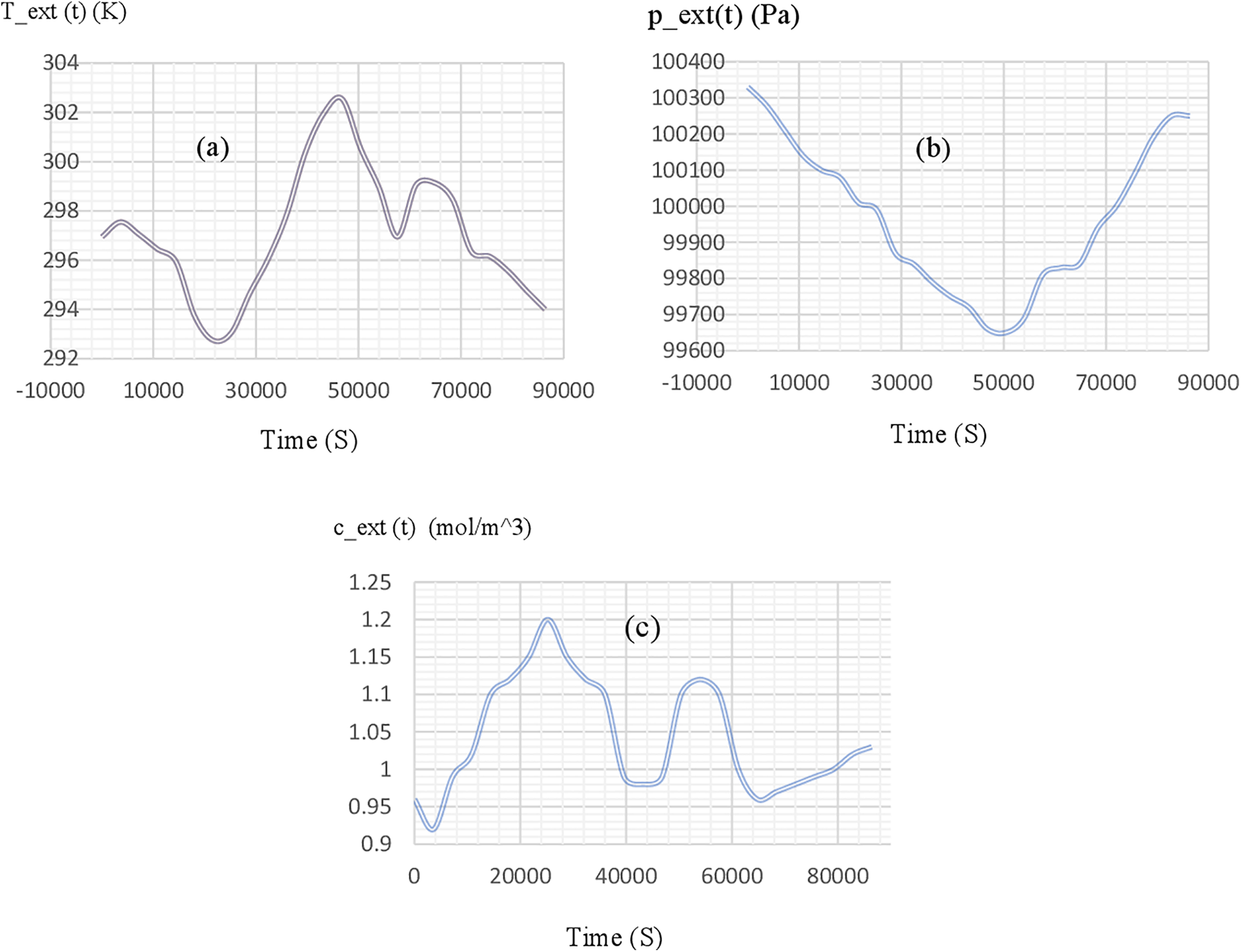
Figure 1: Interpolation functions of time temperature, normal stress and relative humidity of a day

2.2 Conjugate Heat Transfer

Conjugate heat transfer experiments have been carried out in the past by numerous researchers for a variety of purposes. When considering the answer to the heat transfer problem, in which heat dissipation happens in a fluid flow that surrounds a solid source of heat generation, “conjugate heat transfer,” Heat conduction equations that apply to both fluids and solids were taken into consideration in this study to get asymptotic solutions to integral equations. The majority of these early investigations centered on the heat exchange between a solid plate and the fluid surrounding it. With the use of presumptive thermal boundary layer velocity profiles, various analytical solutions were put forth. Continuity, momentum, equations for fluids, and the two-dimensional heat conduction equation for solids served as the basic foundation for these early two-dimensional researches [25,26]. These equational systems can be written as:

ρ∂u∂t+ρ(u.∇)u=∇.[−ρI+µ(∇u+(∇u)T)−23μ(∇.u)I]+F(1)

ρ  the (mass) density (kg/m3)

u  velocity vector (m/s)

∇  divergence,

I   heat flux (W/m2)

t   time, S

F   Body force vector (N/m3)

Eq. (2), often known as the general continuity equation, is a result of mass conservation. Keep in mind that this is true regardless of whether a fluid is compressible or not.

∂ρ∂t+∇.(ρ)=0(2)

By convection of internal energy, thermal conduction, radiation, dissipation of mechanical stress, and extra volumetric heat sources, it is meant that fluctuations of internal energy over time are balanced. Eq. (3) will be derived in the parts that follow to produce the heat transport equations in various mediums.

ρcp∂T∂t+ρcPu.∇T=∇.(k∇T)+Q(3)

cP  Specific heat capacity at constant pressure (J/(kg·K))

T  Temperature (K)

k  Evaporation rate factor (m/s)

Q  Heat source (W/m3)

The following equation, which is derived from Eq. (3), is solved by the heat transfer in solids interface:

ρcp∂T∂t+ρcpu.∇T=∇.(K∇T)+Q(4)

Thermal Insulation

−n.(−k∇T)=0(5)

n Normal vector to ward exterior (dimensionless) at wall

u=0

In thermal convection, thermal diffusion by the random motion of the molecules and enthalpy flow by the bulk motion of the fluid combine to produce the energy transport through the aggregates (many molecules are moving collectively). Convection is utilized to describe this superposing transport, unless otherwise stated in this study, and advection to describe transport brought on by the fluid’s macroscopic motion [25,26]. For an incompressible fluid, the cartesian xi component of the overall convective heat flow q (= qx1, qx2, qx3 = qx and qy) may be represented using the unified heat flux formula of thermal convection [24,25]. Three contributions to the heat equation are made because of fluid motion:

I.   The movement of fluid also involves the movement of energy, which is represented by the convective contribution in the heat equation. Either convective heat transfer or conductive heat transfer may predominate, depending on the fluid’s thermal characteristics and the flow regime.

II.   Fluid heating is a result of the viscous effects of the fluid flow. Although this word is sometimes overlooked, it contributes significantly to rapid flow in viscous fluids.

III.   When a fluid’s density depends on temperature, a pressure work term enters the heat equation. This explains the well-known phenomenon that, for instance, compressing air generates heat.

The transient heat equation for the temperature field in a fluid yields the following findings after taking these contributions into account in addition to conduction:

ρcp∂T∂t+ρcPu.∇T=∇.(k∇T)+Q+Qvh+Wp(6)

Initial values without varying moisture content and transport study:

where:

Qvh  Heat source in fluid phase (W/m3)

Wp  Pressure Work source (W/m3)

Velocity field                     {0, 0, 0}

Interpolation Pressure function        p_ext(0)

Interpolation Temperature function    T_ext(0)

Convective Heat Flux

Then, it is predicted that the convective heat flow on the fluid-contacting interfaces is proportional to the temperature differential across a made-up thermal boundary layer. The equation describes the heat flux mathematically as follows:

−n.(−k∇T)=h.(Text−T)(7)

where:

k   thermal conductivity (W/(m·K))

H   heat transfer coefficient (W/(m2·K))

Text the temperature of the external fluid far from the boundary (K)

Heat transfer coefficient      10

T_ext(t)     External temperature

Heat Source

ρcp∂T∂t+ρcpu.∇T=∇.(k∇T)+Q(8)

Q=PtotV(9)

Open Boundary

−ρI+(μ(∇u+(∇u)T)−23μ(∇.u)I]n=−fon(10)

T=T0ifn.u<0

−∇T.n=0ifn.u≥0

T0 Equilibrium temperature (K)

Velocity field after wind (condition up winding term)

No Flux

foNormalstressN/m2

∂ci∂t+∇.(−Di∇ci)+u.∇ci=Ri(11)

Ni=−Di∇ci+uci(12)

Transport of Diluted Species (Convection and Diffusion)

−n.Ni=0

interpolation function of humidity c_ext(0) as Initial Values according to

−n.Di∇ci=0ifn.u≥0(13)

ci=c0,iifn.u<0(14)

A convection-diffusion equation is added to compute the vapor concentration, with a diffusion coefficient of 2.6·10−5 m2/s.

where:

ci  Liquid water concentration on moist surface (mol/m2)

Di  Vapor diffusion coefficient in air (m2/s)

Ri  moisture source (or sink). node (kg/(m3.s))

and as follows:

interpolation function of temperature with time T_ext(t)

interpolation function of pressure with time p_ext(t)

zinterpolation function of humidity with time C_ext(t)

2.3 Condensation Indicator at All Cases Analysis by General Factorial Experiments

When there are several factors with several levels, a general full factorial design is utilized. The size of a full factorial design will be too huge if there are many multiple-level elements. A Taguchi OA design may be better appropriate in certain circumstances [27–30]. The experiment’s design and data may be seen in the “condensation indicator” without and with transport study, taking into consideration the interpolation function of time according to temperature, normal stress, and humidity [T_ext (t) (K), p_ext (t), and c_ext (t) (mol/m^3)], which have a strong relation with the condensation indicator. Additionally, complete randomization is not attainable in studies using two factors at once. Consider an experiment where the response is examined for two components, A: time and B: relative humidity, without and with a transport investigation, to illustrate full factorial trials. Assume that the response is examined at the two levels of condensation indicator being tested in this experiment without considering the effects of transport. Therefore, if a factorial experiment is to be conducted in this scenario, four runs are needed for each replicate. Assume that each of these four possible combinations received the response values that are displayed in the in the design summary as follows in Table 2.

In this study, every possible factor combination is examined in every experiment replica. The only way to completely and methodically explore interactions between components as well as recognize relevant factors is through full factorial experiments. The interaction effects between the components are not visible in two-factor-at-a-time experiments (where each factor is explored separately while maintaining all the other factors constant). The assertions for the hypothesis testing can be written as follows, with two components and their interactions:

H0:τ1=τ2=…=τna=0(Main effect of A absent)(15)

H1:τi≠0for at least one i

H0:δ1=δ2=…δnb=0(Main effect of B absent)(16)

H1:δj≠0for at least one j

H0:(τδ)11=(τδ)12=…(τδ)nanb=0(Interaction ABis absent)(17)

H1:(τδ)ij≠0  for at least one ij

The test statistics for the three tests are as follows:

(F0)A=MSAMSE(18)

MSA is the mean square due to factor A and MSE is the error mean square.

(F0)B=MSBMSE(19)

where MSB is the mean square due to factor B and MSE is the error mean square.

(F0)AB=MSABMSE(20)

where MSAB is the mean square due to factor AB and MSE is the error mean square.

Similar to the partial test described in “Multiple Linear Regression Analysis,” the tests are identical. By dividing the model sum of squares by the additional sum of squares attributable to each factor, the sum of squares for these tests (to achieve the mean squares) is computed. Both partial and sequential extra sums of squares can be calculated for each of the components. If the extra sum of squares employed in the current investigation is sequential, the model sum of squares can be expressed as follows:

SSTR=SSA+SSB+SSAB(21)

A sequential sum of squares owing to factor A is represented by SSA, a sequential sum of squares due to factor B is represented by SSB, and a sequential sum of squares due to the interaction of factors A and B is represented by SSAB. SSTR stands for the model sum of squares. The sum of squares is divided by the corresponding degrees of freedom to produce the mean squares. The test statistics can be computed once the mean squares have been determined. For instance, the following test statistic can be used to determine whether factor A (or the hypothesis) is significant:

(F0)A=MSAMSE=SSA/dof(SSA)SSE/dof(SSE)(22)

The same method may also be used to determine the test statistic for the importance of both the interaction AB and factor B:

(F0)B=MSBMSE=SSB/dof(SSB)SSE/dof(SSE)(23)

(F0)AB=MSABMSE=SSAB/dof(SSAB)SSE/dof(SSE)(24)

Prior to doing the test for the primary effects, it is advised to perform the test for interactions. This is due to the fact that if an interaction exists, the major effect of the component depends on the level of the other factors, making it of little use to examine the main effect. The major impacts, however, take on greater significance if the interaction is absent. The ANOVA model is developed as follows for the analysis of factorial experiments. Assume a factorial experiment is being used to examine how two factors, A and B, affect the response. Allow for different levels of factoring. The following is the ANOVA model for this experiment:

Yijk=μ+τi+δj+(τδ)ij+∈ijk(25)

μ   represents the overall mean effect

τi   represents the effect of the ith level factor A (i = 1, 2,…, na)

δj   represents the effect of the jth level factor A (j = 1, 2,…, nb)

(τδ)ijrepresents the interaction effect between A and B

∈ijk  Represent the random error terms (which are assumed to be normally distributed with a mean of zero and variance of σ2)

and the subscript k denotes the m replicates (k = 1, 2,…, m).

3  Results and Discussion

The results of the numerical solution focus on the relationship between different air properties, such as temperature, pressure, and humidity, and how humidity affects solar PV inverters as an important cause of device failure. Also, it detected condensation in the PV inverter box by calculating the movement and diffusion of moist air under the influence of wind speed. It has been assumed that the device’s water vapor concentration was uniform at first before varying the moisture content. The effect of vapor condensation is reduced in the case of including the movement of the dilute species interface to investigate the movement of water vapor. The following results are detected: condensation in a photovoltaic PV inverter device with and without relative humidity, varying moisture content, and transport study. The temperature and relative humidity patterns at the last time step are shown in Fig. 2a,b. Despite the small temperature gradient, the power lost by the device component visibly affects the temperature field by heating the air and walls in the vicinity. Through convection, cold air penetrates through the slits. In addition, conduction via the walls cools the air inside the solar inverter box. Temperature, pressure, and moisture content are all factors that affect relative humidity. Additionally, the pressure drop is negligible enough to assume that temperature and concentration are the main factors affecting relative humidity. Where the temperature is the lowest and the water vapor concentration is the highest, the relative humidity maximum occurs. Additionally, by simulating the thermodynamic evolution of wet air in a solar inverter box, we can see if condensation happens when the parameters of the surrounding environment change. The water vapor concentration inside the inverter box is initially assumed to be homogeneous and equal to the exterior concentration before transit and diffusion. Fig. 2c, which depicts the velocity profile after certain time values at the inlet and outflow air slits, is used to illustrate how the velocity profile before and after the storm affected the transport and diffusion of the water vapor in the second section. In the air, convection and binary diffusion are used to move moisture. Depending on the degree of fluctuations in moist air density with moisture content, the formulation is provided in Eqs. (11)–(14). When referring to moist air, moisture should only be vapor. In other words, aside from edges where condensation might occur, there is no liquid concentration. With this formulation, it is presumable that the variations in the vapor concentration’s geographical and temporal distribution are minor enough not to have a substantial impact on the moist air density. The equations from (11)–(14), which describe the variation in moisture content indicated through the transport of vapor concentration, cv, by convection and binary diffusion in air, are solved by the moisture transport at the air interface. The modeling of moisture transport through convection and vapor diffusion in moist air is done using moisture transport in air in Fig. 2d.

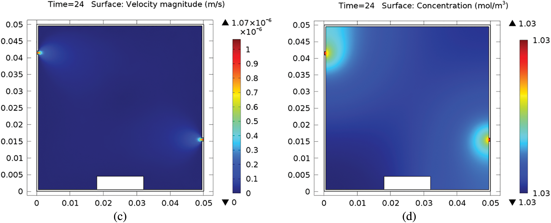
Figure 2: Effect of temperature, relative humidity profiles and wind velocity on surface condensation after 24 h

Fig. 3 represents the evolution of the maximum relative humidity inside the inverter box over all the simulation periods. The saturation threshold, where relative humidity equals 1, is reached after around 3 h, meaning that saturation occurs with a risk of condensation on the box surfaces. A Boolean saturation indicator is inserted in order to distinguish the exact saturation period. The saturation indicator is set to 1 when saturation is detected (relative humidity greater than or equal to 1) and to 0 otherwise. Fig. 4: The blue curve corresponds to the maximum relative humidity with varying moisture content and transport study, and the related condensation indicators are represented, respectively. In both models, condensation occurs after 3 h. However, when vapor diffusion is modeled as instantaneous, as in the first study, the period of time in which condensation occurs is underestimated. When the transport of diluted species interface is used to model vapor transport, a more accurate spatial representation of the vapor field is obtained. Since the vapor saturation level depends on the local values of concentration, temperature, and pressure, this improves condensation detection.

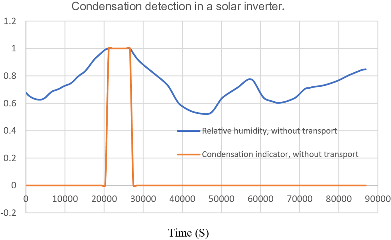
Figure 3: Maximum relative humidity over time inside the solar inverter box without transport study

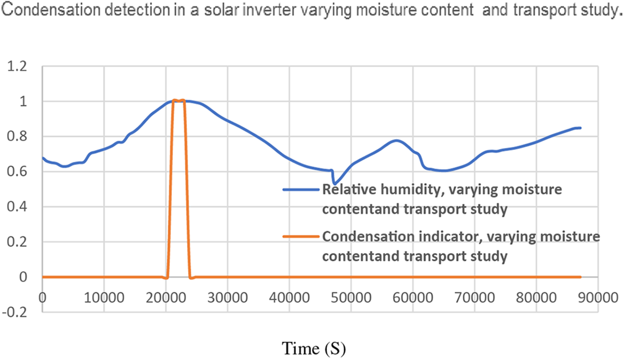
Figure 4: Condensation detection in a solar inverter varying moisture content and transport study

By using the “General Factorial Experiments” Taguchi OA method, The calculations for comparing the average reaction factors on vapor condensation for two cases (with and without varying moisture content and transport) will be determined as follows.

The effect probability, that is, the likelihood that each term’s standardized effect would be lower than the specified value, is depicted linearly in Fig. 5. By comparing the average reaction when factor “Time (A)” is high to the average response when factor “Time (A)” is low, it is possible to determine the impact of factor “Time (A)” on the response “Condensation indicator, without varying moisture content and transport study.” The major influence of a factor is the alteration in reaction brought on by a change in its level. According to the response numbers in Table 2, A′s main influence is: A = Average response at Ahigh-Average response at A lower. As a result, a plot of the reaction for the two levels of “Time′′(A)” at various levels of “Relative humidity, without varying moisture content and transport study (B)” is displayed when “A (time)” is changed from the lower level to the higher one. Assume for the moment that the response values for the two factor combinations for each were determined. Therefore, an interaction between A: time and B: relative humidity, without and with varying moisture content and transport, was studied, which exists in this case (as indicated by the non-parallel lines in Fig. 5).

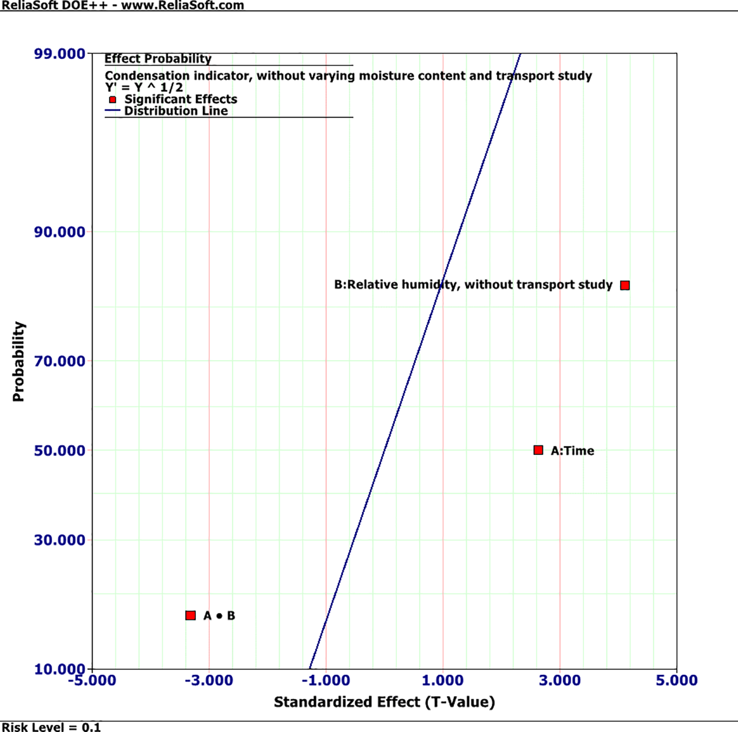
Figure 5: Optimum solution (condensation indicator) (effect of relative humidity and time) without varying moisture content and transport study

The interaction effect between and can be calculated as follows:

AB = Average response at Ahigh-Bhigh and Alow-Blow-Average response at Alow-Bhigh and Ahigh-Blow

Also, the same calculations were made with varying moisture content and transport studies. The major effect of “Time (A),” which shows that the reaction increases when the level of “Time (A)” is adjusted from low to high, would be achieved if the response at factor “Time (A)” was evaluated while holding “Relative humidity, varying moisture content, and transport study (B)” constant at its lower level. The main effect of “Time (A)” would be found, however, if the reaction at factor A was analyzed while holding B constant at its higher level, showing that the response declines when the level of Time (A) is increased from low to high, as shown in Fig. 6.

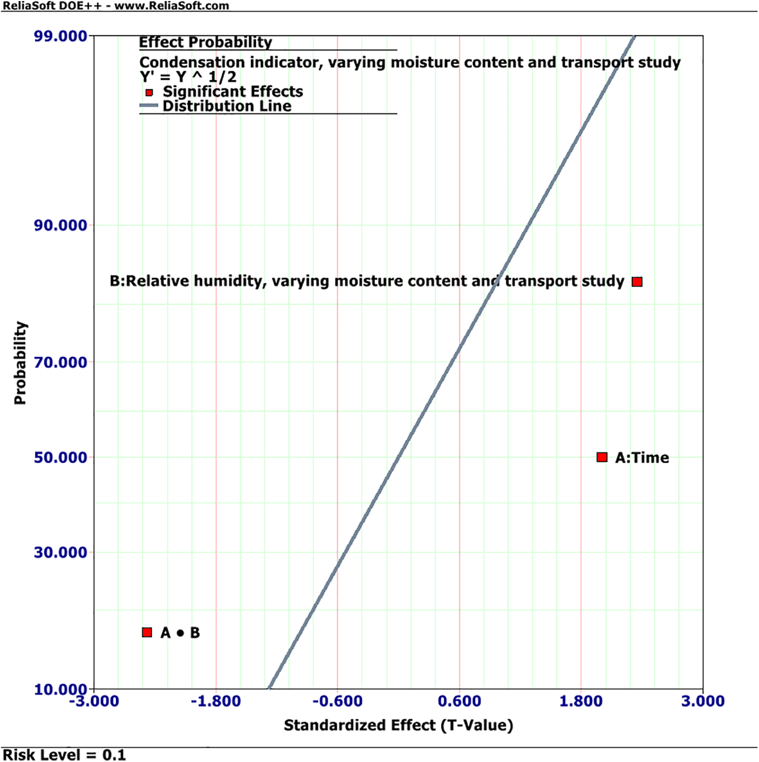
Figure 6: Optimum solution (condensation indicator) (effect of relative humidity and time) with varying moisture content and transport study

The effects of the factors (A: time and B: relative humidity) and factorial interactions between A and B on the chosen response (the condensation indicator) are summarized in Table 3 below. Both individual components and interactions, as well as groupings of factors and interactions, will be covered. The source of variation is the source that was responsible (the condensation indicator) for the variation in the measured output values. This could be an error, curvature, block, factor, or factorial interaction (A.B.). The effects will be grouped by order (principal effects, two-way interactions) if the design has more than one factor and you have chosen to utilize grouped terms in the analysis (as stated in the analysis). Sources that are highlighted in red are regarded as important and have a significant effect. The probability that there would be the same amount of fluctuation in the output if this source had no effect on it is known as the p value (also known as the alpha error or type I error). This source of variation (the condensation indicator) is deemed to have a significant impact on the result if the p value is less than alpha. The term and its p value will be shown in red in this instance. The analysis of variance (ANOVA) is included in Table 3.

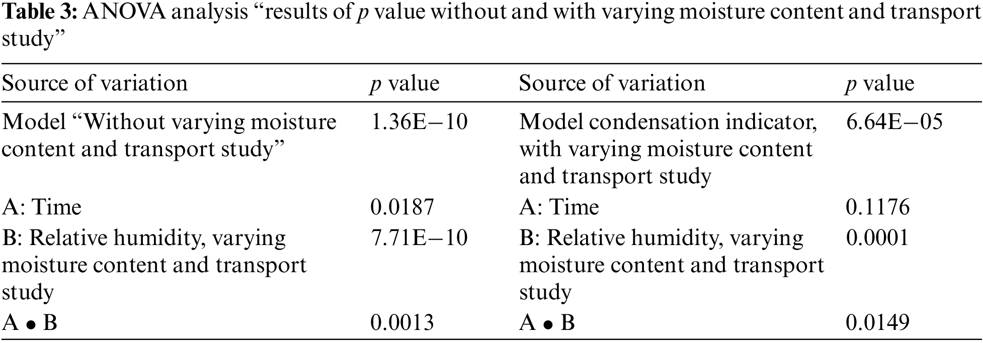
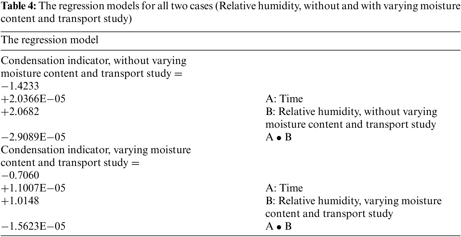
The regression coefficients for the model are −1.4233, +2.0366E−05, +2.0682, and −2.9089E−05 at (condensation indicator, without varying moisture content and transport study) and −0.7060, +1.1007E−05, +1.0148, and −1.5623E−05 at (condensation indicator, varying moisture content and transport study). In statistics, an equation created to model the relationship between dependent and independent variables is known as an estimated regression equation. The link between the regression-dependent and independent variables was originally hypothesized using either a simple or multiple regression model. Table 4 indicates the regression models for all two cases.

4  Conclusion

Photovoltaic (PV) systems are associated with a number of risks. Some photovoltaic (PV) system failures are caused by failing photovoltaic (PV) inverters. Water condensation inside the photovoltaic (PV) inverter is one of the failure reasons. The influence of external wind speed on diffusion is an effective method of moving moister air outside the inverter box. The study investigated the effects of moisture as a factor in solar inverter function failure. As interpolation functions of time T_ext (t), p_ext (t), and c_ext (t), changes in temperature, pressure, and water vapor concentration with time are computed. The numerical results of the “COMSOL Software” solution’s outcomes highlight the connection between several air velocities and reducing vapor condensation and conclude the following:

•   Calculating the movement and dispersion of moist air under the effect of wind speed allows for the identification of the problem as condensation in the PV inverter box. The device’s water vapor concentration was thought to have initially been uniform before changing in moisture content. While the movement of the interface between two diluted species is taken into account while analyzing the flow of water vapor, the effect of vapor condensation is lessened.

•   The maximum relative humidity inside the inverter box across simulated periods, which is the saturation threshold, where the relative humidity equals one, is reached after approximately 3 h, indicating that saturation has occurred with the possibility of condensation on the box surfaces. A Boolean saturation indicator was used to determine the exact saturation period. The saturation indicator was set to 1 when saturation is detected (relative humidity greater than or equal to 1) and to 0 otherwise.

•   Both models (relative humidity over time inside the solar inverter box with and without transport studies) were showing condensation after 3 h. However, when vapor diffusion is treated as instantaneous, as in the first study, the time required for condensation is overestimated. When the transport of diluted species is employed to simulate vapor transport, a more precise spatial representation of the vapor field is obtained. This increases condensation detection because the vapor saturation level is determined by the local concentration, temperature, and pressure.

Taguchi OA, according to the “General Factorial Experiments” analysis approach, has been used to compare the average response factors for vapor condensation in two instances (with and without variable moisture content and transport) as follows:

•   ANOVA analysis: “results of p value without and with varying moisture content and transport study” The effects of the factors (A: time and B: relative humidity) and factorial interactions between A and B on the chosen response (condensation indicator) are given a significant effect on all cases except “A: time” in the model condensation indicator with varying moisture content and transport study.

•   An equation is created to model the relationship between dependent and independent variables. The regression coefficients for the model are given as −1.4233, +2.0366E−05, +2.0682, and −2.9089E−05 at (condensation indicator, without varying moisture content and transport study); also, as −0.7060, +1.1007E−05, +1.0148, and −1.5623E−05 at (condensation indicator, varying moisture content and transport study).

Acknowledgement: The authors would like to express sincere gratitude to the Mechanical Engineering Department, Engineering and Renewable Energy Research Institute, National Research Centre (NRC) in Egypt for their support.

Funding Statement: This research received funding from Project Number 13040115; Code (NRC/VPRA/FSEIRPC/F05).

Author Contributions: The authors confirm contribution to the paper as follows: study conception and design: Amal El Berry, Marwa M. Ibrahim; data collection: Amal El Berry, A. A. Elfeky and Mohamed F. Nasr; analysis and interpretation of results: Amal El Berry, A. A. Elfeky and Marwa M. Ibrahim; draft manuscript preparation: Amal El Berry, Marwa M. Ibrahim. All authors reviewed the results and approved the final version of the manuscript.

Availability of Data and Materials: Data was generated by simulation.

Conflicts of Interest: The authors declare that they have no conflicts of interest to report regarding the present study.

References

1. Ismay, C., Kim, A. Y. (2019). Statistical inference via data science a ModernDive into R and the tidyverse. (1st ed.). Chapman and Hall/CRC. https://doi.org/10.1201/9780367409913. [Google Scholar] [CrossRef]

2. Tripathy, M., Joshi, H., Panda, S. K. (2017). Energy payback time and life-cycle cost analysis of building integrated photovoltaic thermal system influenced by the adverse effect of shadow. Applied Energy, 208(3), 376–389. https://doi.org/10.1016/j.apenergy.2017.10.025 [Google Scholar] [CrossRef]

3. Han, H. J., Jeon, Y. I., Lim, S. H., Kim, W. W., Chen, K. (2010). New developments in illumination, heating and cooling technologies for energy-efficient buildings. Energy, 35(6), 2647–2653. https://doi.org/10.1016/j.energy.2009.05.020 [Google Scholar] [CrossRef]

4. Tomaschitz, R. (2017). Weibull thermodynamics: Subexponential decay in the energy spectrum of cosmic-ray nuclei. Physica A, 483, 438–455. https://doi.org/10.1016/j.physa.2017.03.034 [Google Scholar] [CrossRef]

5. Vîiu, G. A. (2018). The lognormal distribution explains the remarkable pattern documented by characteristic scores and scales in scientometrics. Journal of Informetrics, 12, 401–415. https://doi.org/10.1016/j.joi.2018.02.002 [Google Scholar] [CrossRef]

6. Nie, K., Sinha, B. K., Hedayat, A. S. (2017). Hedayat Unbiased estimation of reliability function from a mixture of two exponential distributions based on a single observation. Statistics & Probability Letters, 127(2), 7–13. https://doi.org/10.1016/j.spl.2017.03.026 [Google Scholar] [CrossRef]

7. Ducrosa, F., Pamphile, P. (2018). Bayesian estimation of Weibull mixture is heavily censored data setting. Reliability Engineering & System Safety, 180, 453–462. https://doi.org/10.1016/j.ress.2018.08.008 [Google Scholar] [CrossRef]

8. Balijepalli R., Chandramohan V. P., Kirankumar K. (2017). Performance parameter evaluation, materials selection, solar radiation with energy losses, energy storage, and turbine design procedure for a pilot-scale solar updraft tower. Energy Conversion and Management, 150(2), 451–462. https://doi.org/10.1016/j.enconman.2017.08.043 [Google Scholar] [CrossRef]

9. Bazmi, A. A., Zahedi, G. (2011). Sustainable energy systems: Role of optimization modeling techniques in power generation and supply—A review. Renewable and Sustainable Energy Reviews, 15(8), 3480–3500. https://doi.org/10.1016/j.rser.2011.05.003 [Google Scholar] [CrossRef]

10. Zhu, D., Srinivasareddy, M., Paul., F. (1995). Approach for urban driving rain index by using climatological data recorded at suburban meteorological station. B&ding and Environment, 30(2), 229–236. [Google Scholar]

11. Deb C., Zhang F., Yang J., Lee S. E., Shah K. W. (2017). A review on time series forecasting techniques for building energy consumption Renewable and Sustainable. Energy Reviews, 74, 902–924. https://doi.org/10.1016/j.rser.2017.02.085 [Google Scholar] [CrossRef]

12. Zio, E. (2009). Reliability engineering: Old problems and new challenges. Reliability Engineering and System Safety, 94, 125–141. https://www.journals.elsevier.com/reliability-engineering-and-system-safety [Google Scholar]

13. Zhang, Y., Ma, S., Yang, H., Lv, J., Liu, Y. (2018). A big data-driven analytical framework for energy-intensive manufacturing industries. Journal of Cleaner Production, 197, 57–72. https://doi.org/10.1016/j.jclepro.2018.06.170 [Google Scholar] [CrossRef]

14. Vassakis, K. (2017). Big data analytics: Applications, prospects, and challenges. https://link.springer.com/chapter/10.1007%2F978-3-319-67925-9_1 [Google Scholar]

15. Garza-Ulloa, J. (2018). Chapter 5–Methods to develop mathematical models: traditional statistical analysis. In: Applied biomechatronics using mathematical models, pp. 239–371. Academic Press. [Google Scholar]

16. Sonti, V., Jain, S., Bhattacharya, S. (2016). Analysis of the modulation strategy for the minimization of the leakage current in the PV grid-connected cascaded multilevel inverter. IEEE Transactions on Power Electronics, 32(2), 1156–1169. https://doi.org/10.1109/TPEL.2016.2550206 [Google Scholar] [CrossRef]

17. Kshatri, S. S., Dhillon, J., Mishra, S. (2021). Impact of solar irradiance and ambient temperature on PV inverter reliability considering geographical locations. International Journal Heat and Technology, 39(1), 292–289. [Google Scholar]

18. Malik, A. (2022). Overview of fault detection approaches for grid connected photovoltaic inverters. E-Prime–Advances in Electrical Engineering, 2(1), 100035. https://doi.org/10.1016/j.prime.2022.100035 [Google Scholar] [CrossRef]

19. di Tommaso, A. O., Genduso, F., Miceli, R., Galluzzo, G. R. (2016). Current fault signatures of voltage source inverters in different reference frames, Capri, Italy, IEEE. pp. 599–604. https://doi.org/10.1109/SPEEDAM.2016.7525977 [Google Scholar] [CrossRef]

20. Raj, N., Mathew, J., Jagadanand, G., George, S. (2016). Open-transistor fault detection and diagnosis based on current trajectory in a two-level voltage source inverter. Procedia Technol, 25(6), 669–675. https://doi.org/10.1016/j.protcy.2016.08.159 [Google Scholar] [CrossRef]

21. Hassan, Y. B., Orabi, M., Gaafar, M. A. (2023). Failures causes analysis of grid-tie photovoltaic inverters based on faults signatures analysis (FCA-B-FSA). Solar Energy, 262(2), 111831. https://doi.org/10.1016/j.solener.2023.111831 [Google Scholar] [CrossRef]

22. Tan, Y., Liu, J., Xu, S., Zhong, P., Zhang, Q. et al. (2020). Operational reliability evaluation of PV inverter considering relative humidity and its application on power system. E3S Web of Conferences, 185, 01050. https://doi.org/10.1051/e3sconf/202018501050 [Google Scholar] [CrossRef]

23. Golnas A. (2013). PV system reliability: An operator’s perspective. IEEE Journal of Photovoltaics, 3(1), 416–421. https://doi.org/10.1109/JPHOTOV.2012.2215015 [Google Scholar] [CrossRef]

24. Li, X., Pan, C., Luo, D., Sun, Y. (2020). Series DC arc simulation of photovoltaic system based on habedank model. Energies, 13(6), 1416. https://doi.org/10.3390/en13061416 [Google Scholar] [CrossRef]

25. He, L. (2023). Chapter two–Conjugate heat transfer: Some fundamentals and recent progress. In: Abraham, J. P., Gorman, J. M., Minkowycz, W. J. (Eds.Advances in heat transfer, pp. 41–87. Elsevier. https://doi.org/10.1016/bs.aiht.2023.02.002 [Google Scholar] [CrossRef]

26. Li, G., Duan, G., Liu, X., Wang, Z. (2023). Chapter eight–Heat transfer models. In: Li, G., Duan, G., Liu, X., Wang, Z. (Eds.Moving particle semi-implicit method, pp. 143–164. Elsevier. https://doi.org/10.1016/B978-0-443-13508-8.00008-1 [Google Scholar] [CrossRef]

27. Mohr, D. L., Wilson, W. J., Freund, R. J. (2022). Chapter 9–Factorial experiments. In: Mohr, D. L., Wilson, W. J., Freund, R. J. (Eds.Statistical methods (Fourth Editionpp. 445–491. Academic Press. https://doi.org/10.1016/B978-0-12-823043-5.00009-6 [Google Scholar] [CrossRef]

28. Nelsen, T. C. (2023). Chapter fourteen–Efficient design of experiments (DOE). In: Nelsen, T. C. (Eds.Probability and statistics for cereals and grains, pp. 201–214. Woodhead Publishing. https://doi.org/10.1016/B978-0-323-91724-7.00011-3 [Google Scholar] [CrossRef]

29. Taguchi, G., Chowdhury, S., Wu, Y. (2005). Taguchi’s quality engineering handbook. Hoboken, New Jersey: John Wiley & Sons, Inc. [Google Scholar]

30. Ghenai, C., Ahmad, F. F., Rejeb, O., Hamid, A. K. (2021). Sensitivity analysis of design parameters and power gain correlations of bi-facial solar PV system using response surface methodology. Solar Energy, 223, 44–53. https://doi.org/10.1016/j.solener.2021.05.024 [Google Scholar] [CrossRef]