Numerical Predictions of Laminar Forced Convection Heat Transfer with and without Buoyancy Effects from an Isothermal Horizontal Flat Plate to Supercritical Nitrogen

Nomenclature

1  Introduction

Supercritical fluids are mainly known for their severe variation in their properties with a slight alteration in pressure and temperature. These property variations advocate the use of supercritical fluids in various aspects of the engineering realm. A detailed study by Knez et al. [1] provides a wide range of applications of supercritical fluids. Supercritical fluids have found vast applications in the processing of natural products and polymer processing over the past two decades. This is due to the lower energy consumption compared to the traditional methods. Sustainable technological solutions are the need of the hour. Hence, Supercritical fluids have also been used in chemical and biochemical reactions mainly to eliminate the use of volatile organic solvents and to reduce the consumption of raw materials. This process helps in reducing the toxic waste that is generated which is an environmentally benign solution. In recent years, Supercritical fluids have found different applications such as a refrigerant in heat pump systems and mobile air-conditioners. The exceptional heat transfer properties of supercritical fluids have been utilized in the field of energy production such as supercritical Brayton and Rankine cycles.

The literature on the issue of convective heat transport in the near-critical area reports several theoretical and experimental works. Hall et al. [2–4] provide in-depth analyses of earlier research on variable-property heat transfer and supercritical heat transfer. Pioro et al. [5] conducted a thorough analysis of the body of research on the issue of heat transmission to fluids in the near-critical region that has been published over the last fifty years. Pioro and Duffey’s review led them to the following conclusions: (i) The majority of published papers deal with the heat transfer of fluids in the near-critical region flowing inside circular tubes or channels; helium, carbon dioxide, and water are the main working fluids. (ii) The development and design of supercritical steam generators for power plants was the primary goal of these studies. A good number of analytical researches on free convection in the near-critical zone are also documented in [6–14]. Fritch et al. [6–10] have all employed the integral approach or the concept of similarity to solve their investigations’ governing equations. According to all of their predictions, the heat transfer coefficient is dependent on the respective values of Tw and T∞. The experimental values are often found to be 10% to 30% higher than the analytical predictions, with the difference increasing for greater values of ΔT, even when there is qualitative agreement between their analytical predictions and experimental values. Each of these studies is conducted for ΔT < 16 K. To account for the variation of all fluid properties in the near-critical region, Seetharam et al. [11–14] modified the Patankar–Spalding numerical scheme and numerically solved the governing equations of the boundary layer for free convection from a vertical surface. They have also found solutions for high ΔT values (up to 30 K) and suggested correlations to figure out the heat transfer coefficients. The topic of forced and mixed convection from a flat plate to fluids in the near-critical zone has been the subject of very few experimental investigations [15,16] that have been published in the literature. The temperature and boundary layer velocity profiles for a turbulent forced flow of near-critical nitrogen past a vertical flat plate have been observed by Simoneau [15]. Their measurements were compared under identical operating conditions, except for the boundary layer being at a temperature lower than the critical temperature. The comparison revealed a maximum difference between the wall and the free stream at the near-critical velocity profiles, which are significantly different from each other. The near-critical profile exhibited a significantly higher Grashoff number, indicating the presence of a strong body force effect. Additionally, they noticed that even at high Reynolds numbers, body forces seem to be exaggerated when close to the critical point. Experiments on forced convection heat transfer from near-critical nitrogen flowing over a horizontal flat plate were carried out by Graham et al. [16]. The heated surface has an upward and downward orientation. He made a comparison between the outcomes and past research [15]. The thermodynamic critical temperature was not always reached by the boundary layer temperatures.

It was observed that varying the velocity and temperature profiles in the three directions does not significantly change when the wall temperature is lower than the thermodynamic critical temperature. When the flow enters the critical temperature area, the heat transfer coefficient decreases, the velocity and temperature profiles smooth down, and this phenomenon happens across all three dimensions. In an upward flow, the velocity between the wall and the free stream was the highest. A noticeable deviation of the velocity profiles was evident in horizontal flow when the heated surface was directed upward. Stagnant zones with near-zero velocities exist in horizontal flows with the heated surface directed downward. Results from all of their experiments indicate the flat plate’s turbulent area, where Rex > 9.3 × 105. Fluids flowing past a flat plate in the near-critical zone have received surprisingly little attention from analytical studies addressing the issue of laminar-driven and mixed convection heat transfer.

Recently, Sri Sathya Sai et al. [17] have numerically investigated the problem of turbulent flow over an isothermally heated horizontal flat plate using supercritical nitrogen. The authors have used the k−ε Realizable model with enhanced wall treatment to solve the heat transfer problem in the forced and free convection regime. The authors have proposed a Nusselt number correlation for each regime incorporating the effects of buoyancy forces. The authors have concluded by noting considerable deviations in the velocity and temperature profiles due to property variations when compared to constant property cases. The correlations proposed hold good for a P∞/Pcr range of 1.1 to 1.4 and a Reynolds number range of 105 to 108.

Hardly any information is available in the literature on the problem of laminar forced convection with and without buoyancy effects for heat transfer from a horizontal isothermal flat plate to supercritical fluids. The objective of the present investigation is to numerically solve the governing equations for the laminar forced flow of supercritical Nitrogen over a horizontal isothermal flat plate with a heated surface facing downwards. The flow with and without buoyancy effects is studied and based on the numerical predictions, correlations to evaluate the local Nusselt number are proposed.

2  Property Variations in Supercritical Fluids

The heat transfer behavior using supercritical fluids can be accurately predicted by including the variations in the thermo-physical properties in the investigation. Figs. 1 to 3 represent the variation of different thermo-physical properties with temperature at a pressure of 37.35 bar (P∞/Pcr−1.1) [18]. It can be seen from Fig. 1, that CP starts from a lower value, reaches a maximum value, and then the trend tends to decrease again. The state point where the maximum value of Cp occurs is called the pseudo-critical point and the temperature at this state point is known as pseudo-critical temperature T∗. While in Figs. 2 and 3, it can be observed that near T∗, the values of k,μ & ρ reduce by factors of 3 to 6, whereas Cp,i & β increase by huge factors of 8 to 14. A general trend that can be observed in all three figures is that there is an anomaly in all the thermo-physical properties close to the near-critical region.

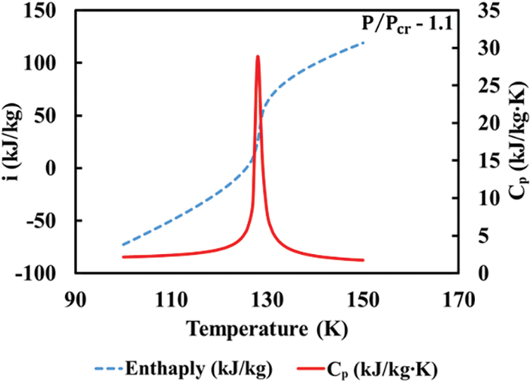
Figure 1: Variation of specific heat at constant pressure and enthalpy with temperature for nitrogen at 37.35 bar

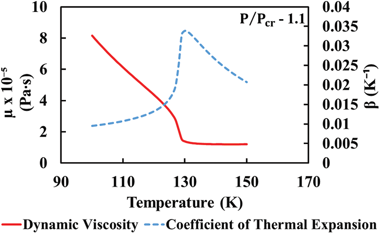
Figure 2: Variation of dynamic viscosity and coefficient of thermal expansion with temperature for nitrogen at 37.35 bar

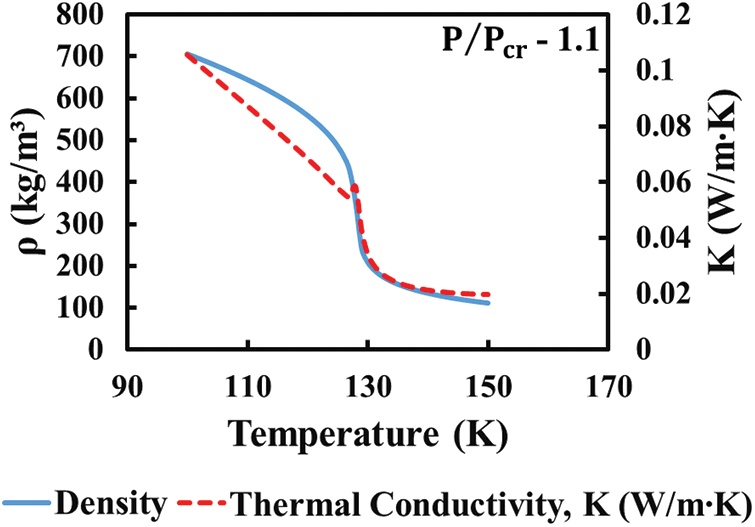
Figure 3: Variation of thermal conductivity and density with temperature for nitrogen at 37.35 bar

3  Validation

Fig. 4 depicts the variation of CP with temperature for different values of P∞/Pcr ranging from 1.1 to 1.4. It can be clearly distinguished that for pressures close to the critical pressure, CP varies severely (by a factor of 15 for P∞/Pcr value of 1.1) with temperature but whereas for pressures that lie away from the critical point (P∞/Pcr − 1.4), this drastic change in CP with temperature is not observed (the change is reduced to a factor of about 3 for a P∞/Pcr value of 1.4). The work conducted by Ingrid Martorell et al. [19] deals with the heat transfer from a horizontal flat plate heated upwards. Several plate dimensions have been used in this work based on the aspect ratios. The range of aspect ratio considered in this work is 0.036 to 0.43 where the aspect ratio is defined as the ratio between the width of the plate to the length of the plate. Experiments have been conducted for various values of Rayleigh numbers which range from 290−3.3×105. This work finds various applications in the design of printed circuit boards which are predominantly used in the automotive industry. The plates used in this work are made of copper and stainless steel. Calculations have been performed to predict the transverse profiles of the heat flux and surface temperature and to picture the structure of the flow. The copper plate has a thickness of 35 µm whereas the stainless-steel plate has a thickness of 50 µm. As the top surface of the plate is maintained at isothermal conditions, the bottom surface of the plate is insulated by a fiberglass layer of 3 cm thickness. The plate is placed in a rectangular Plexiglas enclosure with dimensions 84 cm × 70 cm × 50 cm. The working fluid used in this work is air at 1 atmospheric pressure. A K-type thermocouple was used to measure the temperatures. The temperature difference range used in this work lies between 3≤ΔT≤20 K. Results obtained for a very low value of ∆T are not satisfactory due to uncertainties in measurement using the thermocouple. Also, when the plate is at a higher value of ΔT, it is not possible to maintain the longitudinal exothermicity. The authors of this work have performed numerous experimental studies by varying the aspect ratios and the Rayleigh number which leads to the following equation:

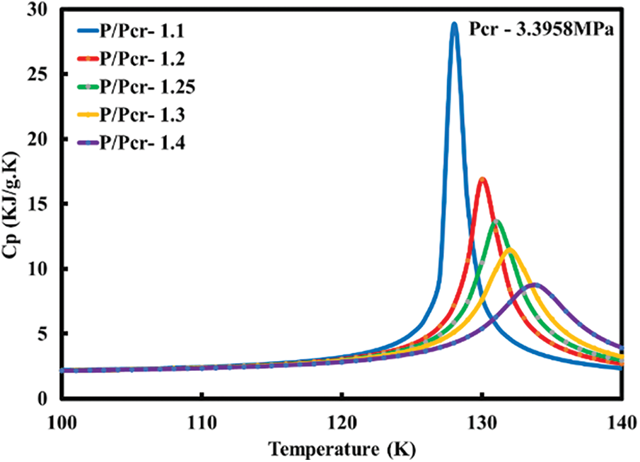
Figure 4: Variation of Cp with temperature for nitrogen at different ratios of P∞/Pcr

Nuw=1.23Raw0.173(1)

The authors concluded that the present experiments showed that there is no significant dependence on the Nusselt number on the dimensions of the plate. Using this work as the datum, validation has been performed by incorporating the finite volume method using the commercial software “ANSYS Fluent 19.2”. In the present validation, a copper plate with an aspect ratio of 0.109 has been used with a plate length of 23 cm and a plate width of 2.5 cm. The free stream velocity is set to 0.653 m/s. Different values of ambient and wall temperatures have been used to satisfy the range of the temperature difference mentioned in [19]. The laminar model with viscous effects has been used for the validation. The solution method incorporated in the solver is coupled with second-order pressure for better accuracy. The pseudo-transient flow was enabled to get fast and reliable convergence. The scaled residuals were set to a value of ≤10−5 for the energy and momentum equations and ≤10−6 for the continuity equation. Fig. 5 shows the comparison between the experimental data from the correlation as given by Martorell et al. [19], data points given by Corcione [20], and the computational values obtained from Fluent. It is observed that the maximum deviation obtained in these computational case studies is less than ±7% when compared to the Nusselt number correlation as given by Eq. (1). The same values were also compared with the article by Corcione [20] and the deviations were found to be less than ±6%. Therefore, a 3D validation of heat transfer over a horizontal flat plate is in good agreement with the 2D discretization and the experimental data available in the open literature.

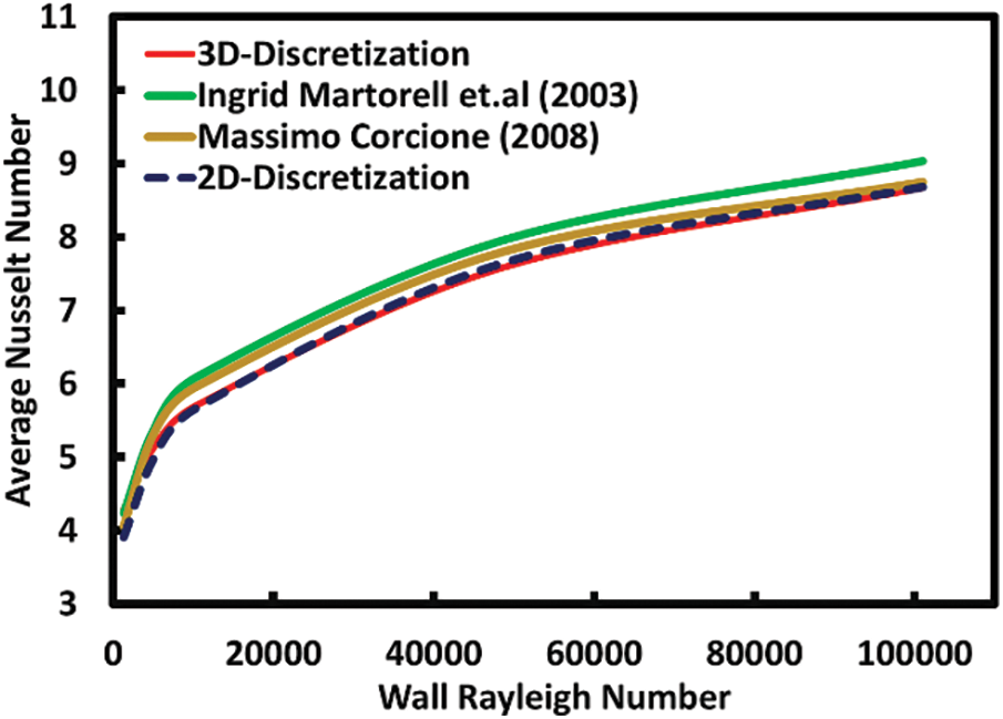
Figure 5: Comparison of experimental and numerical Nusselt numbers with wall Rayleigh number

4  Methodology

4.1 Flow Domain

In Section 3, a brief validation is described by using both the 3-dimensional discretization and the 2-dimensional discretization. Computations were performed using both methods and were compared to the available experimental and numerical solutions. It can be noted from Fig. 5 that there is a very minimal deviation between the 3D and 2D discretization. Hence, with reduced computational time and reasonably accurate results, the 2D discretization method has been implemented in this current work. The flow is assumed to be two-dimensional and steady. The dimensions of the plate are as follows: the length of the plate is 23 cm in the direction of the flow and 2.5 cm normal to the flow direction. It can be noted from Fig. 6 that a pre-stabilization length of 5 cm has been given to the geometry to obtain a fully developed laminar flow without any reverse flow or vortex generation at the entry length of the plate. Two regimes of heat transfer have been studied in the present investigation. The regimes are forced convection with buoyancy effects and forced convection with negligible buoyancy effects. The heat transfer characteristics have been evaluated over a range of five different ratios of P∞/Pcr starting from a value of 1.1 till 1.5, where the critical pressure (Pcr) of nitrogen is 3.396MPa. Five different wall temperatures were chosen in such a fashion that two of the values were below T∗, one equal to T∗ and two other greater than T∗ with three different values of free stream velocity. These parameters were used in varying combinations to obtain a large data set to predict the heat transfer progression in the supercritical region with utmost accuracy. Specifying appropriate boundary conditions for the flow field is of prime importance to simulate the required case accurately. A velocity inlet boundary condition is applied at the inlet where three different values of free stream velocities were quantified–1.4, 1.6, and 1.8 m/s for the case of forced convection without buoyancy effects and 0.25, 0.3, and 0.35 m/s for the case of forced convection with buoyancy effects. An ambient temperature (T∞) of 110 K was maintained throughout all the case studies. A no-slip boundary condition was specified at the wall which was maintained at an isothermal condition. The region opposite the isothermal wall is specified as a symmetry boundary condition that acts as a far-field. It is of prime importance to stipulate the acceleration due to gravity in the negative y-direction to capture the boundary layer effects with buoyancy forces. Since supercritical fluids have varying properties with temperature, the default ideal gas property values cannot be used in this scenario. Hence, the piece-wise linear option available in the commercial software ANSYS Fluent 19.2 was used to input different values of k,μ,ρ and Cp at different temperatures which were obtained from NIST [21] in such a way that the properties encapsulate the range of the present problem.

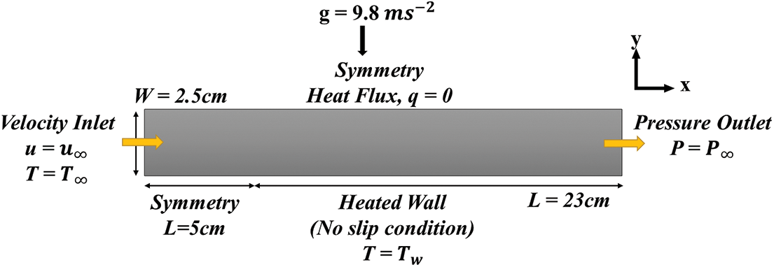
Figure 6: Appropriate boundary conditions in the 2D flow domain

4.2 Numerical Method

An important factor while examining convection heat transfer is the identification of the type of boundary layer, i.e., laminar, or turbulent. Convection transfer rates strongly depend on this factor. The current work completely concentrates on the laminar boundary layer. In a laminar boundary layer, streamlines are highly distinguishable and ordered along the direction of fluid flow. A triggering mechanism is a major cause of the transition from the laminar to the turbulent regime. These triggering mechanisms can be unsteady flow structures, disturbances within the boundary layer, and fluctuations in the free stream. A non-dimensional, definitive way to predict the nature of the boundary layer by using the Reynolds number (Rex<Rex,crfor laminar flows). Where, Rex,cr is the critical Reynolds number. For flows flowing over a flat plate, the critical Reynolds number can vary from 5×105−3×106 depending on the turbulence level of the free stream and the surface roughness [22]. In the present study, an investigation for forced convection heat transfer with laminar flow is examined in detail. To calculate the heat transfer parameters, certain equations have been used by the solver to provide accurate and reliable results. The three most important equations while solving such problems are the continuity, momentum, and energy equations. These three equations constitute and account for the heat transfer using fluids. The continuity equation for the case of a steady laminar incompressible flow without free-surface effects is commonly given by Eq. (2). Most of the solvers make use of the continuity equation derived from the Navier-Stokes equation as shown by Eq. (3) [23].

∇→⋅V→=0(2)

(V→⋅∇→)V→=−1ρ∇→P′+ν∇2V→(3)

Eq. (2) is commonly known as the conservation equation whereas Eq. (3) is known as the transport equation which denotes the transport of the linear momentum throughout the computational domain [23]. The modified form of pressure (P′) is used in these equations due to the absence of free-surface effects. The more advanced form of the momentum and continuity equations used by solvers are represented by the following equations:

∂u∂x+∂v∂y+∂w∂z=0(4)

The general momentum equation in three flow directions, that is x, y and z are as follows:

u∂u∂x+v∂v∂y+w∂w∂z=−1ρ∂P′∂x+ν(∂2u∂x2+∂2u∂y2+∂2u∂z2)(5)

u∂u∂x+v∂v∂y+w∂w∂z=−1ρ∂P′∂y+ν(∂2v∂x2+∂2v∂y2+∂2v∂z2)(6)

u∂u∂x+v∂v∂y+w∂w∂z=−1ρ∂P′∂z+ν(∂2w∂x2+∂2w∂y2+∂2w∂z2)(7)

The following equations are strictly applicable to incompressible flows. These equations must be modified in order for them to be applicable for steady laminar compressible flows. Eqs. (8)–(12) [24] represent the continuity, momentum, and energy equations for compressible flows.

∂(ρu)∂x+∂(ρv)∂y+∂(ρw)∂z=0(8)

Similarly, the momentum equations are compiled over three flow directions namely x, y, and z.

ρ(u∂u∂x+v∂u∂y+w∂u∂z)=ρgx−∂P∂x+∂∂x(2μ∂u∂x+λ∇→⋅V→)+∂∂y(μ(∂u∂x+∂v∂x))+∂∂z(μ(∂w∂x+∂u∂z))(9)

ρ(u∂v∂x+v∂v∂y+w∂v∂z)=ρgy−∂P∂y+∂∂y(2μ∂v∂y+λ∇→⋅V→)+∂∂x(μ(∂v∂x+∂u∂y))+∂∂z(μ(∂v∂z+∂w∂y))(10)

ρ(u∂w∂x+v∂w∂y+w∂w∂z)=ρgz−∂P∂z+∂∂z(2μ∂w∂z+λ∇→⋅V→)+∂∂x(μ(∂w∂x+∂u∂z))+∂∂y(μ(∂v∂z+∂w∂y))(11)

An important equation while solving any heat transfer-fluid flow problem is the energy transport equation. The energy equation for a compressible laminar flow is given by equation.

ρCp(u∂T∂x+v∂T∂y+w∂T∂z)=βT(u∂P∂x+v∂P∂y+w∂P∂z)+∇→⋅(k∇→T)+Φ(12)

The above partial differential equations (Eqs. (9) to (12)) are converted to algebraic equations by the solver’s inbuilt algorithm which computes the required fluid flow and heat transfer parameters. The present investigation incorporates the pressure-based solver which is commonly used to compute characteristics of incompressible flows and slightly compressible flows. Since supercritical fluids portray a trait of varying properties with temperature and pressure, it has been sure that these property variations have been considered by incorporating fifty data points for the independent properties using the piecewise linear option offered by ANSYS Fluent 19.2 [25]. The partial differential equations are solved sequentially by the pressure-based solver which takes the property values at each iteration [25].

Using these models without enabling certain options would not yield the correct results. Hence, the laminar model with viscous effects has been used in this study to actively capture the boundary layer effects. In addition to this, a no-slip boundary condition is specified at the velocity boundary layer and a second-order differential scheme is used to calculate the gradients [26]. Most of the liquid flows can be considered as incompressible. But for gaseous flows, it is important to estimate the Mach number to ascertain it as an incompressible flow [23]. Hence, the Mach numbers have also been calculated to prove the usability of the pressure-based solver as shown in Table 1.

For a flow to be considered incompressible, the Mach number should be less than 0.3 [27]. This assumption is rational at low values of Mach numbers which holds good for the present investigation. It can be observed from Table 1 that for both minimum (0.25 m/s) and maximum (1.8 m/s) values of the velocity, the Mach numbers are significantly less than 0.3 which advocates the use of the pressure-based model for this investigation.

The finite volume method has been used in this study to evaluate the algebraic equations obtained from the partial differential equations computed by the differencing scheme. The coupled algorithm has been used for the computational study. The coupled scheme results in an efficient and robust single-phase implementation of steady flows when compared to the default SIMPLE-type pressure-velocity coupling. This coupled algorithm solves the pressure and momentum-based continuity equations together to reduce the computational time. A second-order upwind scheme was set to discretize the pressure, momentum, and energy equations. A Least Squares Cell-Based approach was used for the gradient spatial discretization. A pseudo-transient analysis was performed to obtain faster and more efficient results. A pseudo-transient approach is a form of implicit under-relaxation for steady-state cases [24].

The pseudo transient explicit under-relaxation factors were set to 0.5 for momentum, pressure, and density, 1 for body forces, and 0.75 for energy for attaining solution stabilization. The scaled residuals were to be set to 10−6 from a default value of 10−3 for solving continuity, x, y momentum and the energy equation. Computations performed with individual values of 10−6 and above are known as tightly converged solutions. This in turn indicates that the solution is well normalized and has converged within the required range [24].

4.3 Grid Independence Study

Grid independence study plays a vital role in any computational analysis. The purpose of a mesh independence study is to obtain results that do not fluctuate with the element size. This ensures that the solution obtained is uniform throughout with minimal deviation. The geometry in the present study was discretized using the face mesh option along with the inflation layer near the heated surface. Inflation layers are added near the heated surface to capture the slightest variations in the boundary layer. A uniform set of quadrilateral elements has been used to mesh the face of the plate. The quality of the generated mesh was based on the following parameters: skewness, orthogonal quality, and element quality. It is often ascertained as a good practice to keep the average and maximum value of skewness to be less than 0.4 and 0.9, respectively. Similarly, the average and minimum values of both orthogonal and element quality are greater than 0.7 and 0.1, respectively. With drastic property changes and distortions close to the pseudo-critical point with the use of supercritical fluids, it is of prime importance to have a geometry with an appropriate mesh topology as it plays a deterministic role in the heat transfer rates in the flow. Grid independence was achieved by varying the size of each element. The investigation is performed by changing the number of mesh elements from a value of 35,000 to a value of 738,000. Table 2 showcases the various mesh elements used in this study and the corresponding outlet temperatures and heat transfer coefficient values.

The variation of outlet temperature and the heat transfer coefficient is plotted against the mesh density as displayed in Fig. 7. After an element size of 200,000, it can be noted from the above figure that mesh independence is achieved. Therefore, an element size of 345,000 has been used for the rest of the case studies. This has been selected based on the following criteria: grid independence, reduced computational time, and significantly accurate data.

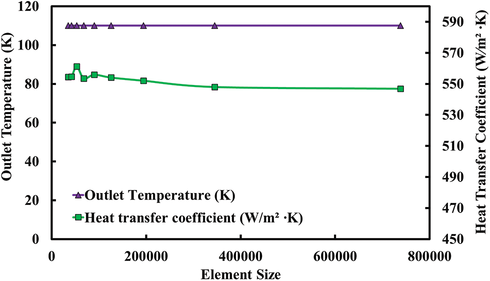
Figure 7: Grid independence study for a particular case

5  Results and Discussions

Computations for laminar, forced convective heat transfer were performed for a total of 1080 data points by varying the following parameters namely, operating pressure, wall temperature, and free stream velocity which include 540 data points for forced convection with buoyancy effects and 540 data points for forced convection without buoyancy effects.

This sample space was categorized into two major regimes based on the value of (GrxRex2). If the fraction, GrxRex2<0.1, it is said to be in the forced convection regime without any significant buoyancy effects. If it lies in the range of 0.1<GrxRex2<10, it is known to be in the forced convection regime with significant buoyancy effects.

The surface heat flux (q) at different points along the plate is determined using the post-processing section available in the ‘ANSYS Fluent 19.2’. The various locations along which the heat transfer characteristics are determined are as follows, x = 0.0025, 0.007, 0.0115, 0.016, 0.0205, and 0.025 m. These points were chosen based on the concept of the transition boundary layer. The value of x at 0.025 m is the location up to which the flow remains laminar. This means that whenever the value of x exceeds 0.025 m, the flow transfers to a pre-turbulent regime which involves the concept of transition boundary layer. Using the values of heat flux at these salient points, the values of the heat transfer coefficient and Nusselt numbers are calculated. The temperature and velocity profiles have also been discussed in detail in the upcoming sub-sections.

5.1 Velocity Profiles

Fig. 8 shows the velocity profile for the case of forced convection without significant buoyancy effects for three values of (Tw−115K(Tw<T∗), Tw−128.24K(Tw=T∗) and Tw−140K(Tw>T∗). It can be seen from these profiles that as Tw increases, the velocity profile becomes flatter thereby increasing the velocity gradient at the wall, which in turn increases the wall-shear stress and the drag coefficient. However, the velocity profiles for the case of forced convection with buoyancy effects, shown in Fig. 9 specify that for the case when Tw−115K(Tw<T∗), i.e., when T∗ lies outside the boundary layer, the velocity profile is smooth, whereas for the other two cases, namely for Tw=T∗ and Tw>T∗, there is distortion in the velocity profile and this distortion occurs at the location where the fluid temperature is in the neighborhood of T∗. This distortion of the velocity profile near T* can be attributed to the fact that for fluid temperature less than T*, Cp increases with temperature reaches a maximum at T* and then decreases with an increase in fluid temperature. A similar trend is observed for the fluid property β which affects the buoyancy force distorting the velocity profiles as well as the temperature at the location where the fluid temperature is close to T*. This distortion affects the velocity gradient at the wall which affects the wall shear stress. How much the velocity gradient is affected depends on how close the location of T∗ is concerning the heated wall. It can be observed from Fig. 9, that for the case when Tw>T∗, the distortion has considerably reduced the velocity gradient at the wall thereby decreasing the wall shear stress. Thus whenever T∗ lies within the boundary layer, the buoyancy forces play a major role in deciding the wall shear stress.

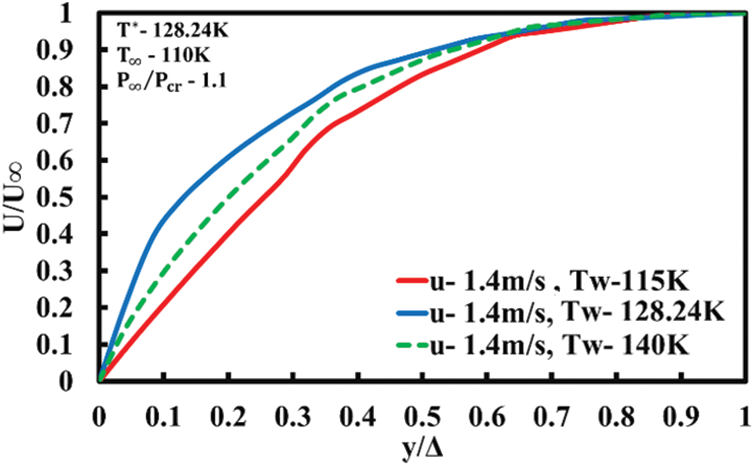
Figure 8: Velocity profile for forced convection without buoyancy effects (P∞ = 37.35 bar)

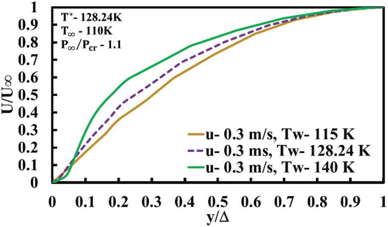
Figure 9: Velocity profile for forced convection with buoyancy effects (P∞ = 37.35 bar)

5.2 Temperature Profile

Temperature profiles for the cases without buoyancy effects are shown in Fig. 10 for three values of wall temperatures, Tw−115 K(Tw<T∗), Tw−128.24 K(Tw=T∗) and Tw−140 K(Tw>T∗). It can be noted from these profiles that as Tw increases the temperature profile becomes flatter thereby increasing the temperature gradient at the wall, which successively increases the heat transfer coefficient and hence the Nusselt number. Also, distortions are not observed in the temperature profile, even when T∗ lies within the boundary layer because the buoyancy forces are negligible to affect the temperature profiles. However, the temperature profiles for the cases of forced convection where buoyancy forces play a vital role, as shown in Fig. 11 indicate that for the case when Tw−115 K(Tw<T∗), i.e., when T∗ lies outside the boundary layer, the temperature profile is smooth without any distortions, but whereas for the other two cases, namely for Tw=T∗ and Tw>T∗, there are distortions in the temperature profiles and this distortion occurs at the location where the fluid temperature is in the neighborhood of T∗. The reason for these distortions of the temperature profiles is the same as those mentioned under the section “velocity profiles”. This distortion will in turn affect the temperature gradient (decreases the temperature gradient) at the wall which sequentially decreases the heat transfer coefficient. The dependency on the location of T∗ concerning the wall accounts for the extent to which the temperature gradient at the wall is affected. Fig. 11 also indicates, that for the case when Tw>T∗, the distortion has considerably reduced the temperature gradient at the wall thereby decreasing the heat transfer coefficient. Thus whenever T∗ lies within the boundary layer, the buoyancy forces play a substantial role in deciding the wall shear stress as well as the heat transfer coefficient. The distortion of both the temperature and velocity profiles due to the location of T∗ within the boundary layer can be attributed to the change in the sign of the slope of dCpdT across T∗.

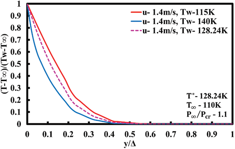
Figure 10: Temperature profile for forced convection without buoyancy effects (P∞ = 37.35 bar)

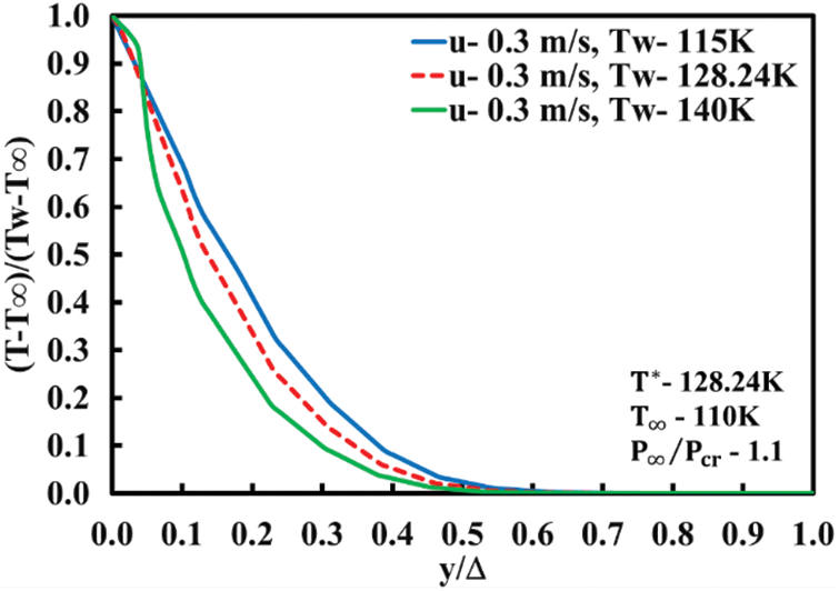
Figure 11: Temperature profile for forced convection with buoyancy effects (P∞ = 37.35 bar)

5.3 Variation of Other Heat Transfer Parameters

5.3.1 Variation of Heat Transfer Coefficient and Nusselt Number along the Length of the Plate

The variation of Nusselt number with x is shown in Fig. 12 for forced convection without buoyancy effects for three cases of Tw, namely, Tw−115 K(Tw<T∗), Tw−128.24 K(Tw=T∗) and Tw−140 K(Tw>T∗).

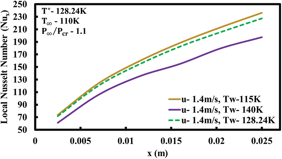
Figure 12: Variation of Nusselt number along the plate length for forced convection without buoyancy effects (P∞ = 37.35 bar)

It can be observed that as the value of x increases, the Nusselt number increases as well. This holds for all three cases and decreases as Tw approaches T∗. An analogous trend is also observed for the case where buoyancy forces are dominant as shown in Fig. 13. It can also be observed at a given location (x) for the same wall temperature, the Nusselt number for the case of forced convection without buoyancy effects is higher than that for forced convection with buoyancy effects thereby highlighting the effect of buoyancy forces on Nusselt number. It can be noted from Fig. 12 that the curves for all values of ΔT are smooth with very minimal distortions. It can be ascertained that buoyancy effects do not affect the local Nusselt number for small values of ΔT. But buoyancy forces do affect the Nusselt number when the temperature differences are very high. The difference in the minimum and maximum values of the local Nusselt number is prominent when both plots are compared. For instance, the minimum value for forced convection with significant buoyancy force is approximately 25 and for the case of without buoyancy effects, the value turns out to be 55 when the wall temperature is 140 K. Similarly, the maximum value for the case with buoyancy effects is around 95 and for without buoyancy effects is 230 when the wall temperature is 115 K. In conclusion, it can be said that for the case when Tw<T∗, it leads to the maximum value of Nusselt number whereas the case when Tw>T∗ leads to the minimum values of the Nusselt number.

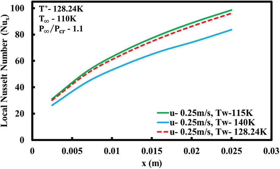
Figure 13: Variation of Nusselt number along the plate length for forced convection with buoyancy effects (P∞ = 37.35 bar)

A comparison between the predicted Nusselt numbers with constant property solutions is shown in Figs. 14 and 15. It can be noted from Fig. 15 that for values of Tw below the pseudo-critical temperature, T∗ the proposed prediction is in good agreement with the constant property solutions with very minimal deviations (less than 2%). When the value of Tw lies nearby of T∗ and is increased to T∗, the deviations increase significantly (10%–75%). The maximum deviation is found to be at a wall temperature of 140 K which lies far away from T∗. This can be attributed to the influence of buoyancy forces on the heat transfer coefficient. From Fig. 14, it can be observed that as Tw approaches T∗, the proposed correlations deviate considerably from the constant property solution. But whereas, as Tw moves away from the critical temperature, T∗, the deviation between the proposed predictions and constant property solution is considerably minimized. This nature of the curves can be ascribed to the severe deviations in the thermo-physical properties of supercritical fluids which have been accounted for in the present predictions.

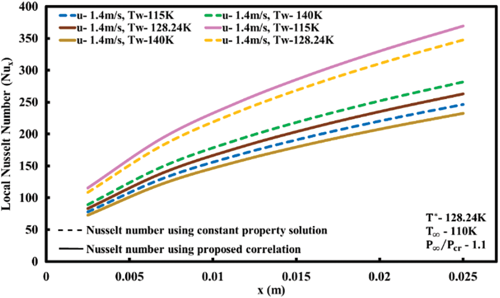
Figure 14: Variation of Nusselt number along the plate length using constant property solution and proposed correlation for forced convection without buoyancy effects (P∞ = 37.35 bar)

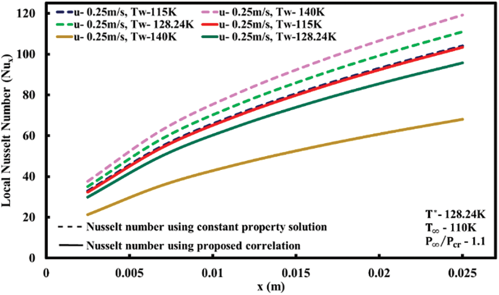
Figure 15: Variation of Nusselt number along the plate length using constant property solution and proposed correlation for forced convection with buoyancy effects (P∞ = 37.35 bar)

Fig. 16 represents the variation of heat transfer coefficient with ΔT ranging from 5 to 30 K at a distance of 0.0025 m from the leading edge of the plate. The values of ΔT were chosen in such a way that two values of wall temperature are less than T∗, one is equal to T∗ and two values are greater than T∗. For both the heat transfer regimes, the heat transfer coefficient reduces, reaches a maximum value, and then further reduces to a lower value. The heat transfer coefficient is found to depend not only on the temperature difference but also on the distinct values of Tw and T∞. It can be evidently observed that the heat transfer coefficients are significantly higher for forced convection without buoyancy forces. For ΔT values which lie near T∗, distortions in the form of a peak are observed in both regimes.

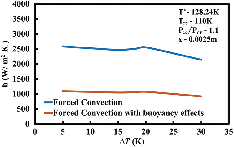
Figure 16: Distribution of heat transfer coefficient with ΔT at x = 0.0025 m (P∞ = 37.35 bar)

5.3.2 Variation of Wall Shear Stress

Figs. 17 and 18 depict the variation of the wall shear stress along the length of the plate. A general decreasing trend is observed for both the heat transfer regimes (convection with and without buoyancy effects) with an increasing value of x. The rate of this decrease is higher for the case of forced convection with buoyancy effects when equated to its counterpart. It can be noted from both plots that the curve undergoes a rapid depression and then flats out over the trailing edge of the plate. The temperature difference plays an ardent role in the trends of the above plots. The maximum value of the wall shear stress can be observed to occur near the leading edge of the plate where the flow starts to develop. In general, the value of wall shear stress is significantly higher for the case of forced convection heat transfer without buoyancy effects when compared to the case where the buoyancy effects play a key role. For lower values of ΔT, where Tw is less than T∗, that is if T∗ lies outside the boundary layer, the predicted wall shear stress values match the constant property solution with minimal deviations. Whereas, as ΔT is increased to larger values such as 30 K, the predicted values deviate significantly from the constant property solution. This clearly shows the effect of buoyancy forces on wall-shear stress. At a value of x = 0.007 m, a sudden dip of the wall shear stress can be observed vividly for both the heat transfer regimes. This abnormality is severe for wall temperatures equal to or greater than the critical temperature.

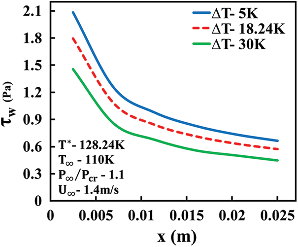
Figure 17: Wall shear stress distribution along the plate length for forced convection without buoyancy effects for P∞ = 37.35 bar

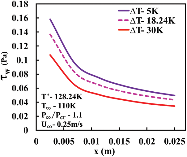
Figure 18: Wall shear stress distribution along the plate length for forced convection with buoyancy effects (P∞ − 37.354 bar)

6  Nusselt Number Correlations

6.1 Correlations for Laminar Forced Convection without Buoyancy Effects

Seven formats of correlations which are available in the literature for supercritical fluids are used to compare the predicted Nusselt numbers with the actual numerical predictions. All seven formats consider the variation of the fluid properties in the correlation in one way or the other. These formats are as follows:

(i) Format F1: This format for forced convection without buoyancy effects [GrxRex2<0.1] considers the variation of fluid properties by introducing four property rations in the correlation and the correlation is given by

(Nux)fcF1=a(Rexb)(Pr)c(C¯pCp\infty )d(ρ∞ρw)e(µ∞µw)f(k∞kw)g(13)

Gustavo et al. [26] have shown that the above format gives better agreement with the actual predictions based on their comparison of available data with the various forms of correlations. In the present investigation, based on Nux at 540 data points and using multiple linear regression analysis, Eq. (13), takes the following form:

(Nux)fcF1=0.398×(Rex0.505)(Pr∞)−0.144(C¯pCp\infty )0.101(ρ∞ρw)−0.015(µ∞µw)−0.0136(k∞kw)−0.1274(14)

The R2 value concerning Eq. (14) is found to be 0.9986. Out of 540 data points, 536 data points (99.26%) have deviations less than 5% [% deviation = ((Nux) by correlation/(Nux) by numerical prediction) – 1) 100] and the remaining 4 data points have deviations between 5% and 9%.

(ii) Format F2: In this format, the correlation for Nux has only two property ratios, namely, the specific heat ratio (C¯pCp∞) and the density ratio (ρ∞ρw). This format assumes that the nature of variation of viscosity and thermal conductivity are similar to the variations of density and specific heat for supercritical fluids and hence the specific heat ratio and the density ratio will also account for the variation of viscosity and thermal conductivity. The multiple linear regression analysis for this format yields the following correlation:

(Nux)fcF1=0.314×(Rex0.505)(Pr∞)0.277(C¯pCp\infty )0.148(ρ∞ρw)−0.159(15)

The R2 value for this correlation is found to be 0.998. The deviation is less than 5% for 538 data points (99.6%) out of 540 points and the remaining two points have deviations between 5 and 8 percent.

(iii) Format F3: This method has been proposed by Ghajar et al. [28] for free convective heat transfer from vertical isothermal flat plates to supercritical fluids. In this method, a characteristic temperature, called ‘reference temperature’, Tref is chosen at which the properties appearing in the nondimensional groups (Nu, Gr, Pr, etc.) are evaluated. The constant property results at that temperature are then used to evaluate the Nusselt number for supercritical fluids. Typically, this temperature may be the surface temperature Tw, the bulk fluid temperature T∞, or a temperature in between Tw and T∞. Based on this concept, Tref is expressed as follows:

Tref=Tw–r[Tw−T∞](16)

In the investigations (experimental/analytical) reported in the literature for reference temperature, the parameter ‘r’ of Eq. (16) has been assumed to have a constant value. This assumption is valid only when the thermodynamic and transport properties of the fluid under consideration do not vary significantly within the boundary layer. For such cases determination of the reference temperature constant, r is simple and straightforward. But in the case of heat transfer in supercritical fluids, this assumption is not valid as the thermos physical properties of the fluid vary very severely, especially when the fluid pressure is near to the critical pressure and the temperatures Tw and T∞ are close to the pseudo-critical temperature T*. The parameter r is no longer a constant and is a complicated function of a dimensionless temperature group expressed as follows:

r=f(T∗−T∞Tw−T∞)=f(ΔT*);0≤r≤1(17)

The method involves the following 6 steps:

Step 1: Generate data of local Nusselt number, (Nux)ap for the supercritical fluid, for a given set of conditions either through experimental investigation or by analytical/numerical solution of the governing equations.

Step 2: Select a value of r (one can start with r = 1), determine Tref using Eq. (16), and find the required fluid properties at Tref.

Step 3: Using these fluid properties, Calculate the dimensionless numbers, namely (Nux)Ref, (Rex)Ref and Prref for all the data points:

(Nux)Ref=hxkref,(Rex)Ref=U∞xνref,Prref=µref(Cp)refkref(18)

Step 4: Assume the correlation for forced convection to be of the form

(Nux)Ref=a(Rex)Refb(Prref)c(T∞ΔT)d(19)

This form is similar to the one proposed by Gajhar et al. [28] for laminar-free convection from a vertical isothermal flat plate to supercritical fluids. The dimensionless numbers namely, (Nux)Ref, (Rex)Ref and Prrefare determined for each data point and using this data the constants a, b, c and d are determined using multiple linear regression analysis. For the present problem, these constants are found to be

a = 0.275; b = 0.505; c = 0.371; d = 0.033

Then using Eq. (19) with the values of a, b, c, and d, the local Nusselt number (Nux)cor is calculated. This value is next compared to the actual predictions (Nux)ap. If the two do not match within the permissible deviation [say maximum % deviation shall be≤10%], change the value of r and repeat the steps 2 to 4 till the agreement is satisfactory. If r* is the value of r which gives satisfactory agreement between (Nux)cor and (Nux)ap, then obtain r* for each data point and plot r* vs. ΔT* for each pressure of the supercritical fluid. This plot can be used to find r* for any value of ΔT*. For the given data, the plots of r* vs. ΔT* for one pressure of supercritical nitrogen is shown in Fig. 19 for 37.35 bar. For the remaining 4 pressures the plots are not shown as, for all these pressures r* is found to be 1 for all values of ΔT*. These plots are used to find r* for any given value of ΔT* and hence Tref∗ at which the fluid properties to be evaluated can be determined. Then the final form of the correlation will be

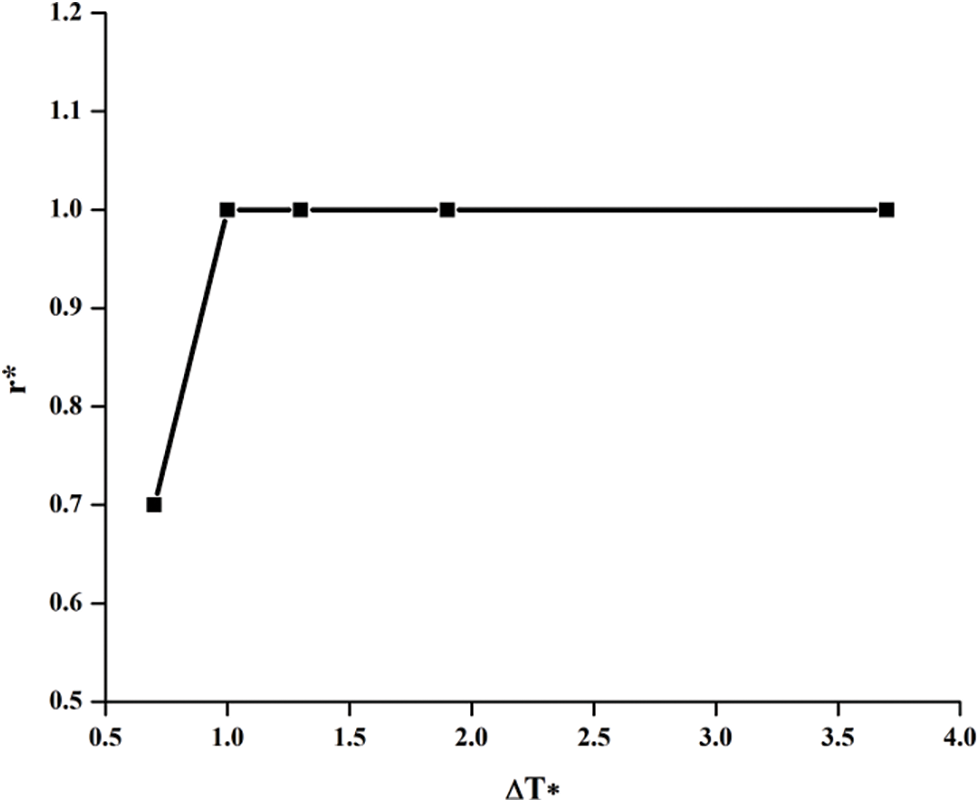
Figure 19: Plot of r* against ΔT* for nitrogen at 37.35 bar

(Nux)fcF3=0.275×(Rex)Ref0.505(Prref)0;371(T∞ΔT)0.033(20)

The R2 value with respect to Eq. (20) is found to be 0.998. The deviations are <5% for 525 data points (97.5%) out of 540 points and the remaining 15 points have deviations between 5 and 7 percent. In Eq. (20), T∞ appears explicitly and this is not desirable. Hence the dimensionless T∞ which appears in Eq. (20) is replaced by ∆T*. In that case the regression analysis yields.

(Nux)fcF3=0.277×(Rex)Ref0.505(Prref)0.386(ΔT∗)0.033(20a)

The R2 value with respect to Eq. (20a) is found to be 0.9984. Comparison of Nusselt numbers obtained using Eq. (20a) with the actual predictions indicates that only 4 data points out of 540 have deviations between 5 and 8 percent and the rest have deviations within ±5 percent.

(iv) Format with correlation based on enthalpy ratios (Format F4): This format, which uses enthalpy ratios in the correlation to account for the variation of fluid properties, has been used by Rousselet et al. [29] for predicting the Nusselt number based on their experimental results for free convection from horizontal cylinders to supercritical carbon dioxides. Further, they have proposed two correlations one for the cases for which Tw does not lie within the boundary layer (i.e., T∞ < Tw < T*) and the second correlation for cases for which Tw ≥ T*. The format of these two correlations is as follows:

(Nux)fc4a=a1(Rexb1)(Pr∞)c1(iwic)d1(ici∞)e1(21)

valid for cases for which T∞ < Tw < T*, and for cases for which Tw ≥ T* > T∞ the proposed correlation is of the form

(Nux)fc4b=a2(Rexb2)(Pr∞)c2(iwic)d2(ici∗−i∞)e2(22)

In the present investigation, 342 data points are available for which the condition Tw < T* is satisfied. Hence using the format given in Eq. (21), regression analysis yields the following:

(Nux)fcF4a=0.32×(Rex0.50)(Pr∞)0.049(iw∗ic∗)−0.033(ic∗i∞∗)0.013(23)

The R2 value with respect to Eq. (23) is found to be 0.9998. All the data points have deviations that are less than ±2%.

There are 198 data points for which the condition is Tw ≥ T*. Using Eq. (22) for these data points gives correlation as

(Nux)fcF4=0.21(Rex0.504)(Pr∞)1.049(iwic)−0.180(ici∗−i∞)−0.0837(24)

The R2 value with respect to Eq. (24) is 0.996. Only one data point has deviation >10% (=10.3%), 27 data points have deviations between 5% and 9% and the remaining points have deviations <5%.

(v) Format using constant property correlation with four property ratios (Format F5): In this format, the correlation for the Nusselt number for supercritical Nitrogen is expressed in terms of the Nusselt number for constant property fluids. If the four property ratios are used in the correlation, then this format will be of the form

(Nux)fcF5=0.942×((Nuxfccp)1.009×(Cp0.098)×(ρ∗)−0.022×(k∗))−0.121(25)

In Eq. (25), (Nux)xfccp represents the correlation for Nusselt number for laminar forced convection for constant property fluids and is given by [22,29]

(Nux)xfccp=0.332×Rex0.5×Pr∞0.3333)(26)

The R2 value with respect to Eq. (25) is found to be 0.9887. Out of 540 data points, only 6 points have deviations between 5 and 7 percent, and the rest have deviations less than 5%.

(vi) Format using constant property correlation with two property ratios (Format F6): In this format, the correlation for Nux is similar to Eq. (25), but has only two property ratios, namely, the specific heat ratio (C¯pCp∞) and the density ratio (ρ∞ρw). The regression analysis yields the correlation as

(Nux)xWBF6=0.926×((Nu)xfccp)1.009)×Cp∗0.1479×ρ∗−0.1589(27)

The R2 value with respect to Eq. (27) is found to be 0.8345. Only 4 data points have deviations between 5 and 8 percent and the rest of the points have deviations that are less than 5 percent.

(vi) Format using reference temperature concept and the dimensionless temperature ΔT* (Format F7T*). In the format F3 (Eq. (19)), the variation of the fluid properties is considered in the correlation by selecting a proper reference temperature to evaluate the fluid properties, in addition to the dimensionless temperature T∞/∆T. This dimensionless temperature has T∞ explicitly appearing in the correlation and this is not desirable. Instead, the dimensionless temperature, ∆T* (∆T* = [(T* − T∞)/∆T]) can be used. In that case, regression analysis yields the correlation as

(Nux)xfcF7=0.297×Reref0.505×Prref0.327×ΔT∗0.031(28)

The R2 value with respect to Eq. (28) is found to be 0.998. Only 4 data points out of 542 have deviations between 5% and 10% and the rest have deviations within ±5%.

6.2 Comparison of Correlations with the Actual Numerical Predictions for Forced Convection without Buoyancy Effects

The local heat transfer coefficients obtained using the correlations of various formats except the correlation based on enthalpy ratios, are compared with the actual numerical predictions. The reason for comparing the heat transfer coefficients and not the Nusselt numbers is because except for the reference temperature method, the fluid properties are evaluated at T∞ for other formats, whereas in the reference temperature format, the fluid properties required in the correlation are evaluated at the reference temperature which may or may not be the same as T∞. Table 3 shows the number of data points which have, (i) deviations that are >10%, (ii) the number of points with deviations between 5 and 10 percent, and (iii) the number of points with deviations ≤5%. It can be seen from this table that all formats of correlations predict local Nusselt numbers which agree with the actual predictions within ± ±10%. The correlations as per format fcF2, format fcF3, format fcF6 and format fcF7 predict Nusselt numbers that agree with the actual predictions within the ±5% for a maximum number of data points (99.26%) and hence recommended.

6.3 Correlations for Laminar Forced Convection with Buoyancy Effects

The procedure followed to find the correlations for laminar forced convection without buoyancy effects is also followed for forced convection with buoyancy effects except that an additional parameter Grx is introduced in the correlation in all the formats to account for the buoyancy effects.

(i) Format 8: This format is similar to format 1 (Eq. (13)) except that one more parameter Grx is introduced to account for the buoyancy effects. Thus, the format of the correlation is

(Nux)wbF1=a1(Rexb1)(Grx)c1(Pr)d1(C¯pCp\infty )e1(ρ∞ρw)f1(µ∞µw)g1(k∞kw)h1(29)

The constants a1 to h1 in Eq. (29) are obtained using multiple linear regression analysis for 540 data points and the correlation obtained is

(Nux)wbF1=0.481×(Rex0.528)(Grx)−0.008(Pr)−0.659(C¯pCp\infty )0.397(ρ∞ρw)−0.108(µ∞µw)−0.178(k∞kw)0.025(30)

The R2 value with respect to Eq. (30) is found to be 0.999. The deviations of the data points with respect to Eq. (30) are ≤2.5% for 520 data points (96.3%) out of 540 points and for the remaining 20 points the deviations lie between 2.5% and 6%.

(ii) Format 9: If it is assumed that the variation of viscosity and conductivity can be accounted for by using the density ratio and specific heat ratio in the correlation, then multiple linear regression analysis gives the following correlation:

(Nux)wbF2=0.298×(Rex0.554)(Grx)−0.017(Pr)0.011(C¯pCp\infty )0.171(ρ∞ρw)−0.153(31)

The R2 value with respect to Eq. (31), is found to be 0.998. For all the 540 data points the deviations are ≤5%.

(iii) Format 9.1 (Correlation using reference temperature method): In this format, for forced convection with buoyancy effects, the correlation is assumed to be of the form

(Nux)wbF3∗=a2(Grx)Refb2(Rex)Refc2(Prref)d2(T∞ΔT)e2(32)

In Eq. (32), all the dimensionless numbers, namely, (Grx)Ref, (Rex)Ref, Prref and (Nux)WBF9 are first calculated for all the data points using some reference temperature, say Tref = T∞ and using multiple linear regression analysis, the constants a2 to e2 are found. The constants are found to be as follows:

a2 = 0.383; b2 = 0.00042; c2 = 0.504; d2 = −0.399; e2 = 0.062.

Then r* which is the optimum value of r is found for each Δ* and for each pressure and the plot of r* vs. ΔT* is obtained. It has been found that for all pressure except p = 44.145 bar, the value of r* = 1 for all values of ΔT* and hence the plot of r* vs. ΔT* is shown in Fig. 20, only for p = 44.145 bar. From this plot r* can be obtained for any ΔT* and using Eq. (16) the reference temperature is determined to get the fluid properties at that temperature. Then the final form of correlation obtained is

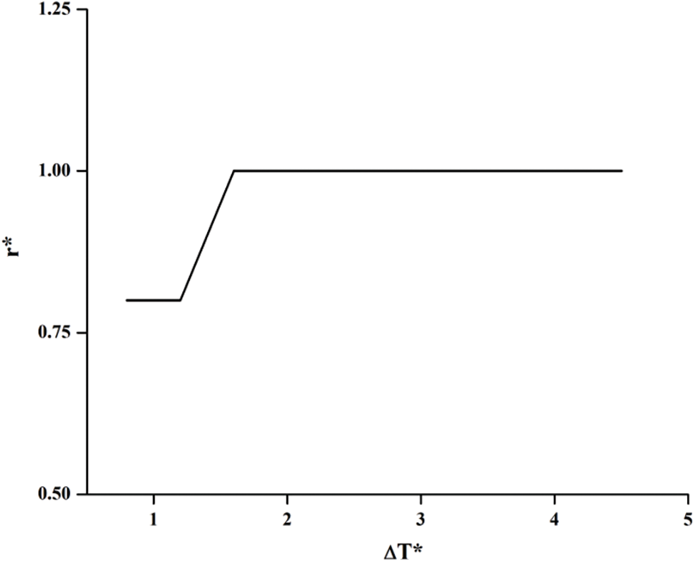
Figure 20: Plot of r* vs. ΔT* for nitrogen at 44.145 bar

(Nux)wbF3=0.383(Grx)Ref0.00042(Rex)Ref0.504(Prref)−0.399(T∞ΔT)0.062(33)

The R2 value with respect to Eq. (33), is found to be 0.996. It is found that 523 data points (96.9%) out of 540 points have deviations <5% and the remaining 17 data points have deviations between 5% and 10%. T∞ explicitly appears in Eq. (33) and this is not desirable. Instead, if dimensionless temperature ∆T* is used in the correlation, then regression analysis yields the correlation as

(Nux)wbF3∗=0.383(Grx)Ref0.00042(Rex)Ref0.504(33a)

The R2 value with respect to Eq. (33a) is found to be 0.995412. The Nusselt number predicted using Eq. (33a) agrees with the actual numerical predictions within ±5 percent for 497 points out of 537 points, and for the rest of the data points, the deviations are between 5 and 10 percent.

(iv) Format 10 (Correlation using enthalpy ratios): In this format, two correlations are proposed, one for the cases for which the data points have Tw < T* (cases for which T* lies outside the boundary layer) and the other correlation for which Tw ≥ T* (cases for which T* lies inside the boundary layer).

In the present investigation, 342 data points have Tw < T* and the format of the correlation is

(Nux)wbF4a=a3(Grxb3)(Rexc3)(Pr∞)d3(iw∗ic∗)e3(ic∗i∞∗)f3(34)

Regression analysis, using 342 data points, Eq. (34) reduces to

(Nux)wbF4=0.245×Grx−0.0068×Rex0.5242×Pr∞0.246×((iw∗ic∗)−0.028)×((ic∗i∞∗)−0.028)(35)

with R2 = 0.9992. Nusselt numbers predicted using Eq. (33) agrees with the actual numerical predictions within ±2 percent. For the case of remaining 198 data points for which Tw ≥ T*, the correlation is assumed to be of the form of

(Nux)wbF4=a3(Grxb3)(Rexc3)(Pr∞)d3(iw∗ic∗)e3(ic∗i∗∗−i∞∗)f3(36)

Regression analysis using Eq. (36) for these 198 points yields the correlation as

(Nux)wbF4=0.696×(Grx−0.0006)×(Rex0.521)×(Pr∞−1.231)×(iw∗ic∗)−0.156×(ic∗i∗∗−i∞∗)0.405(37)

with R2 = 0.994. Comparison of Nusselt numbers obtained using Eq. (37) with the actual numerical predictions indicate that 10 data points out of 197 points have deviations between 6% and 7% and the rest of data points have deviations less than 6%.

(v) Format 11 (Correlation using constant property correlation and four property ratios):

In this format, the correlation for the Nusselt number is expressed in terms of the correlation for constant property fluids with additional parameters to account for the variation of the fluid properties. Thus, the correlation takes the form

(Nux)wbF5=a4((Nux)mccp)b4(C¯pCp\infty )c4(ρ∞ρw)d4(µ∞µw)e4(k∞kw)f4(38)

In Eq. (38), (Nux)mccp represents the local Nusselt number for constant property fluids for mixed convection from a horizontal isothermal plate with heated surface facing downwards and is given by [29]

(Nux)WBcp=((Nux)fccp3+(Nux)nccp3)1/3(39)

In Eq. (39), (Nux)fccp represents local Nusselt number for forced convection for laminar flow over a flat plate for constant property fluids and (Nux)nccp represents the local Nusselt number for free convection for laminar flow over a horizontal isothermal flat plate with the heated surface facing downwards. The Nusselt numbers (Nux)fccp and (Nux)nccp are given by [29]

(Nux)WBF5=0.2025×(Grx∗Pr∞)0.25(40)

(Nux)fccp and (Nux)nccp are calculated for each data point and substituted in Eq. (39) to get (Nux)mccp for each data point and using these values along with Eq. (38) regression analysis is carried out to get the correlations as

(Nux)WBF5=1.16×((Nux)WBcp)0.961(C¯pCp\infty )0.339(ρ∞ρw)−0.048(µ∞µw)−0.204(k∞kw)−0.033(41)

The R2 value concerning Eq. (41) is found to be 0.996. Comparison of Nusselt number obtained using.

Eq. (41) with the actual numerical predictions indicates that 3 data points (0.56%) have deviations >10%, 12 data points (2.22%) have deviations between 5% and 10% and the rest (97.22%) have deviations <5%.

(vi) Format 12 (Correlation using constant property correlation with only two property ratios):

This format assumes that the nature of the variation of viscosity and thermal conductivity are similar to the variations of density and specific heat for supercritical fluids and hence the specific heat ratio and the density ratio will also account for the variation of viscosity and thermal conductivity. The multiple linear regression analysis for this format yields the following correlation:

(Nux)WBF6=0.926×((Nux)WBcp0.990187)×(Cp∗0.123848)×(ρ∗−0.1635)(42)

The R2 value concerning Eq. (42) is found to be 0.999969. Eq. (42) predicts the Nusselt numbers which are within ±5% for 515 out of 537 data points and the rest of the data points the deviations are between 5 and 15%.

(vii) Format 12 (Correlation using constant property correlation and ∆T*): For this format, regression analysis yields the correlation as

(Nux)WBF7∗=((Nuref)WBcp)0.973139×(ΔT∗)0.075684(43)

The R2 value concerning Eq. (43) is found to be 0.999948. The Nusselt numbers predicted by Eq. (43) agree with the actual numerical predictions within ±5% for 497 out of 537 data points and for the rest of the data points the deviations are between 5% and 15%.

6.4 Comparison of Correlations with the Actual Numerical Predictions for Forced Convection with Buoyancy Effects

All the correlations except the correlation based on enthalpy ratios are compared with the actual numerical predictions. The comparison shown in Fig. 21 is based on heat transfer coefficients and not on the Nusselt numbers as explained earlier and is due to the fact that except for the reference temperature method, the fluid properties are evaluated at T∞ for other formats, whereas in the reference temperature format, the fluid properties required in the correlation are evaluated at the reference temperature which may or may not be the same as T∞. The correlation based on enthalpy ratios is not included in this comparison as, under this format, two separate correlations based on enthalpy ratios are proposed in this comparison, one for the cases for which Tw < T* and the other correlation for cases for which Tw ≥ T*. Fig. 21 indicates that except for 6 data points (1.11%), the ratio of hx based on the correlation to hx obtained in actual numerical predictions varies between 0.9 and 1.1. In other words, the local heat transfer coefficients obtained by various correlations agree with the actual numerical predictions within ±10%. Table 4 shows the number of data points that have (i) deviations that are >10%, (ii) the number of points with deviations between 5% and 10%, and (iii) the number of points with deviations ≤5%. It can be seen from this table that all formats of correlations predict local Nusselt numbers which agree with the actual predictions within ±10%. The correlations as per format 7 and format 8 predict Nusselt numbers which agree with the actual predictions within ±5% for a maximum number of data points (99.44% of data points) and hence recommended.

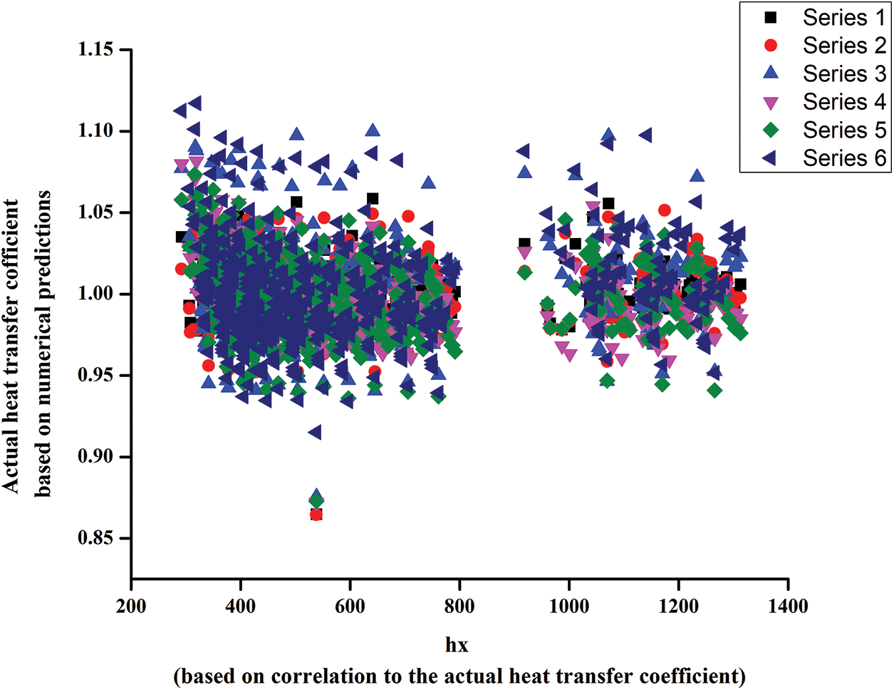
Figure 21: Plot of the ratio of hx based on correlation to the actual heat transfer coefficient against the actual heat transfer coefficient based on numerical predictions for forced convection with buoyancy effects

7  Conclusions

Numerical predictions for laminar forced convection heat transfer with and without significant buoyancy effects from an isothermally heated horizontal flat plate to supercritical nitrogen are presented. A data pool of 540 points has been used both for convection with and without buoyancy effects, by varying the ambient pressure, wall temperature, and free stream velocity. The flow has been categorized based on the dimensionless number GrxRex2, forced convection without buoyancy effects [GrxRex2<0.1] and with buoyancy effects [0.1≤GrxRex2≤10]. The wall temperatures were chosen in such a manner that all three conditions Tw<T∗, Tw=T∗ and Tw>T∗ were covered. Using all the data points obtained, four different formats of correlations are proposed to predict the Nusselt numbers for forced convection without buoyancy effects, and the heat transfer coefficients obtained by using these correlations are compared with the actual numerical predictions and the agreement is found to be satisfactory. Similarly, for forced convection with buoyancy effects, three different formats of correlations for local Nusselt numbers have been proposed and compared with the actual numerical predictions. This comparison is based on the local heat transfer coefficient and the agreement is found to be satisfactory. The comparison for both cases indicates that the correlation involving all four property ratios is best suited for predicting the Nusselt number with and without buoyancy effects.

Acknowledgement: We would like to thank Manipal Institute of Technology Bengaluru, Manipal Academy of Higher Education, Manipal, India, for the invaluable support throughout the research process.

Funding Statement: The authors received no specific funding for this study.

Author Contributions: The authors confirm their contribution to the paper as follows: study conception and design: T. R. Seetharam, K. S. Rajendra Prasad; data collection: Sathya Sai; analysis and interpretation of results: Sathya Sai, K. S. Rajendra Prasad, Adithya Garimella; draft manuscript preparation: Adithya Garimella, K. S. Rajendra Prasad. All authors reviewed the results and approved the final version of the manuscript.

Availability of Data and Materials: All the information/data necessary for the work is provided in the manuscript itself.

Conflicts of Interest: The authors declare that they have no conflicts of interest to report regarding the present study.

References

1. Knez, Ž., Markočič, E., Leitgeb, M., Primožič, M., Hrnčič, M. K. et al. (2014). Industrial applications of supercritical fluids: A review. Energy, 77, 235–243. https://doi.org/10.1016/j.energy.2014.07.044 [Google Scholar] [CrossRef]

2. Hall, W. B. (1974). Heat transfer under supercritical pressures. International Heat Transfer Conference Digital Library, Begel House Inc. [Google Scholar]

3. Kakac, S. (1987). The effect of temperature-dependent fluid properties in convective heat transfer. In: Handbook of single-phase convective heat transfer, pp. 1–56. John Wiley & Sons. [Google Scholar]

4. Polyakov, A. F. (1991). Heat transfer under supercritical pressures. Advances in Heat Transfer, 21, 1–53. https://doi.org/10.1016/S0065-2717(08)70333-2 [Google Scholar] [CrossRef]

5. Pioro, I. L., Hussam, F. K., Romney, B. D. (2004). Heat transfer to supercritical fluids flowing in channels—empirical correlations (survey). Nuclear Engineering and Design, 230(1–3), 69–91. [Google Scholar]

6. Fritsch, C. A., Grosh, R. J. (1961). Free convection heat transfer to n supercritical fluid. Proceedings of the 1961 International Heat Transfer Conference, Boulder, Colorado. [Google Scholar]

7. Hasegawa, S., Yoshioka, K. (1966). An analysis for free convective heat transfer to supercritical fluids. International Heat Transfer Conference Digital Library, Chicago, Begel House Inc. [Google Scholar]

8. Kato, H., Niichi, N., Masaru, H. (1968). Studies on the heat transfer of fluids at a supercritical pressure: 1st report, a proposition of reference values of thermal properties and experiments with supercritical Carbon-Dioxide. Bulletin of JSME, 11(46), 654–663. https://doi.org/10.1299/jsme1958.11.654 [Google Scholar] [CrossRef]

9. Nishikawa, K., Ito, T. (1969). An analysis of free convective heat transfer from an isothermal vertical plate to supercritical fluids. International Journal of Heat and Mass Transfer, 12(11), 1449–1463. https://doi.org/10.1016/0017-9310(69)90027-1 [Google Scholar] [CrossRef]

10. Nowak, E. S., Konanur, A. K. (1970). An analytical investigation of free convective heat transfer to supercritical water. Journal of Heat Transfer, 92, 345–350. https://doi.org/10.1115/1.3449669 [Google Scholar] [CrossRef]

11. Seetharam, T. R., Sharma, G. K. (1977). Numerical prediction of free convective heat transfer from vertical isothermal surfaces to fluids in the near-critical region. Proceedings of Fourth National Heat and Mass Transfer Conference, pp. 273–279. Roorkee, India. [Google Scholar]

12. Deshpande, G. S., Sharma, G. K. (1979). Theoretical investigation of natural convection heat transfer to supercritical helium under constant wall-heat flux condition. Fourth National Symposium on Cryogenics, pp. 47–52. Bombay, India. [Google Scholar]

13. Seetharam, T. R., Sharma, G. K. (1979). Free convective heat transfer to fluids in the near-critical region from vertical surfaces with uniform heat flux. International Journal of Heat and Mass Transfer, 22(1), 13–20. https://doi.org/10.1016/0017-9310(79)90093-0 [Google Scholar] [CrossRef]

14. Seetharam, T. R., Sharma, G. K. (1982). Heat transfer by turbulent free convection from a plane vertical surface to near-critical carbon-di-oxide. International Heat Transfer Conference Digital Library, Begel House Inc., Germany. [Google Scholar]

15. Simoneau, R. J. (1977). Velocity and temperature profiles in near-critical nitrogen flowing past a horizontal flat plate. National Heat Transfer Conference, Salt Lake City, Utah. [Google Scholar]

16. Graham, R. W., Simoneau, R. J., Williams, J. C. III (1971). Velocity and temperature profiles in near critical nitrogen. NASA Technical Memorandum, No. NASA-TM-X-52988. [Google Scholar]

17. Sri Sathya Sai, S. V., Ranganath, R., Shane Shaju, T. R. S., Seetharamu, K. N. (2021). Numerical predictions of forced convection and free convection heat transfer from an isothermal horizontal flat plate to supercritical nitrogen. Thermal Science and Engineering Progress, 23, 100867. https://doi.org/10.1016/j.tsep.2021.100867 [Google Scholar] [CrossRef]

18. Lemmon, E. W., Huber, M. L., McLinden, M. O. (2002). NIST reference fluid thermodynamic and transport properties–REFPROP. NIST Standard Reference Database 23. [Google Scholar]

19. Martorell, I., Herrero, J., Grau, F. X. (2003). Natural convection from narrow horizontal plates at moderate Rayleigh numbers. International Journal of Heat and Mass Transfer, 46(13), 2389–2402. https://doi.org/10.1016/S0017-9310(03)00010-3 [Google Scholar] [CrossRef]

20. Corcione, M. (2008). Natural convection heat transfer above heated horizontal surfaces. International Conference on Heat and Mass Transfer, pp. 206–243. Acapulco, Mexico. [Google Scholar]

21. Linstrom, P. J., Mallard, W. G. (2001). The NIST Chemistry WebBook: A chemical data resource on the internet. Journal of Chemical & Engineering Data, 46(5), 1059–1063. https://doi.org/10.1021/je000236i [Google Scholar] [CrossRef]

22. Incropera, F. P., DeWitt, D. P., Bergman, T. L., Lavine, A. S. (1996). Fundamentals of heat and mass transfer, vol. 6. New York: Wiley. [Google Scholar]

23. Cengel, Y., Cimbala, J. (2013). Ebook: Fluid mechanics fundamentals and applications (si units). McGraw Hill, India. [Google Scholar]

24. Bringer, R. P., Smith, J. M. (1957). Heat transfer in the critical region. AIChE Journal, 3(1), 49–55. https://doi.org/10.1002/aic.v3:1 [Google Scholar] [CrossRef]

25. Fluent, A. (2011). Fluent 14.0 user’s guide. Ansys Fluent Inc, USA. [Google Scholar]

26. Gustavo, J., Otero, R., Ashish, P., Diez, R., Pecnik, R. (2018). Turbulence modelling for flows with strong variations in thermo-physical properties. International Journal of Heat and Fluid Flow, 73, 114–123. https://doi.org/10.1016/j.ijheatfluidflow.2018.07.005 [Google Scholar] [CrossRef]

27. Ghorbani-Tari, S., Ghajar, A. J. (1985). Improved free convective heat-transfer correlations in the near-critical region. AIAA Journal, 23(10), 1647–1649. https://doi.org/10.2514/3.9144 [Google Scholar] [CrossRef]

28. Ghajar, A. J., Parker, J. D. (1981). Reference temperatures for supercritical laminar free convection on a vertical flate plate. Journal of Heat Transfer, 103, 613. https://doi.org/10.1115/1.3244516 [Google Scholar] [CrossRef]

29. Rousselet, Y., Warrier, G. R., Dhir, V. K. (2013). Natural convection from horizontal cylinders at near-critical pressures—part I: Experimental study. Journal of Heat Transfer, 135(2), 022501. https://doi.org/10.1115/1.4007672 [Google Scholar] [CrossRef]