Amplitude and Period Effect on Heat Transfer in an Enclosure with Sinusoidal Heating from Below Using Lattice Boltzmann Method

Nomenclature

1  Introduction

Natural convection is a widely observed phenomenon found in various systems, such as residential heating and cooling, heating circuits, and electronic devices [1–4]. Typically, this phenomenon arises from either variable or constant heating of a fluid. Many researchers have investigated and simulated such convection, employing diverse numerical methods to tackle complex problems (e.g., FDM: Finite Difference Method, FVM: Finite Volume Method, LBM: Lattice Boltzmann Method). A well-established benchmark solution for laminar natural convection of air within a square cavity was presented by de Vahl Davis [5]. Le Quéré [6] provided accurate solutions for a square cavity subjected to high Ra. Oliveira et al. [7] employed the FVM to address turbulent natural convection in square enclosures, incorporating large eddy simulation (LES). In their study, the lateral surfaces of the enclosure were maintained at different isothermal temperatures, while the upper and lower surfaces were thermally isolated. The investigation focused on Ra = 1.58109. Salat et al. [8] conducted a comparative result between experimental and numerical cases of turbulent flows in a differentially heated cavity. They demonstrated a good agreement between experimental results and numerical methods of mean temperature and vertical velocity. Numerous researchers have utilized the Lattice Boltzmann Method (LBM) to simulate various natural convection phenomena [9–13] and for complex geometry [14–17]. Some authors based on natural convection in the square enclosure, Mohamad et al. [18,19] evaluated LBM capability to simulate 2D natural convection in cavities by comparing LBM outcomes with those of FDM. They elucidated the necessary steps for utilizing LBM in natural convection problems. A comprehensive evaluation of forcing schemes within the lattice Boltzmann method (LBM) [20]. Rashidi [21] employed a proficient finite element approach to discretize the continuous system of depth equations, enabling the numerical simulation of shallow water wave propagation. Recent works by Abouricha et al. [22–25] adopted LBM to simulate natural convection in a square cavity heated from below at a constant temperature. As the Ra increased, they observed a substantial rise in heat transfer, a pattern also observed in the heat source size (Lr). For variable heating regimes, Abourida et al. [26] explored natural convection in a square cavity with horizontally heated walls subjected to different heating models, utilizing finite difference techniques. Their study encompassed a range of Rayleigh numbers (5 × 105 ≤ Ra ≤ 106) and revealed the influence of heating frequency on heat transfer, streamlines, and isotherms. They observed non-periodic solutions at higher Rayleigh numbers. Wang et al. [27] studied the impact of temperature-dependent properties on the natural convection of power-law nanofluids in rectangular cavities featuring sinusoidal temperature distributions. Nabwey [28] employed a set of analytical methods wherein the primary partial differential equations governing the flow were transformed into nonlinear ordinary differential equations (ODEs). This transformation was undertaken to investigate the heat and mass transfer characteristics of a non-Newtonian nanofluid flowing towards a vertically stretched surface. Most prior studies focused on cavities with heating walls maintained at constant (or periodically varying) temperatures or heat fluxes, employing numerical methods like FDM, FVM and FEM. Or based on the effect of physical or geometric parameters on the heat transfer [29–31]. Therefore, the current study aims to explore how varying the amplitude and period of heating temperature impacts heat transfer, flow structure, and temperature distribution within the cavity core using the simulation by lattice Boltzmann method (LBM), all while maintaining a fixed Ra.

2  Physical Configuration and Method

2.1 Physical Configuration

In this particular study, the LBM was employed to replicate the phenomenon of heat transfer through natural convection, incorporating the element of variable heating. The investigation revolves around a 2D enclosure (Fig. 1, left) filled with air characterized by a Pr = 0.71. The cavity, with a side length denoted as H, experiences heating from beneath, achieved by imposing a temperature denoted as θh (Fig. 1, right) on a specific section measuring L = 0.8H, strategically positioned at the center of the lower wall. One of the vertical walls features a cold segment indicated by θc = 0, whereas the remaining walls maintain adiabatic conditions. This configuration can simulate a small-scale test room (home shower), equipped with a solar water heater. The water circulating through the floor generates heat at varying temperatures over time, depending on the day and night.

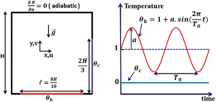
Figure 1: Physical geometry (left) and thermal excitations (right)

2.2 Lattice Boltzmann Method (LBM)

The LB framework utilized in this context aligns with the one applied in prior studies [22,24]. This model leverages a pair of distinct single-particle distribution functions: fk(x,t) for addressing dynamic aspects and gk(x,t) for simulating thermal fields. Hence, the approach corresponds to the LBM referred to as model D2Q9, characterized by its two-dimensional nature and incorporation of nine discrete velocities, as illustrated in Fig. 2.

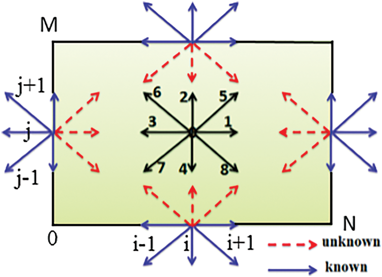
Figure 2: LBM model used D2Q9

The lattice Boltzmann equation under the BGK approximation and in the absence of external forces can be expressed as stated in references [22,32,33]:

∂fk∂t+ck∂fk∂x=−1τm(fk−fkeq)(1)

The equilibrium distribution can be expressed mathematically by the following expression [34]:

fkeq(x,t)=ωkρ(x,t)(1+3ckuc2+92(cku)2c4−32u2c2)(2)

where c=ΔxΔt is the lattice speed, Δx=1 is the lattice space, and Δt=1 is the lattice time.

For D2Q9 (Fig. 2), the discrete velocities ck are defined as follows:

c0=(0,0), c1−4=(±1,0);(0,±1) and c5−8=(±1,±1)

The weights factors ωk are given by: ω0=49, ω1−4=19 and ω5−8=136

Finally, the BGK approximation for the LB equation discretized and simplified with external forces can be written as:

fk(x+ckΔt,t+Δt)=(1−wm)fk(x,t)+wmfkeq(x,t)+ΔtFk(3)

For momentum wm is prescribed through kinematic viscosity as:

wm=Δtτm=13ν+0.5(4)

Taking into account the Boussinesq approximation, the external force denoted as Fk in Eq. (3) is expressed as follows:

Fk=3ωkρgβΔT.ckc2(5)

Finally, for the model D2Q9, the density ρ and velocity u, are calculated by summing moments within the velocity space as follows:

ρ(x,t)=∑k=0k=8fk(x,t)(6)

ρu(x,t)=∑k=0k=8ckfk(x,t)(7)

For the temperature, other distribution functions for the lattice Boltzmann method are defined as:

gk(x+ckΔt,t+Δt)=(1−ws)gk(x,t)+wsgkeq(x,t)(8)

where ws is associated to the diffusion coefficient as:

ws=Δtτs=13α+0.5(9)

The equilibrium distribution functions for the temperature can be used at first-order [35].

gkeq=ωkT(x,t)[1+3ckuc2](10)

The temperature T(x,t) is calculated by using the summation:

T(x,t)=∑08gk(x,t)(11)

2.3 Boundary Conditions

The boundary conditions pertaining to the investigated problem are outlined below:

•   Dynamic boundary conditions:

For all the walls: u=v=0

•   Thermal boundary conditions:

The dimensionless temperature can be defined as:

θ=T−TcTh−Tc(12)

On the adiabatic walls, we used this condition ∂θ∂n=0, where n is the normal of walls. The numerical approximation used for the top wall:

gk(i,M)=gk(i,M−1)(13)

Here, i denotes the iteration index along the x direction, while signifies the count of lattice points situated on the upper wall as indicated in Fig. 2.

For the imposed temperature on the hot and the cold portion, the bounce-back conditions can be used:

gk=(ωk+ωopp(k))θ−gopp(k)(14)

For example: (opp(1)=3; opp(2)=4; opp(6)=8)

On the cold portion: θc=0

On the hot portion: θh=1+a.sin(2πT0t)

2.4 Nusselt Number

The Nusselt number at the hot part can be calculated by the expression below:

Nu¯=−108∫110910∂θ∂y|y=0dx(15)

3  Test of Numerical Method and Code

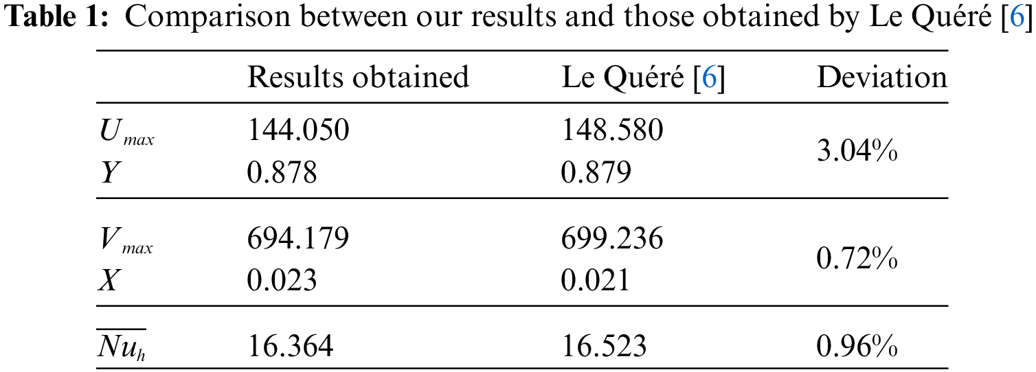
The FORTRAN code implemented in this study was validated and tested through a comparison of the outcomes against those reported by Le Quéré [6] for Ra = 107. Fig. 3 represents the configuration used for this validation. It is a differentially heated square cavity filled with air. In Table 1, a juxtaposition was made between the highest x-velocity value along the vertical midpoint (Umax), the highest y-velocity value along the horizontal midpoint (Vmax), and the mean Nusselt number (Nu¯). The analysis of this comparison highlights a favorable concurrence, with a maximum discrepancy not surpassing 3.04%.

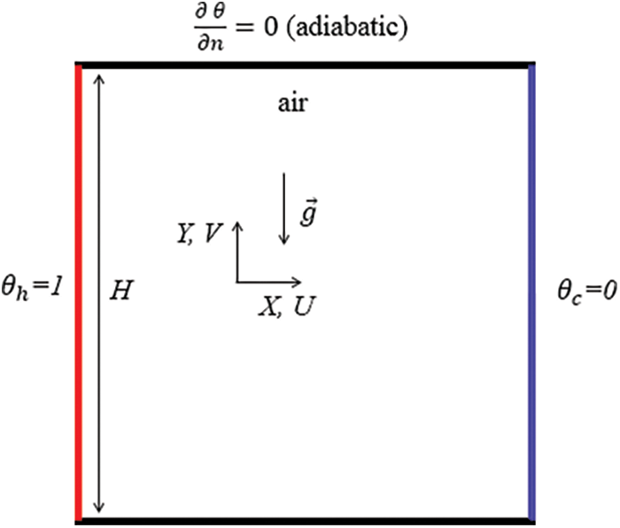
Figure 3: Square cavity differentially heated [6,36]

4  Results and Discussion

In the following section, the flow structures, temperature fields and heat transfer rates are inspected for divers values in the series of amplitude 0.2 ≤ a ≤ 0.8 and for double values of period T0 and T′0 = 2 × T0, by using air (Pr = 0.71), a fixed Rayleigh numbers Ra = 107. Numerically in two dimensions, we have divided the physical domain into N = 210 nodes along the x axis, and M = 210 along the y axis. The stability of the numerical method used, the constraints of divergence code FORTRAN, and computing time are taken into consideration. We need the term gβ figured in the expression of Rayleigh number, gβ=Ra(αν)/(ΔTH3). Considering the lattice unit and the stability of the LBM, for example, we choose the kinematic viscosity ν=0.02, or another value less than 0.1. Based on the law of similarity and dimensionless numbers, Pr=0.71=ν/α, then the thermal diffusivity α = 0.02/0.71. By replacing ΔT by Δθ and H by M, we can calculate gβ=Ra(αν)/(M3) figured in Eq. (5).

Notice that the model is dimensionless, and all results will be presented in dimensionless forms and discussed in the last periods.

4.1 Streamlines and Isotherms

The effect of the variation of the amplitude “a” on the thermal field and dynamic field is represented in Fig. 4, in the form of isotherms (above) and streamlines (below). We have examined the solution during one period To at t = nTo + To/i, where i = 1,2,3,… and n ≥ 5. We notice that at every moment, we have a different solution by the fact that the imposed temperature varies as a sinusoidal function of time and can be minimal or maximum, which causes the change in the form of thermal field.

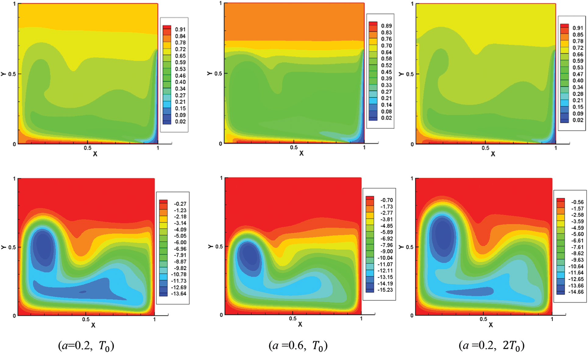
Figure 4: Isotherms (above) and streamlines (below) for the amplitude a = 0.2 and a = 0.6 at time calculation 8.105 steps

The examination of the isotherms shows that thermal stratification is generated near to the hot walls and at the top of the cavity when Y ≥ 0.75, the dimensionless temperature is set around 0.71. Elevating both the amplitude and period results in an observed rise in temperature within the central region of the cavity, which is shown in Figs. 5 and 6. The examination of the streamlines shows that there is a dissymmetrical location of the cells and the flow is formed by a large cell contains small cells, more or less hot, rotates clockwise because the cold air decent near the right vertical wall pushing the hot air to continued rotation. Generally, the structure form of the flow does not change by the variation of the amplitude and the period, but it changes over time during a period t = n.T0 + T0/i.

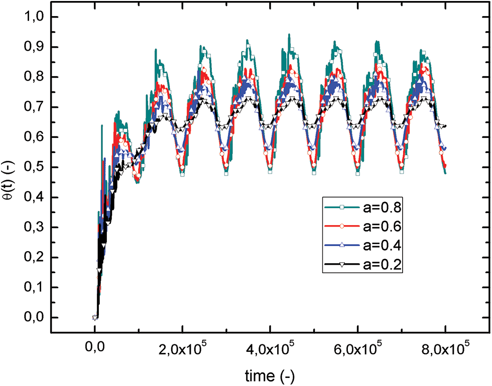
Figure 5: Temperature evolution at the center (X = 0.5;Y = 0.5) for various amplitudes “a”

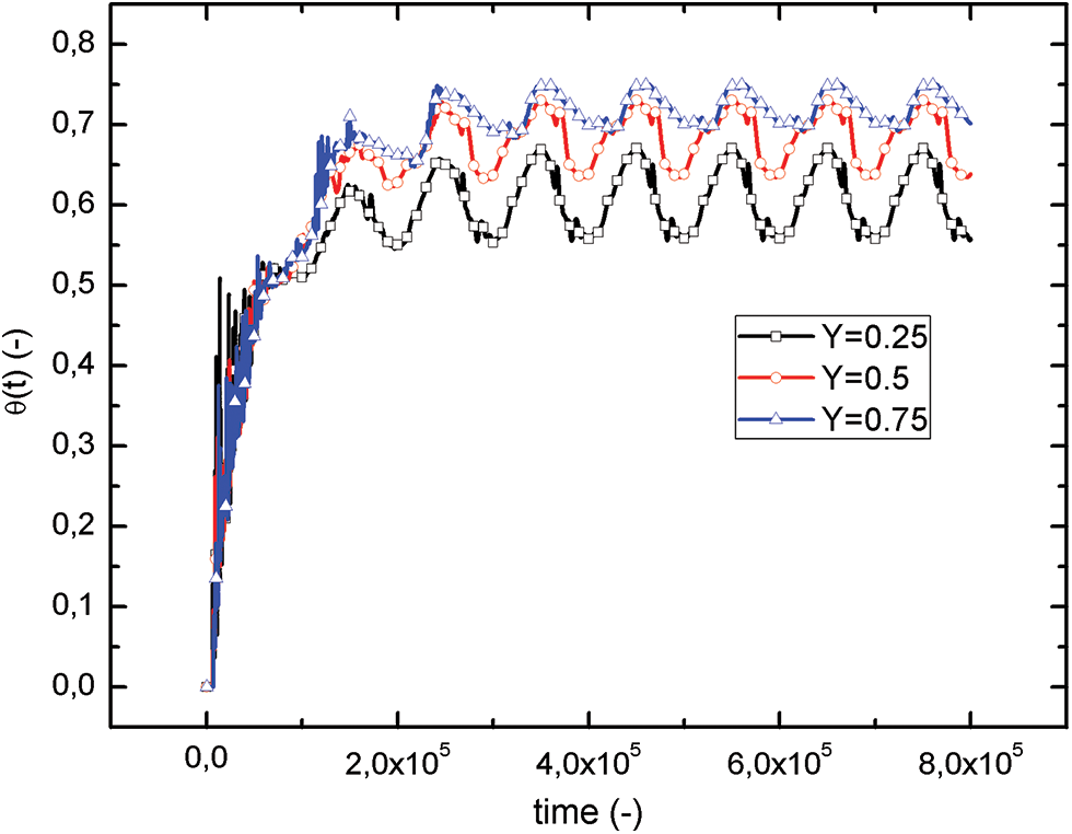
Figure 6: Evolution of temperature for different position along the vertical centerline X = 0.5

Note that these figures are represented at the final instant of the calculation time 8.105 = 8T0 = 4T0'. Apparently, at times t = nT0 and n = 5,6,7,8, the change in isotherms and streamlines is very weak. On the other hand, at times t = nT0 + T0/i and i = 1.2,3,… there is a change but is not covered in this paper.

4.2 Temperature Profiles

The temporal variations of dimensionless temperatures, denoted as θ(t), are depicted in Fig. 5 at the center of the enclosure for different values of the amplitude “a” of the imposed temperature. θh, and in Fig. 6 for the following positions Y = 0.25; 0.5; 0.75 of the vertical mid plan X = 0.5, for an amplitude a = 0.2. Normally, the temperature at the heart of the cavity does not vary in phase with the imposed temperature. This is because of the time delay in heat transfer from one area to another.

For all values of the amplitude “a” of the θh, the dimensionless temperature θ(t) at the center oscillates periodically around 0.66. Its amplitude increases with the increase of the amplitude “a” and becomes disturbed for the reason of the turbulent flow in the center of the cavity. For the amplitudes 0.2 and 0.8, the temperature oscillates in the margin [0.63; 0.73] and [0.48; 0.88], respectively (Fig. 5). The examination shows that θ(t) preserves the same periodicity with θh and increases towards a maximum value when θh > 1 and decreases near a minimal value while θh < 1 due to the important hot air movement when θh > 1 that one has heating in this case and cooling in the other case θh < 1.

Fig. 6 shows that the temperatures on the vertical medium axis for an amplitude a = 0.2 oscillate periodically in the range [0.55; 0.75] around different mean values (0.61, 0.69 and 0.72 for Y = 0.25, Y = 0.5 and Y = 0.75, respectively). The oscillation amplitudes are very significant towards the bottom of the cavity and decrease as one goes upwards (when Y increases). When Y is superior strictly to 0.75, the evolution of θ(t) approaches asymptotically towards very close values that appear in the upper third of the cavity, as already mentioned in the isothermal lines.

In Fig. 7, we present the evolution of θ(t) at the center of the enclosures for the amplitude 0.2 and for double values of the period T0 and T0’ = 2 × T0, in directive to evaluate the period effect of θh on the temperature inside the cavity. From these results, it is remarkable that the amplitude of θ(t) at the center of the enclosures is affected by the period variation of θh. It shows that the amplitude of θ(t) at the center of the enclosures increases by increasing the period of θh. This is due to the heating and cooling time, which increases for longer periods.

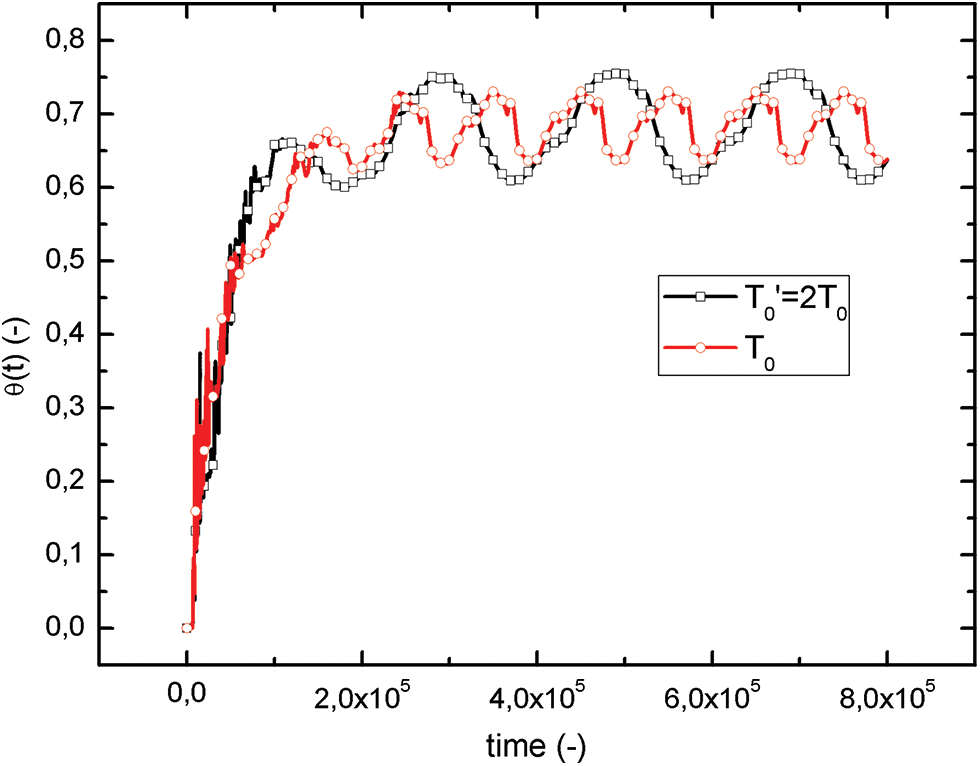
Figure 7: Period effect on temperature evolution at the center (X = 0.5; Y = 0.5) for a = 0.2

The time evolution of the dimensionless temperature θ(t) at the center of the square enclosures is shown in Fig. 8, for an amplitude of the imposed temperature in the range 0.2 ≤ a ≤ 0.8. The temperature oscillates between a maximum θmax and minimum θmin around a mean value. This maximum can be correlated with the amplitude “a” in the linear form. After fitting the curve, for Ra = 107 and 0.2 ≤ a ≤ 0.8, the correlation between θmax And “a” can be written as:

θmax=0,27×a+0,66(16)

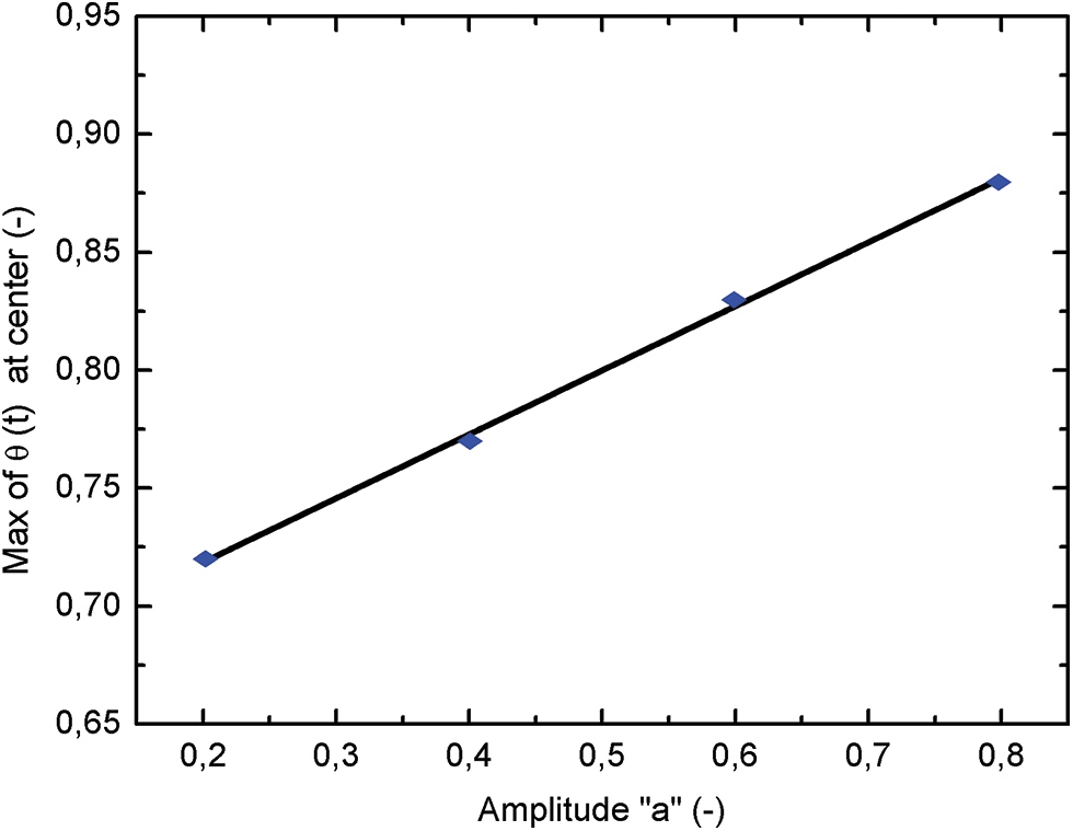
Figure 8: Maximum variation of the temperature at the center with amplitude “a”

This correlation gives an idea of the maximum temperature, or Expected temperature value at the center of the cavity for heating conditions already specified.

4.3 Heat Transfer

The investigation of heat transfer within the enclosures involves computing the Nusselt number (Nu¯) on the heated portion. The variation of this parameter is displayed in Fig. 9, for different values of amplitude “a” and for double values of the period of θh. In general, an increase in the amplitude “a” leads to an enhancement in the heat transfer, as indicated by the Nusselt number within the enclosure. The evolution of Nu¯ continue periodic and oscillate in phase with θh about a mean value equivalent to 12. We noticed that when “a” increases the amplitude of Nu¯ similarly increases, this latter varied in the margin of 7 ≤ Nu¯(t) ≤ 15 for a = 0.2 and between of 0 ≤ Nu¯(t) ≤ 30 for a = 0.8. We observed that when θh maximal causes a disturbance of solution, unlike when this layer is minimal, that is due to the turbulent flow of air in the core of the enclosure, and its maximum is nearly doubled when “a” doubled. Note well when θh is minimal and the amplitude “a” higher, the heat transfer does not exist as the amplitude a = 0.8.

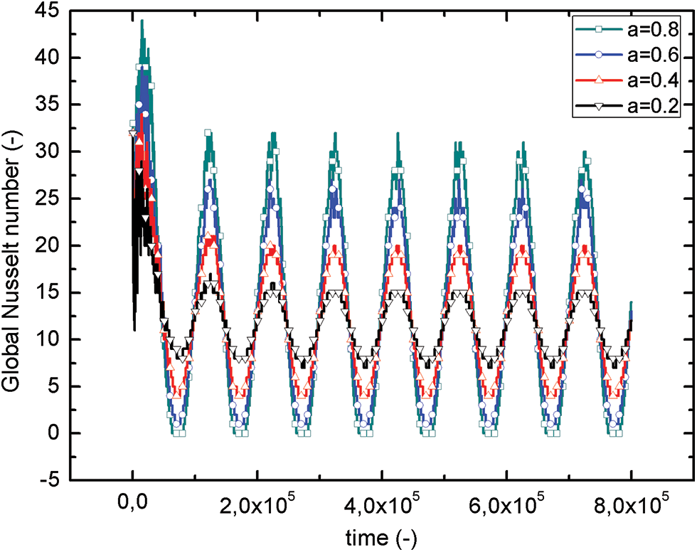
Figure 9: Amplitude “a” effect on global Nusselt number evolution on the hot portion

Fig. 10 shows the temporal evolution of the Nu¯ for a = 0.2, and for two values of the period T0 and T0’ = 2 × T0. From these obtained results, it can be deduced that the amplitude of the Nusselt number (Nu¯) is not affected by the deviation of the period. But it keeps the same periodicity and always remains in phase with the imposed temperature θh.

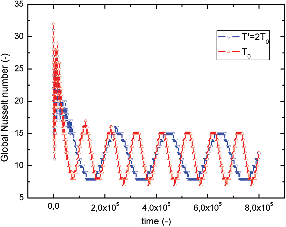
Figure 10: Period effect on global Nusselt number evolution on the hot portion for a = 0.2

Generally, when heating is maintained at a constant temperature, during the steady-state phase, the temporal evolution of the average Nusselt number exhibits a consistent value for low Rayleigh numbers (Ra). However, for higher Ra values, it tends to oscillate around a mean value. This is due to the appearance of the phenomena of transition to turbulence and the calculation method of Nusselt number Nu¯ (single or double precision). In this case, the number of Ra used is 107 and the heating is non-uniform. We observe at each step that there is a zigzag appearing in the evolution of the global Nusselt number represented in Figs. 8 and 9. Given that the number of calculation time steps is higher, the evolution appears as a trapezoidal wave.

The global Nusselt number oscillates around an average value with a maximum Nu¯max and minimum Nu¯min. For Ra = 107 and in the range of the amplitude 0.2 ≤ a ≤ 0.8, the maximum of the global Nusselt number Nu¯max varies linearly with “a”. After fitting the curve in Fig. 11, this relation can be written as:

Nu¯max=24×a+10(17)

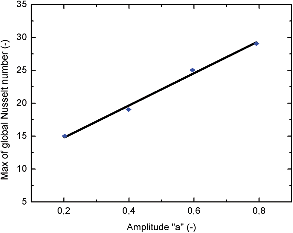
Figure 11: Maximum variation of the global Nussselt number with amplitude “a”

This correlation is used to estimate the maximum of heat transfer in the enclosure for a well-determined heating rate.

5  Conclusion

In this article, we have conducted a numerical solution of heat transfer to analyze the effect of sinusoidal heating from below on the thermal field, dynamic field and Nusselt number Nu¯ by using the lattice Boltzmann method for Ra = 107. The Results found in this work show that:

•   An increase in amplitude “a” increases the maximum of θ(t) in the core of the enclosure and the heat transfer.

•   Increasing the parameter “a” results in an amplification of the forces propelling the cells upwards, leading to the emergence of upward-moving air puffs that rotate around their own axes.

•   The time evolution of Nu¯ continue periodic and oscillate in phase with θh about a mean value.

•   The variation of the period of θh has a significant consequence on the amplitude of θ(t) in the core of the enclosure; this end upsurges when the period “T0” increases.

•   The Nusselt number Nu¯ is approximately not affected by the variation of the period “T0”.

•   In the range of amplitudes 0.2 ≤ a ≤ 0.8 we have established the following correlations between the amplitude of the θh and the maximum of θ(t) at the center and the global Nusselt number:

For temperature: θmax=0,27×a+0,66

For Nusselt number: Nu¯max=24×a+10

Acknowledgement: The authors wish to express their gratitude to the National Center for Scientific and Technical Research (CNRST) for granting access to computational resources.

Funding Statement: The authors received no specific funding for this study.

Author Contributions: All authors played a role in shaping the study's concept and design. The tasks of material preparation, data collection, and analysis were carried out by Noureddine Abouricha; Chouaib Ennawaoui and Mustapha El Alami. The initial draft of the manuscript was written by Noureddine Abouricha, and all authors provided feedback on earlier iterations of the document. Subsequently, all authors reviewed and endorsed the final version of the manuscript.

Availability of Data and Materials: Data will be made available on request.

Conflicts of Interest: The authors declare that they have no conflicts of interest to report regarding the present study.

References

1. Chu, T. Y., Hickox, C. E. (1990). Thermal convection with large viscosity variation in an enclosure with localized heating. Journal of Heat Transfer, 112, 388–395. [Google Scholar]

2. Tanda, G. (1997). Natural convection heat transfer in vertical channels with and without transverse square ribs. International Journal of Heat and Mass Transfer, 40(9), 2173–2185. [Google Scholar]

3. Sajjadi, H., Gorji, M., Hosseinizadeh, S. F., Kefayati, G. R., Ganji, D. D. (2011). Numerical analysis of turbulent natural convection in square cavity using Large-Eddy Simulation in Lattice Boltzmann Method. Iranian Journal of Science and Technology. Transactions of Mechanical Engineering, 35(M2), 133–142. [Google Scholar]

4. Chen, S. (2009). A large-eddy-based lattice Boltzmann model for turbulent flow simulation. Applied Mathematics and Computation, 215(2), 591–598. [Google Scholar]

5. de Vahl Davis, G. (1983). Natural convection of air in a square cavity: A bench mark numerical solution. International Journal for Numerical Methods in Fluids, 3(3), 249–264. [Google Scholar]

6. Le Quéré, P. (1991). Accurate solutions to the square thermally driven cavity at high Rayleigh number. Computers & Fluids, 20(1), 29–41. [Google Scholar]

7. Oliveira, M., Menon, G. J. (2002). Simulação de grandes escalas utilizada para convecção natural turbulenta em cavidades. Proceedings of the ENCIT 9th Congresso Brasileiro de Engenharia e Ciências Térmicas, pp. 1–11. Caxambu, Brazil, CD. [Google Scholar]

8. Salat, J., Xin, S., Joubert, P., Sergent, A., Penot, F. et al. (2004). Experimental and numerical investigation of turbulent natural convection in a large air-filled cavity. International Journal of Heat and Fluid Flow, 25(5), 824–832. [Google Scholar]

9. Imani, G. (2020). Lattice Boltzmann method for conjugate natural convection with heat generation on non-uniform meshes. Computers & Mathematics with Applications, 79(4), 1188–1207. [Google Scholar]

10. Baliti, J., Elguennouni, Y., Hssikou, M., Alaoui, M. (2022). Simulation of natural convection by multirelaxation time lattice Boltzmann method in a triangular enclosure. Fluids, 7(2), 74. [Google Scholar]

11. Astanina, M. S., Ghalambaz, M., Chamkha, A. J., Sheremet, M. A. (2021). Thermal convection in a cubical region saturated with a temperature-dependent viscosity fluid under the non-uniform temperature profile at vertical wall. International Communications in Heat and Mass Transfer, 126, 105442. [Google Scholar]

12. Wang, L., Yang, X., Huang, C., Chai, Z., Shi, B. (2019). Hybrid lattice Boltzmann-TVD simulation of natural convection of nanofluids in a partially heated square cavity using Buongiorno's model. Applied Thermal Engineering, 146, 318–327. [Google Scholar]

13. Astanina, M. S., Sheremet, M. A. (2023). Numerical study of natural convection of fluid with temperature-dependent viscosity inside a porous cube under non-uniform heating using local thermal non-equilibrium approach. International Journal of Thermofluids, 17, 100266. [Google Scholar]

14. Wang, L., Zhao, Y., Yang, X., Shi, B., Chai, Z. (2019). A lattice Boltzmann analysis of the conjugate natural convection in a square enclosure with a circular cylinder. Applied Mathematical Modelling, 71, 31–44. [Google Scholar]

15. Polasanapalli, S. R. G., Anupindi, K. (2019). A high-order compact finite-difference lattice Boltzmann method for simulation of natural convection. Computers & Fluids, 181, 259–282. [Google Scholar]

16. Polasanapalli, S. R. G., Anupindi, K. (2022). Mixed convection heat transfer in a two-dimensional annular cavity using an off-lattice Boltzmann method. International Journal of Thermal Sciences, 179, 107677. [Google Scholar]

17. Li, X. Y., Zhang, H., Liu, J., Wang, Q., Ma, T. (2018). Gravity effect on natural convection melting investigated with 2D and 3D lattice Boltzmann methods. International Heat Transfer Conference 16, Beijing, China, Begel House Inc. [Google Scholar]

18. Mohamad, A. A., Kuzmin, A. L. E. X. A. N. D. R. (2010). A critical evaluation of force term in lattice Boltzmann method, natural convection problem. International Journal of Heat and Mass Transfer, 53(5–6), 990–996. [Google Scholar]

19. Mohamad, A. A., El-Ganaoui, M., Bennacer, R. (2009). Lattice Boltzmann simulation of natural convection in an open ended cavity. International Journal of Thermal Sciences, 48(10), 1870–1875. [Google Scholar]

20. Bawazeer, S. A., Baakeem, S. S., Mohamad, A. A. (2021). A critical review of forcing schemes in lattice boltzmann method: 1993–2019. Archives of Computational Methods in Engineering, 28, 4405–4423. [Google Scholar]

21. Rashidi, F. (2016). An efficient finite element method for numerical modeling of shallow water wave propagation. International Journal of Intelligent Engineering and Systems, 9(3), 156–162. https://doi.org/10.22266/ijies2016.0930.16 [Google Scholar] [CrossRef]

22. Abouricha, N., El Alami, M., Kriraa, M., Souhar, K. (2017). Lattice boltzmann method for natural convection flows in a full scale cavity heated from Below. American Journal of Heat and Mass Transfer, 4(2), 121–135. [Google Scholar]

23. Abouricha, N., Alami, M. E., Souhar, K. (2016). Numerical study of heat transfer by natural convection in a large-scale cavity heated from below. 2016 International Renewable and Sustainable Energy Conference (IRSEC), pp. 565–570. Marrakech, Morocco, IEEE. [Google Scholar]

24. Abouricha, N., El Alami, M., Gounni, A. (2019). Lattice Boltzmann modeling of natural convection in a large-scale cavity heated from below by a centered source. Journal of Heat Transfer, 141(6), 062501. [Google Scholar]

25. Noureddine, A., Mustapha, E. A. (2021). Heat source size effect on heat transfer in a local heated from below at high Rayleigh number. AIP Conference Proceedings, vol. 2345. ENSA Khouribga, Morocco, AIP Publishing. [Google Scholar]

26. Abourida, B., Hasnaoui, M., Douamna, S. (1999). Transient natural convection in a square enclosure with horizontal walls submitted to periodic temperatures. Numerical Heat Transfer, Part A: Applications, 36(7), 737–750. [Google Scholar]

27. Wang, L., Huang, C., Yang, X., Chai, Z., Shi, B. (2019). Effects of temperature-dependent properties on natural convection of power-law nanofluids in rectangular cavities with sinusoidal temperature distribution. International Journal of Heat and Mass Transfer, 128, 688–699. [Google Scholar]

28. Nabwey, H. A. (2020). Integration of Group method analysis and rough sets theory to investigate heat and mass transfer of the flow of a non-newtonian nanofluid towards a vertical stretching surface. International Journal of Intelligent Engineering & Systems, 13(6), 393–403. https://doi.org/10.22266/ijies2020.1231.35 [Google Scholar] [CrossRef]

29. Njoroge, J., Gao, P.(2022). Geometry contributions to natural convection heat transfer enhancement by the chimney effect. IOP Conference Series: Earth and Environmental Science, vol. 983, 012039. IOP Publishing. [Google Scholar]

30. Mahdi, M. S., Khadom, A. A., Mahood, H. B., Yaqup, M. A. R., Hussain, J. M. et al. (2019). Effect of fin geometry on natural convection heat transfer in electrical distribution transformer: Numerical study and experimental validation. Thermal Science and Engineering Progress, 14, 100414. [Google Scholar]

31. Fereidooni, J. (2022). The effect of fins and wavy geometry on natural convection heat transfer of TiO2 water nanofluid in trash bin-shaped cavity. The European Physical Journal Special Topics, 231(13), 2713–2731. [Google Scholar]

32. Succi, S. (2001). The lattice Boltzmann for fluid dynamics and beyond. Oxford University, UK. [Google Scholar]

33. Ganzarolli, M. M., Milanez, L. F. (1995). Natural convection in rectangular enclosures heated from below and symmetrically cooled from the sides. International Journal of Heat and Mass Transfer, 38(6), 1063–1073. [Google Scholar]

34. He, Y. L., Liu, Q., Li, Q., Tao, W. Q. (2019). Lattice Boltzmann methods for single-phase and solid-liquid phase-change heat transfer in porous media: A review. International Journal of Heat and Mass Transfer, 129, 160–197. [Google Scholar]

35. Kefayati, G. R. (2013). Lattice Boltzmann simulation of MHD natural convection in a nanofluid-filled cavity with sinusoidal temperature distribution. Powder Technology, 243, 171–183. [Google Scholar]

36. Dixit, H. N., Babu, V. (2006). Simulation of high Rayleigh number natural convection in a square cavity using the lattice Boltzmann method. International Journal of Heat and Mass Transfer, 49(3–4), 727–739. [Google Scholar]