A Chart-Based Diagnostic Model for Tight Gas Reservoirs Based on Shut-in Pressure during Hydraulic Fracturing

1  Introduction

There are abundant tight gas resources with reservoirs characterized by low porosity, low permeability, and poor connectivity. Horizontal wells and hydraulic fracturing are essential technical means for the efficient development of these tight gas resources [1–3]. Post-fracture fracture diagnosis and evaluation are the main methods for assessing fracturing effects and are important bases for optimizing fracturing designs and processes. Currently, fracture monitoring and diagnosis technologies mainly include acoustic logging, seismic and microseismic monitoring, resistivity logging, and nuclear magnetic resonance [4–6]. These technologies play important roles in fracture monitoring and diagnosis, but they also have drawbacks such as complex data interpretation, limited resolution, high costs, and depth restrictions [7–10]. Compared to other fracture monitoring and diagnosis technologies, the analysis of shut-in pump pressure curves based on hydraulic fracturing construction has broad application prospects owing to advantages such as monitoring data being unaffected by construction and the capability to obtain multiple parameters [11,12].

Currently, the theoretical basis for shut-in pump pressure fracture diagnosis in hydraulic fracturing relies mainly on the dimensionless G-function model over time established by Nolte [13] based on the Carter leak-off equation. However, in this model, symmetric bilaterally fractured fractures are assumed and parameters related to natural fracture closure pressure drops are treated as constants, limiting its applicability in evaluating complex artificial fracture networks [14–16]. In response to the post-fracture diagnosis of complex fracture networks, extensive research has been conducted and many interpretations have been proposed for shut-in pump pressure fracture diagnosis [17,18]. Barree et al. [19] improved the G-function diagnostic method based on the Nolte model to identify more complex nonidealized fracture features, proposing pressure analysis using the G-function, square root of time, and double logarithmic plots for micro-injection pressure loss tests. Castillo [20] proposed a new G-function chart based on the G-function to judge fracture closure and suggested changes in the leak-off coefficient related to pressure during the fracture closure process. Liu et al. [21] provided corresponding analytical and semi-analytical solutions for behaviors such as tip extension, pressure loss, and multiple closures before closure in micro-injection pressure loss tests. Liu et al. [22] used the slope of a composite G-function chart to determine closure points and calculate fracture parameters, while Mohamed et al. [23] and Mohamed et al. [24] divided the flow stage using double logarithmic methods, plotted double logarithmic charts using shut-in time and pressure data, divided them into three stages, and effectively identified fracture closure points by combining double logarithmic charts with G-function charts. However, current interpretation methods mainly entail analysis of shut-in pump pressure data from small-scale micro-injection pressure loss tests, with limited research being conducted on shut-in pump pressure fracture diagnosis for large-scale hydraulic fracturing communicating with complex fracture networks in tight reservoirs.

To address the issue of decreasing fracture flexibility and area with natural fracture closure caused by hydraulic fracturing communicating with natural fractures in tight gas reservoirs, a theoretical model for shut-in pump pressure fracture diagnosis was established, with the geometric morphology of communicating natural fractures and the variation of leak-off volume with time under various leak-off mechanisms taken into account. Modern mathematical physics methods and Python programming were applied to solve the theoretical model, and G-function charts were drawn. By overlaying the G-function during the natural fracture closure period with pressure derivative curves, the influence of fracture parameters such as leak-off coefficient, area, closure pressure, and time on chart characteristics was discussed. This led to the development of a new model and analysis method for accurately diagnosing fracture step or constant-rate closure during pressure attenuation after hydraulic fracturing, which is critical for improving post-fracturing production capacity evaluation in tight gas reservoirs. Example analysis was conducted using on-site fracturing pressure monitoring data to verify the applicability and reliability of this method in post-fracture diagnosis of complex fracture networks in tight gas reservoirs.

2  Analysis of Shut-in Pump Pressure Theoretical Model

Nolte and co-workers Nolte [25] and Nolte et al. [26] proposed the classic G-function model for post-fracturing evaluation of symmetric bilaterally fractured fractures based on the material balance equation of fracturing fluid injection; this can be used to determine the closure time and closure pressure of fractures. The model assumptions are as follows: (1) The fracturing fluid is incompressible, so the volume of fracturing fluid pumped in equals the volume lost to the formation and the volume involved in fracturing. (2) The leak-off coefficient of the fracturing fluid is constant and unaffected by pressure changes, as described by the Carter leak-off modele. (3) The fracture area remains constant after well shut-in. (4) The fracture flexibility is constant and linearly related to fracture width and pressure. (5) The fracture height and closure pressure remain constant after well shut-in.

The relationship between net fracture pressure and fracture flexibility, as well as the relationship among net fracture pressure, fracture closure pressure, and fluid pressure within the fracture, can be described as follows:

(1)

(2)

(3)

where represents the fracture compliance (in m/MPa), represents the average width of the fracture (in meters), represents the net pressure within the fracture (in megapascals), represents the fluid pressure within the fracture (in megapascals), represents the closure pressure of the fracture (in megapascals), and represents the pressure at the end of pumping (in megapascals).

The average width of the fracture can be expressed as , where represents the surface area of the fracture when pumping is stopped (in m2) and represents the volume of the fracture when pumping is stopped (in m3). Differentiating Eq. (2) with respect to time gives the time derivatives of the fracture volume, fracture compliance, and surface area of the fracture when pumping is stopped:

(4)

Nolte [13] established the material balance equation for an incompressible fracturing fluid: , where represents the volume of the pumped fluid (in m3) and represents the volume of fluid lost (in m3). Based on the assumption that is considered constant, by differentiating Vi with respect to time t and substituting into Eq. (4), the relationship among pressure, fracture volume, and loss volume can be obtained:

(5)

The Carter [27] leak-off equation quantifies the leak-off rate on one side of the fracture as , where is the fracture leak-off coefficient (in m/min0.5) and vL is the leak-off rate of the fracturing fluid (in m/min). Assuming that the fracture opens and begins to leak-off after time τ, and taking the differential element of the fracture area as dA, we can obtain the differential form of the leak-off volume on one side of the fracture:

(6)

where represents the time for crack initiation (in minutes) and represents the pumping time (in minutes).

If negligible fluid losses are assumed, the rate of crack area growth is proportional to time with the formula , where is the crack area growth index (dimensionless) and is the single-side area of the crack (in m2). Integrating Eq. (6) yields the volume of filtrate during the pumping process. Normalizing the parameters leads to an expression for the dimensionless filtrate volume during the pumping process over dimensionless time. This quantifies the entire crack filtration process. The time during pumping and shut-in periods is denoted as , where the dimensionless time during pressure drop stages is defined as . This results in the overall dimensionless time filtrate volume, with the integral part defining the function for the total filtrate volume:

(7)

The total filtrate volume of the crack minus the filtrate volume during the pumping process equals the filtrate volume of the crack during shut-in periods:

(8)

Substituting into Eq. (5) yields the differential relationship between crack pressure and crack filtrate volume after shut-in:

(9)

(10)

Both and can be approximated by analytical solutions for the boundary values of filtration. By integrating Eq. (8), the following analytical expression for the crack pressure and crack filtrate volume after shut-in can be obtained:

(11)

The relevant expression for the G-function has been derived as

(12)

in which

(13)

(14)

where is the dimensionless G-function with respect to time, is the fitted pressure value (in megapascals), Δpw is the crack pressure after shut-in (in megapascals), is the crack filtrate coefficient (in m/min0.5), is the crack compliance (in m/MPa) and is the pumping time (in minutes).

Because the fracture filtration coefficient and fracture flexibility are considered unchanged in the model, is regarded as the slope value of Δpw (ΔtD) and V. Therefore, Castillo proposed that, if the pressure drop test stage is constant, then the fracture is in the closed stage. Laubach [17] also proposed adding the G curve to the diagnostic chart of the function curve to observe the fracture closure period more directly, showing that, when the fracture is closed, the curve will deviate from the characteristic curve. Taking the derivative of Eq. (12) and taking the first-order forward difference gives

(15)

3  Establishment of Pressure Fracture Diagnosis Model for Volume Fracturing Pump Shutdown

Fig. 1 shows that the basic theoretical model of pump shutdown pressure is the G-function diagram of a simple symmetrical double-wing fracture. The mass balance equation of a common G-function model considers only the fracture volume and fluid loss volume when the pump is shut down, without considering the communication of natural fractures. Therefore, it is not applicable to the complex situation of communication of natural fractures during the pumping process of tight reservoirs, as shown in Fig. 2. Therefore, on the basis of the above model, we further consider the influence of natural fractures on the filtration loss and establish a diagnosis model of pressure fractures in volumetric fracturing with a shut-down pump.

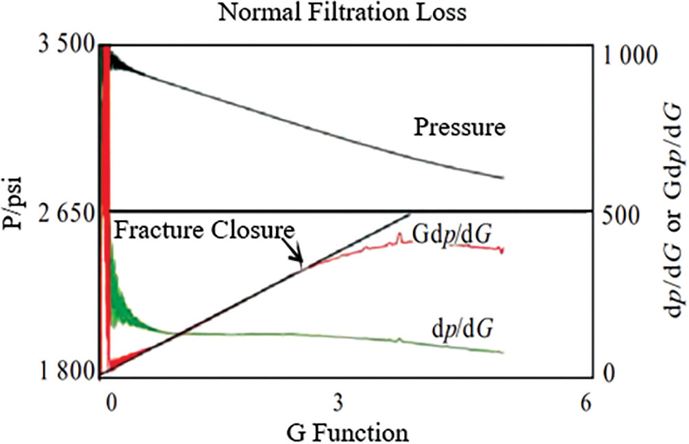
Figure 1: Common types of G-function charts

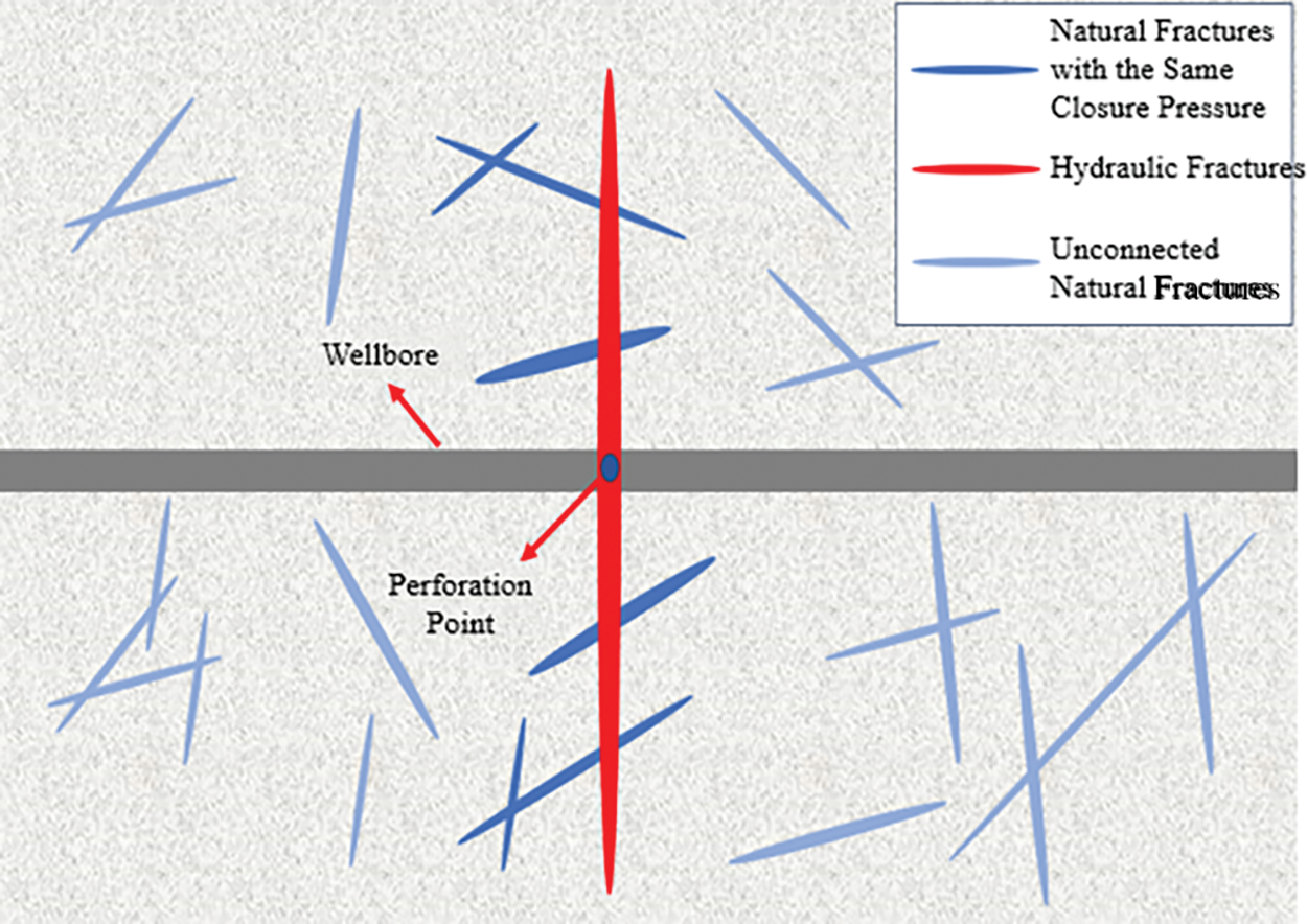
Figure 2: Physical model of natural fractures

The following assumptions were made in the model:

1. The fracturing fluid is incompressible, and the material balance states that the volume of fracturing fluid pumped equals the volume lost to the formation and the volume participating in fracture propagation.

2. Cater filtration is followed.

3. Prior to natural fracture closure, natural and hydraulic fractures jointly lose fluid to the reservoir. Fracture compliance and area are constants and are neglected after closure.

4. Fracture extension and friction are not considered during pumping and well shut-in processes.

The material balance equation states that the fluid volume during pumping equals the lost volume to the formation through the fractures and the fracture volume:

(16)

where represents the total filtrate volume of the hydraulic fractures (in m3), represents the volume of the hydraulic fractures (in m3), represents the total filtrate volume of the natural fractures (in m3), and represents the volume of the natural fractures (in m3).

Filtration follows Cater filtration, thus utilizing the formula for filtrate volume during shut-in periods. By considering the filtrate volumes of the hydraulic fractures and natural fractures separately through Eqs. (7) and (8), the total filtrate volume in the natural fractures and the total filtrate volume in the hydraulic fractures during the closure period can be determined:

(17)

Combining the relationship between fracture net pressure and fracture compliance yields the volumes of natural fractures and hydraulic fractures:

(18)

where represents the filtrate volume during the closure period of natural fractures (in m3), represents the filtration coefficient of natural fractures (in m/min0.5), represents the area of natural fractures (in m2), represents the closure time of natural fractures (dimensionless), represents the dimensionless time for hydraulic fracture closure, represents the filtration coefficient of hydraulic fractures (in m/min0.5), represents the area of hydraulic fractures (in m2), represents the closure time of hydraulic fractures (dimensionless), represents the width of hydraulic fractures (in meters), represents the compliance of hydraulic fractures (in m/min0.5), represents the closure pressure of hydraulic fractures (in megapascals), represents the area of natural fractures (in m2), represents the width of natural fractures (in meters), represents the compliance of natural fractures (in m/min0.5), and represents the closure pressure of natural fractures (in megapascals).

We then substitute the filtrate volumes and fracture volumes of natural fractures and hydraulic fractures into the material balance equation to get

(19)

By differentiating this equation with respect to , and based on the relationship among pressure, fracture volume, and filtrate volume, the expression for the pressure derivative during the closure period of natural fractures can be obtained:

(20)

Integrating this equation yields the expression for pressure drop before the closure of natural fractures:

(21)

As the pressure decreases and natural fractures completely close, only hydraulic fractures leak into the reservoir matrix. In Eq. (17), the material balance becomes . By substituting Eq. (18) into it, the equilibrium equation for hydraulic fractures during the pressure drop process can be derived:

(22)

Similarly, the expression for the overall pressure drop before the closure of hydraulic fractures can be obtained:

(23)

The expression for the pressure drop after the closure of natural fractures but before the closure of hydraulic fractures needs to consider the influence of the natural fracture closure period, which can be obtained from Eq. (23):

(24)

By combining Eqs. (23) and (24), the expression for the pressure drop of hydraulic fractures after the closure of natural fractures can be obtained, namely, the expression for the shut-in pressure of the fractures during volumetric fracturing:

(25)

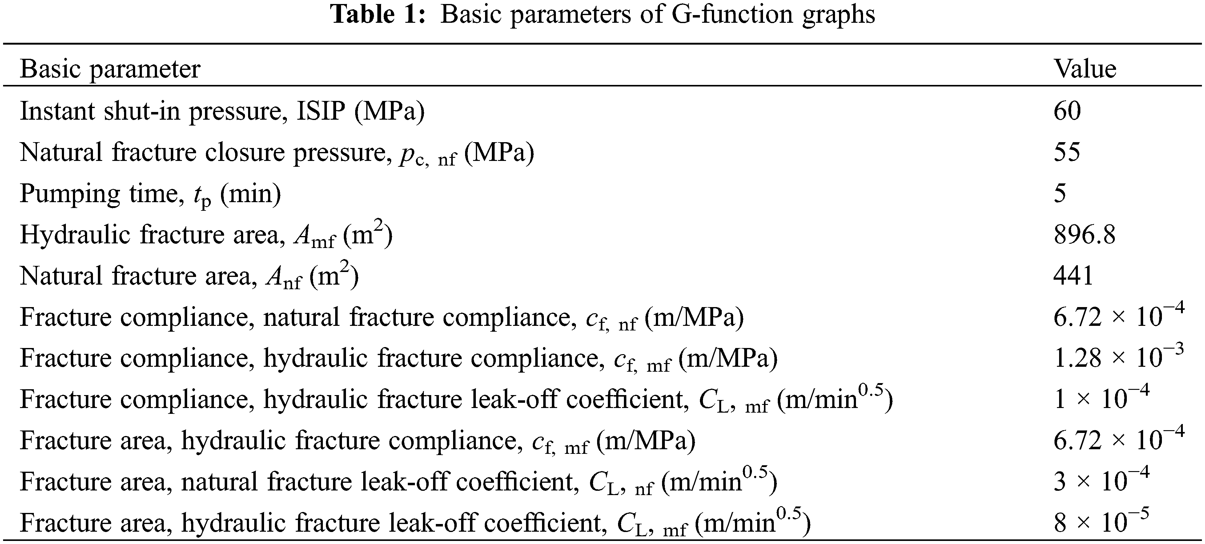
The following solving steps can be used to calculate the other parameters in Table 1, apart from the initial conditions:

1. Select initial conditions and and an appropriate .

2. Substitute the initial condition values into Eq. (25); iteratively, solve for . If the error is >0.01, readjust the step size of until the error is <0.01.

3. Calculate the values of , G-functions, and cumulative pressure derivatives corresponding to each .

4. Plot the G-function curve.

4  Characteristics and Analysis of the G-Function Plot in Volumetric Fracturing

4.1 Plotting and Features of the Graph

Fig. 3 illustrates the theoretical process of plotting the G-function model. Because the pressure drop equations before and after the closure of natural fractures differ, the closure pressure of natural fractures is initially used for differentiation. The pressure during the closure period of natural fractures is calculated using Eq. (21). When , the pressure during the closure period of hydraulic fractures is then calculated using Eq. (25), and finally, the G-function plot is drawn.

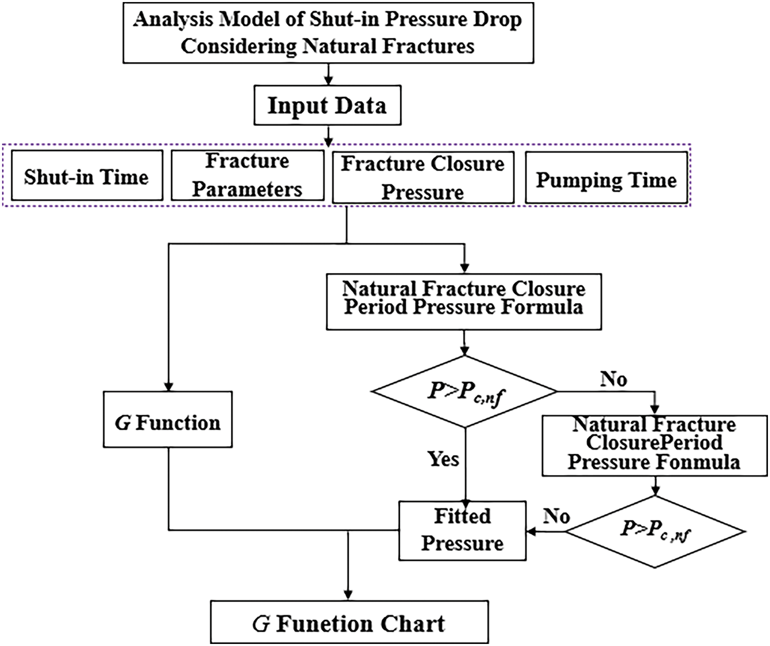
Figure 3: Program flowchart for calculating pump shutdown pressure considering natural fractures

Based on the pressure drop basic data in Table 1, the G-function plots for varying fracture compliance and fracture area can be drawn through hydraulic fracture pressure drop calculations, as shown in Figs. 4 and 5.

Figure 4: G-function chart of fracture flexibility with pressure variation

Figure 5: G-function chart of fracture area with pressure variation

During the natural fracture closure period and the process of fracture leak-off, the natural fractures do not participate in the leak-off. Additionally, there is some fluid at the contact surface of the natural fractures that does not leak into the reservoir. This results in a slower overall leak-off of the fractures and a smaller decrease in pressure. As a result, the G-function curve during the natural fracture closure period exhibits a concave trend, with the curve passing through the origin. The endpoint of the concave section corresponds to the pressure and time of natural fracture closure.

As hydraulic fractures and natural fractures leak off into the reservoir together, the overall leak-off of the fractures accelerates. This leads to a faster overall leak-off of the fractures and a greater decrease in pressure. Consequently, the G-function curve during the natural fracture closure period exhibits a “camelback” trend, with the curve passing through the origin. The endpoint of the camelback section corresponds to the pressure and time of natural fracture closure.

4.2 Parameter Sensitivity Analysis

A sensitivity analysis can be performed on the parameters , , and of natural fractures based on the G-function charts for fracture compliance and fracture area variations with pressure.

First, we consider fracture compliance values of 4.26 × 10−5, 6.72 × 10−4, and 1.27 × 10−3. In Fig. 6a, the concave feature of the natural fracture closure period G-function curve deepens. In contrast, for values of 3.2 × 10−3, 1.3 × 10−3, and 6.4 × 10−4, as shown in Fig. 6b, as the fracture compliance increases, the closure time of the natural fractures lengthens during the closure period, and the camelback feature of the G-function curve gradually converges, becoming a concave curve.

Figure 6: Analysis charts of variable fracture flexibility: (a) fracture compliance G-function chart; (b) fracture area G-function chart

Next we consider fracture area values of 620, 441, and 220 m2. As shown in Fig. 7a, as the fracture area increases, the closure time of the natural fractures lengthens, and the concave feature of the G-function curve during the natural fracture closure period deepens. In Fig. 7b, with increasing fracture area, the closure time of the natural fractures shortens, and the camelback feature of the G-function curve for natural fractures becomes more pronounced.

Figure 7: Analysis chart of variable fracture area: (a) fracture compliance G-function chart; (b) fracture area G-function chart

Finally, we consider control factor values of −10, 10, and 40. As shown in Fig. 8a, as the control factor increases, the closure time of the natural fractures lengthens, and the concave feature of the G-function curve during the natural fracture closure period deepens. In Fig. 8b, the camelback feature of the G-function curve during the natural fracture closure period converges as the control factor increases.

Figure 8: Analysis chart of variable control factors: (a) fracture compliance G-function chart; (b) fracture area G-function chart

Through the sensitivity analysis of , , and , it is evident that the G-function curve during the natural fracture closure period consistently exhibits a concave shape. As can be observed in Fig. 8, as fracture compliance, fracture area, and the control factor increase, the concavity of the G-function curve during the natural fracture closure period deepens.

5  Application Example and Analysis

Well Y is located in a tight gas reservoir area; the main lithology of the reservoir characterized by black and gray-black shales. The well was drilled to a total depth of 6870.0 m, with a vertical depth of 4345.43 m. The completion interval is in the Longmaxi Formation, with 139.7 mm casing used for completion and a horizontal section length of 2300.00 m.

Seismic multilevel fault data indicate the presence of natural fractures, with two sets of natural fracture zones developed along the well trajectory in intervals of 5860–6760 m (sections 2–14) and 5070–5160 m (sections 26–28), totaling 1016 m, as shown in Fig. 9.

Figure 9: Characteristics of natural fractures

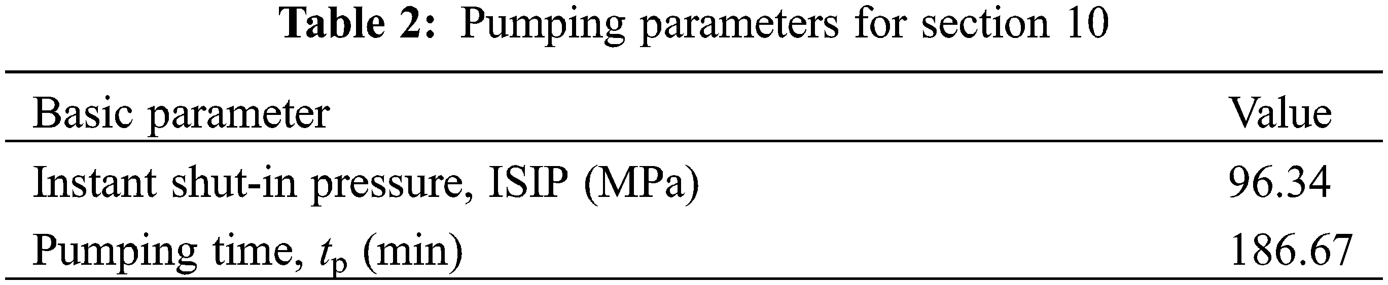
Based on the construction curve analysis (Fig. 10), the natural fracture zones in the 10th section are found to be widely distributed and complex, meeting the parameter requirements of the research model. Therefore, the 10th section in the interval of 5860–6760 m was selected for analysis, with a pumping time of 175.74 min and a shut-in pressure of 66.08 MPa.

Figure 10: Pressure curve for the 10th hydraulic fracturing operation

The input pumping parameters in the pressure drop calculation program are listed in Table 2.

5.1 Curve Fitting

Based on the actual G-function curve’s camelback feature, indicating the presence of single-level natural fractures, a shut-in pressure analysis model for single-level natural fractures related to pressure was selected. The final result obtained is the fitting of the G-function curve, as shown in Fig. 11.

Figure 11: G-function fitting chart for the 10th segment of Well Y

5.2 Fitting Results

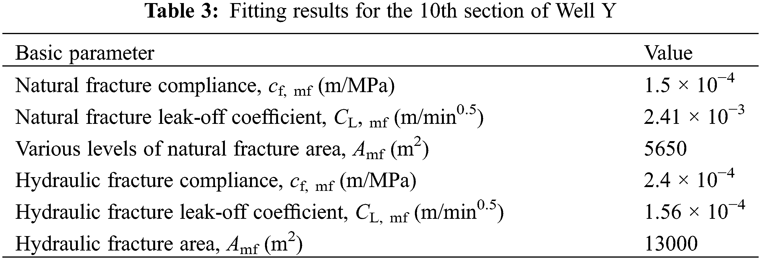
A single-level natural fracture was fitted, with closure pressures selected at 62.50 MPa. The hydraulic fracture closure pressure was determined to be 62.14 MPa, with a natural fracture leak-off coefficient of 0.00241 m/min0.5, reflecting a moderate rate of fluid loss through the communicating natural fractures per unit time. The average fracture compliance of each natural fracture level was calculated to be 0.00015 m/MPa, indicating a low degree of deformation under pressure for the communicating natural fractures. The total natural fracture area was determined to be 5650 m2, illustrating the presence of multiple communicating natural fractures during the pumping process, as listed in Table 3. The theoretical G-function of the modified section of section 10 of Well Y, calculated using the pressure drop model in this study, exhibited a good overall fit with the actual curve, validating the reliability and practicality of the model, as depicted in Fig. 11.

5.3 Reliability Analysis

As shown in Fig. 12, the Kelly Petroleum ant body fracture prediction interpretation indicates that fractures develop in well sections at depths of 4740–4868, 5026–5079, 5502–5534, 5959–6001, and 6418–6478 m. The ant body fracture prediction interpretation is similar to the interpretation results of Well Y in this study, with natural fractures developing in the 10th section.

Figure 12: Schematic diagram of ant body fracture prediction interpretation

Based on the interpretation results of Well Y and the reliability analysis, it can be concluded that the model for diagnosing complex fracture networks post-fracturing in this study is accurate and practical. This also suggests that, in the absence of geological mechanics data to interpret the degree of natural fracture development and fracture parameters, analysis can be conducted using the complex fracture network closure period fracture diagnostic method.

6  Conclusions

(1) A theoretical model for diagnosing fractures in volume fracturing shut-in pressures in tight gas reservoirs was established. G-function charts and natural fracture closure period G-function curves were plotted. The impact of fracture parameters such as leak-off coefficient, fracture area, closure pressure, and closure time on the chart features was discussed. The chart characteristics of the dynamic natural fracture formation shut-in pressure analysis model are as follows: The overlaid pressure derivative curve on the G-function chart exhibiting a concave or camelback trend indicates the natural fracture closure period, while the overlaid pressure derivative curve passing through the origin on the G-function chart represents the fracture closure period.

(2) By accurately identifying and obtaining parameters such as shut-in fracture pressure, natural fracture closure pressure, fracture compliance, and fracture area through the natural fracture closure period G-function curve, the sensitivity analysis of the chart to parameters was discussed. Parameters such as , , and of natural fractures were found to have a significant direct impact on the G-function chart. As fracture compliance and control factors increase or the leak-off coefficient decreases, the concave feature of the overlaid pressure derivative curve during the natural fracture closure period deepens, while the camelback feature converges. With an increase in fracture area, overall fracture leak-off slows, and the concave feature of the overlaid derivative curve during the natural fracture closure period on the G-function chart also deepens.

(3) In the example analysis, the instantaneous shut-in pressure fitted by the G-function chart showed a strong correlation with actual data, validating the reliability and applicability of the model. The fitting results of the example and the test data matched with an accuracy rate of >90% through the shut-in pressure fracture diagnostic model calculations, reflecting characteristics such as moderate fluid loss through communicating natural fractures per unit time, low deformation of fractures under pressure, and the presence of multiple communicating natural fractures during the pumping process in Well Y of a certain tight gas reservoir.

Acknowledgement: The authors would like to thank the reviewers and editors for their useful suggestions for improving the quality of our manuscript.

Funding Statement: The authors received no specific funding for this study.

Author Contributions: The authors confirm contribution to the paper as follows: Study conception and design: Mingqiang Wei and Neng Yang; data collection: Han Zou and Yonggang Duan; analysis and interpretation of results: Ahao Li, Han Zou and Mingqiang Wei; draft manuscript preparation: Neng Yang and Mingqiang Wei. All authors reviewed the results and approved the final version of the manuscript.

Availability of Data and Materials: Data will be made available on request.

Ethics Approval: Not applicable.

Conflicts of Interest: The authors declare no conflicts of interest to report regarding the present study.

References

1. Bauer M, Toth TM. Characterization and modelling of the fracture network in a Mesozoic karst reservoir: gomba oilfield, Paleogene basin, central Hungary. J Petrol Geol. 2017;40:319–34. doi:10.1111/jpg.12678. [Google Scholar] [CrossRef]

2. Li S, Liu D, Du C, Ma P, Li M, Gao H. Graphic template establishment and productivity evaluation model of post-fracturing based on the fluctuation pattern of G-function curve. Processes. 2023;11(6):1657. doi:10.3390/PR11061657. [Google Scholar] [CrossRef]

3. Peng Y, Luo A, Li YM, Wu YJ, Xu WJ, Sepehrnoori K. Fractional model for simulating long-term fracture conductivity decay of shale gas and its influences on the well production. Fuel. 2023;351:129052. doi:10.1016/J.FUEL.2023.129052. [Google Scholar] [CrossRef]

4. Peng Y, Zhao J, Sepehrnoori K, Li Z. Fractional model for simulating the viscoelastic behavior of artificial fracture in shale gas. Eng Fract Mech. 2020;228:106892. doi:10.1016/j.engfracmech.2020.106892. [Google Scholar] [CrossRef]

5. Jing J, Lan X, Zou J, Zhang L, Cheng X, Li Q, et al. Study on quantitative diagnosis method of complex artificial fracture after fracturing in fractured reservoirs. China Offshore Oil Gas. 2023;35(5):185–92. doi:10.11935/j.issn.1673-1506.2023.05.020. [Google Scholar] [CrossRef]

6. Zixiong L. Natural fracture monitoring of coalbed methane wells based on microseismic vector scanning. Coal Geol Explor. 2020;48(5):204–10. doi:10.3969/j.issn.1001-1986.2020.05.025. [Google Scholar] [CrossRef]

7. Jin X, Wang X, Yan W, Meng S, Liu X, Hang J, et al. Exploration and casting of large scale microscopic pathways for shale using electrodeposition. Appl Energy. 2019;247:32–9. doi:10.1016/j.apenergy.2019.03.197. [Google Scholar] [CrossRef]

8. Lei L, Weiqi S, Huiming W, Zhen G. Experimental study on microseismicity of hydraulic fracturing. Progress Geophys. 2020;35(3):852–8. doi:10.6038/pg2020CC0440. [Google Scholar] [CrossRef]

9. Danso DK, Negash BM, Ahmed TY, Yekeen N, Omar GTA. Recent advances in multifunctional proppant technology and increased well output with micro and nano proppants. J Pet Sci Eng. 2021;196:108026. doi:10.1016/j.petrol.2020.108026. [Google Scholar] [CrossRef]

10. Clarkson CR, Pedersen PK. Tight oil production analysis: adaptation of existing rate-transient analysis techniques. In: Canadian Unconventional Resources & International Petroleum Conference, 2010; Calgary, AB, Canada. doi: 10.2118/137352-MS. [Google Scholar] [CrossRef]

11. Zhu ZY, Dai D, Lu WZ, Wang SC, Liu W, Xiao JF, et al. Numerical diagnosis of hydraulic fracturing fractures in horizontal wells based on water hammer effect. Comput Phys. 2023;40(6):735–41. doi:10.19596/j.cnki.1001-246x.8668. [Google Scholar] [CrossRef]

12. Cheon D, Jung Y, Park E. Evaluation of damage level for rock slopes using acoustic emission technique with waveguides. Eng Geol. 2011;121(1):75–88. doi:10.1016/j.enggeo.2011.04.015. [Google Scholar] [CrossRef]

13. Nolte KG. Determination of fracture parameters from fracturing pressure decline. In: SPE Annual Technical Conference and Exhibition, 1979; Las Vegas, NV, USA. doi:10.2118/8341-MS. [Google Scholar] [CrossRef]

14. McClure MK, Jung H, Cramer DD, Sharma MM. The fracture-compliance method for picking closure pressure from diagnostic fracture-injection tests. SPE J. 2016;21(4):1321–39. doi:10.2118/179725-PA. [Google Scholar] [CrossRef]

15. Montgomery SL, Jarvie DM, Bowker KA, Pollastro RM. Mississippian Barnett Shale, Fort Worth basin, north-central Texas: Gas-shale play with multi–trillion cubic foot potential. AAPG Bull. 2005;89(2):155–75. doi:10.1306/09170404042. [Google Scholar] [CrossRef]

16. Bruner KR, Smosna R. A comparative study of the Mississippian Barnett shale, Fort Worth basin, and Devonian Marcellus shale, Appalachian basin. Washington, DC, USA: U.S. Department of Energy; 2011. p. 95–106. [Google Scholar]

17. Laubach SE. Practical approaches to identifying sealed and open fractures. AAPG Bull. 2003;87(4):561–79. doi:10.1306/11060201106. [Google Scholar] [CrossRef]

18. Solano NA, Clarkson CR, Krause FF, Lenormand R, Barclay JE, Aguilera R. Drill cuttings and characterization of tight gas reservoirs–an example from the Nikanassin Fm. in the Deep Basin of Alberta. In: SPE Canada Unconventional Resources Conference, 2012. doi:10.2118/162706-MS. [Google Scholar] [CrossRef]

19. Barree RD, Mukherjee H. Determination of pressure dependent leakoff and its effect on fracture geometry. In: SPE Annual Technical Conference and Exhibition, 1996; Denver, CO, USA. doi:10.2118/36424-MS. [Google Scholar] [CrossRef]

20. Castillo JL. Modified fracture pressure decline analysis including pressure-dependent leakoff. In: SPE Rocky Mountain Petroleum Technology Conference/Low-Permeability Reservoirs Symposium, 1987; Denver, CO, USA. doi:10.2118/16417-MS. [Google Scholar] [CrossRef]

21. Liu G, Ehlig-Economides C. Comprehensive global model for before-closure analysis of an injection falloff fracture calibration test. In: SPE Annual Technical Conference and Exhibition, 2015; Houston, TX, USA. doi:10.2118/174906-MS. [Google Scholar] [CrossRef]

22. Liu G, Ehlig-Economides C. Comprehensive before-closure model and analysis for fracture calibration injection falloff test. J Pet Sci Eng. 2019;172:911–33. doi:10.1016/j.petrol.2018.08.082. [Google Scholar] [CrossRef]

23. Mohamed IM, Nasralla RA, Sayed MA, Marongiu-Porcu M. Evaluation of after-closure analysis techniques for tight and shale gas formations. In: SPE Hydraulic Fracturing Technology Conference and Exhibition, 2011; The Woodlands, TX, USA. doi:10.2118/140136-MS. [Google Scholar] [CrossRef]

24. Mohammed I, Olayiwola TO, Alkathim M, Awotunde AA, Alafnan SF. A review of pressure transient analysis in reservoirs with natural fractures, vugs and/or caves. Pet Sci. 2021;18:154–72. doi:10.1007/s12182-020-00505-2. [Google Scholar] [CrossRef]

25. Nolte KG. Fracturing-pressure analysis for nonideal behavior. J Pet Technol. 1991;43(2):210–8. doi:10.2118/20704-PA. [Google Scholar] [CrossRef]

26. Nolte KG, Maniere JL, Owens KA. After-closure analysis of fracture calibration tests. In: SPE Annual Technical Conference and Exhibition, 1997; San Antonio, TX, USA. doi:10.2118/38676-MS. [Google Scholar] [CrossRef]

27. Marongiu-Porcu M, Retnanto A, Economides MJ, Economides CE. Comprehensive fracture calibration test design. In: SPE Hydraulic Fracturing Technology Conference and Exhibition, 2014; The Woodlands, TX, USA. doi:10.2118/168634-MS. [Google Scholar] [CrossRef]