
 Submit a Paper
 Propose a Special lssue
 Open Access
ARTICLE

Applying the Shearlet-Based Complexity Measure for Analyzing Mass Transfer in Continuous-Flow Microchannels
1 Institute of Continuous Media Mechanics UB RAS, Perm, 614013, Russia
2 Department of Applied Physics, Perm National Research Polytechnic University, Perm, 614990, Russia
* Corresponding Author: Elena Mosheva. Email:
(This article belongs to the Special Issue: Advanced Problems in Fluid Mechanics)
Fluid Dynamics & Materials Processing 2024, 20(8), 1743-1758. https://doi.org/10.32604/fdmp.2024.049146
Received 28 December 2023; Accepted 27 February 2024; Issue published 06 August 2024
 View Full Text
 Download PDF
Abstract
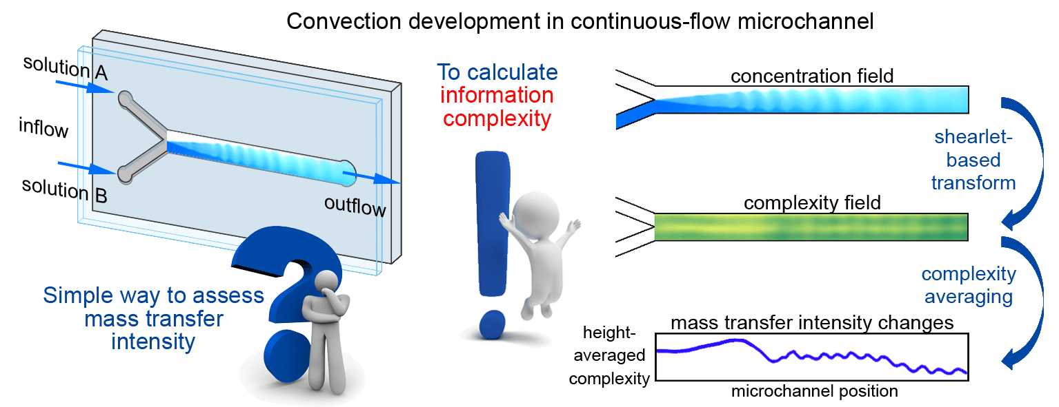
Continuous-flow microchannels are widely employed for synthesizing various materials, including nanoparticles, polymers, and metal-organic frameworks (MOFs), to name a few. Microsystem technology allows precise control over reaction parameters, resulting in purer, more uniform, and structurally stable products due to more effective mass transfer manipulation. However, continuous-flow synthesis processes may be accompanied by the emergence of spatial convective structures initiating convective flows. On the one hand, convection can accelerate reactions by intensifying mass transfer. On the other hand, it may lead to non-uniformity in the final product or defects, especially in MOF microcrystal synthesis. The ability to distinguish regions of convective and diffusive mass transfer may be the key to performing higher-quality reactions and obtaining purer products. In this study, we investigate, for the first time, the possibility of using the information complexity measure as a criterion for assessing the intensity of mass transfer in microchannels, considering both spatial and temporal non-uniformities of liquid’s distributions resulting from convection formation. We calculate the complexity using shearlet transform based on a local approach. In contrast to existing methods for calculating complexity, the shearlet transform based approach provides a more detailed representation of local heterogeneities. Our analysis involves experimental images illustrating the mixing process of two non-reactive liquids in a Y-type continuous-flow microchannel under conditions of double-diffusive convection formation. The obtained complexity fields characterize the mixing process and structure formation, revealing variations in mass transfer intensity along the microchannel. We compare the results with cases of liquid mixing via a pure diffusive mechanism. Upon analysis, it was revealed that the complexity measure exhibits sensitivity to variations in the type of mass transfer, establishing its feasibility as an indirect criterion for assessing mass transfer intensity. The method presented can extend beyond flow analysis, finding application in the controlling of microstructures of various materials (porosity, for instance) or surface defects in metals, optical systems and other materials that hold significant relevance in materials science and engineering.Graphic Abstract
Keywords
Microfluidic continuous-flow technologies are actively employed for synthesizing new substances and materials in modern research and technology. The small channel dimensions allow precise control of reaction parameters and mass transfer, thereby enhancing the efficiency of the synthesis process. Continuous-flow technology allows for precise control of size, shape, and porosity in synthesized substances, making it crucial for fields such as catalysis, medicine, and materials science. In these processes, convection plays a critical role, significantly impacting mass transfer and reactant mixing along the channel. Forced convection is generated either randomly, for instance, through pump operation, or intentionally to intensify the mixing process, as it happens in channels with complex external and internal geometries [1]. Natural convection may arise due to local changes in concentration and temperature, giving rise to buoyancy-driven convection [2] or changes in surface tension, initiating Marangoni convection [3].
On the one hand, convection positively affects the synthesis process by enhancing reactant mixing and reaction progression. On the other hand, local convection may lead to uneven substance distribution, affecting the internal structure of the reaction product. In the case of synthesizing crystalline materials (e.g., metal-organic structures [4]), it can result in external defects, diminishing their quality and functional characteristics. Thus, the investigation of convective flows in microfluidic systems is a pivotal factor in ensuring the high efficiency of flow synthesis.
The most common methods for visualizing and investigating flows and pattern formation in microchannels utilize dilution-based methods [5]. These methods include introducing a dye into one of the streams, enabling the assessment of mutual liquid mixing. The dilution-based method is known for its simplicity, affordability, and widespread accessibility, making it an economical and straightforward approach that requires minimal resources, and thus widely adopted by researchers. Various criteria are utilized to analyze the spatial distribution of the dye, including the mixing degree (terms such as mixing intensity or mixing efficiency are also mentioned in the literature and denote the same criterion) [6], criteria based on Lagrangian analysis [7] and Shannon entropy index [8,9]. The dependence of any aforementioned criteria on the channel length reflects dye distribution uniformity, enabling conclusions about the quality of flow mixing. However, to optimize the mixing process, it is also essential to control the development of convective structures and the variation in mass transfer intensity in local channel regions and across the entire system.
Conventional methods for detecting local flow heterogeneities and pattern formation in microchannels typically involve the analysis of fluid velocity distributions using techniques like micro-PIV [10,11] or the assessment of fluid concentration fields through confocal microscopy [12,13]. In this study, we investigate the potential of an alternative criterion that applicable to images, obtained by dilution-based methods. We propose employing a statistical measure of information complexity [14–16]. This measure is calculated based on the Shannon entropy value, functioning as a quantitative indicator of the system’s organization and order. The criterion demonstrates high sensitivity, enabling the detection of even subtle color changes in photographs obtained through standard imaging techniques while employing dilution-based methods for visualization. Using the complexity measure can effectively unveil local color inhomogeneities caused by changes in mass transfer intensity, eliminating the need for expensive and complex methods such as micro-PIV and confocal microscopy. This approach not only advances our understanding of the fundamental processes but also enhances the accessibility of the proposed methodology to a broader research audience.
This study explores the potential use of information complexity as a criterion for assessing mass transfer intensity in microchannels, taking into account spatial and temporal inhomogeneities resulting from structure formation and flow. We calculate complexity and entropy measures for experimental images that demonstrate the mixing of two liquids in a horizontal microchannel under conditions of double-diffusive convection [17]. To compute the Shannon entropy required for complexity calculation, we employ shearlet transform [18]. Applying this transform to the experimental image allows us to generate a two-dimensional entropy field, preserving information about local inhomogeneities and structures. This sets our approach apart from previous studies [19,20], where the mathematical algorithm only permits obtaining an averaged entropy value of Shannon entropy. We investigate entropy and complexity fields for four different mixing scenarios, analyzing two different cases of diffusive mixing: (i) in the absence of fluid flow in the channel (volume flow rate is
2.1 Experimental Setup and Methods
The experiments were conducted in a horizontal Y-shaped microchannel with a rectangular cross-section. The channel dimensions were as follows: length
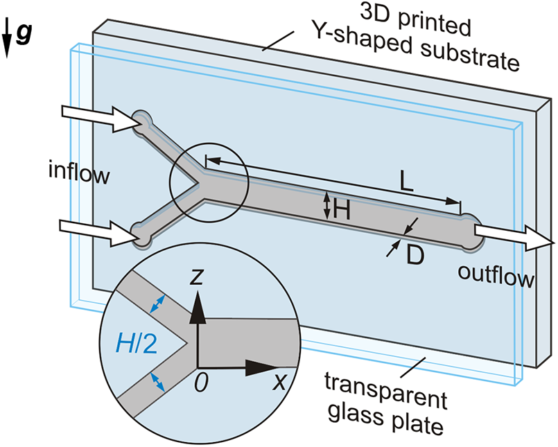
Figure 1: Sketch of the Y-shaped microchannel used
Both arms of the Y-type micro-mixer are connected to an infusion pump (SpLab02) to deliver the working liquids at a consistent flow rate q. The instrumental uncertainty in flow rate, as specified in the manufacturer’s documentation, is ≤± 0.5%. The flow rate within the channel, determined by our geometry, is
We used the pump to create a two-layer fluid-fluid system with a thin horizontal diffusive zone between the layers. The working liquids were introduced along the channel at a flow rate of
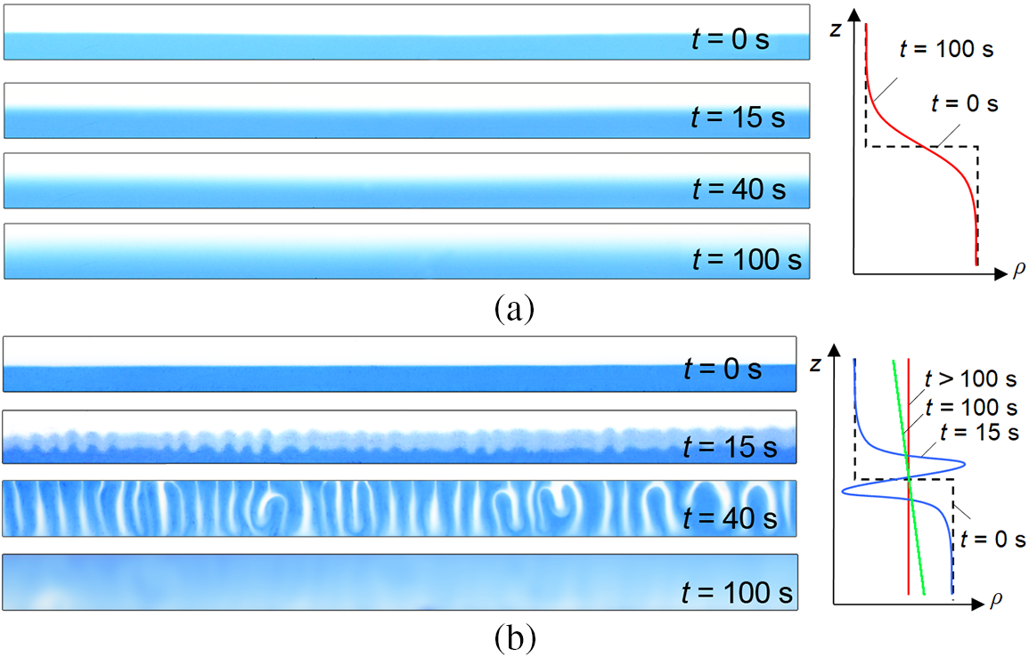
Figure 2: Series of images that demonstrate the temporal evolution of the two-layer miscible system in (a) diffusive mixing scenario between water (upper layer) and water solution of NaOH (lower layer) and (b) convective mixing scenario between water solutions of Na2SO4 (upper layer) and NaOH (lower layer) in the case
For the investigation of the non-stationary case (
2.2 Experiments in the Q = 0 Case
In the first two series of experiments (i and iii), we investigated the process of liquid mixing under zero flow conditions. Fig. 2 presents two sets of images illustrating the evolution of a two-layer system of mixing liquids under pure diffusive mixing conditions (Fig. 2a) and in the presence of double-diffusive convection (Fig. 2b). In the absence of flow, the structure of both two-layer systems is nearly uniform along the channel length. Consequently, we cropped the images to showcase only the central part of the channel, ensuring better visibility of the structure of the fluid. The right side of each figure schematically depicts the time evolution of the length-averaged vertical profile of the general density. The solution for the time-dependent base-state density profile was obtained through a linear stability analysis based on a quasi-steady-state approximation in [21]. We emphasize, that we did not derive these density profiles from experimental measurements but rather depict them schematically, according to the authors’ results [21].
In the case of diffusive mixing (Fig. 2a), at the
Let us briefly describe the mechanism of convection formation. The phenomenon of double diffusion occurs in multi-component stably stratified miscible systems, where the density of the liquid medium is controlled by two (or more) components, at least one of which is distributed unstably and has a molecular diffusion rate different from the other components [21,22]. In the Na2SO4-NaOH system, both components contribute to the stratification of the system with the same sign, meaning an increase in the concentration of any substance leads to an increase in the solution’s density. Therefore, in this configuration, the vertical distribution of the component dissolved in the upper layer (Na2SO4) is unstable [23]. Since the molecular diffusion rate of the stably distributed component (NaOH) is greater than that of the unstably distributed one, double-diffusive convection (or “salt fingering”) develops in the system [24]. For more information on types and mechanisms of double-diffusive instability formation, refer to the monograph [23].
As a result of the development of instability, finger-like structures form in the mixing zone. Convective fingers spread symmetrically up and down, passing through each other, facilitating the rapid mixing of the diffusive zone between the initial liquids. A qualitative analysis of the images shows that after 100 s, the distribution of the dye inside the channel is almost uniform, indicating homogeneity in its concentration. However, it is worth noting that there are still areas in the channel where the dye distribution is uneven. Comparing image series obtained for convective and diffusive mixing mechanisms without flow confirms that convection significantly accelerates the homogenization process of the system but may create regions with non-uniform concentrations.
2.3 Experiments in the Q ≠ 0 Case
Fig. 3 provides visual representations of the flow structure within the channel under continuous-flow conditions. Diffusive and convective mixing scenarios are displayed in Figs. 3a and 3b, respectively. Additionally, schematic profiles in Fig. 3 demonstrate variations in the vertical density distribution along the channel.
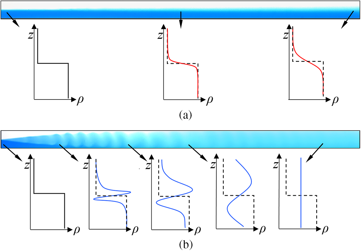
Figure 3: Visualization of the flow structure during diffusive (upper image) and convective (lower image) mixing mechanisms. The plots in the figure illustrate the local density profile
Each image captured under continuous-flow conditions simultaneously showcases all the successive stages of the dynamics of the two-layer miscible system depicted in the image series obtained under zero-flow conditions (Fig. 2). In essence, this flow visualization acts as a comprehensive space-time map, characterizing the evolution of the mixing process. In a diffusive mixing, the liquids near the Y-junction are also initially separated by a thin diffusive zone. As the liquids progress downstream, the diffusive zone gradually expands in the transverse direction. The density profile undergoes a blurring effect along the z-axis, maintaining its nearly step-like nature and a monotonic character. It is worth noting that the channel length is insufficient for complete liquid mixing. In the case of convective mixing, the flow structure drastically changes. The diffusive zone widens rapidly at the Y-junction, indicating a change in the mass transfer mechanism due to the onset of double-diffusive instability. The instability initiates the formation of distinct finger-like structures, persisting prominently from the channel entrance up to its midpoint. Subsequently, these convective fingers gradually dissipate, signifying a diminishing convective intensity. Ultimately, the convective structure vanishes entirely, leaving the distribution of color dye almost uniform in height, indicating the high uniformity of the pumped mixture.
The mechanism of convection decay becomes clearer when analyzing the evolution of the density profile of the system. The unstable density gradients, arising from the development of double-diffusive instability, gradually diminish over time due to the mixing in the diffusive zone between the flows. The intensive mixing takes place due to the unique structure of double-diffusive convection. Convective fingers propagate symmetrically upward and downward, crossing each other, ultimately pushing the mixing process. This process equalizes the concentrations of substances dissolved in the layers, contributing to the reduction of unstable density gradients and the intensity of convection. For a more in-depth understanding of the dynamics of double-diffusive instability in continuous-flow microchannels, refer to [25].
Unlike diffusive mixing, where the mass transfer type remains consistent throughout the entire channel length, the convective mixing scenario exhibits a dynamic evolution of the mass transfer mechanism. Near the Y-junction, convection dominates as the primary mass transfer mechanism. However, as we move toward the end of the channel, a transition occurs, and the prevailing mechanism gradually shifts to diffusion. Determining the dominant mass transfer type in areas with pronounced convective structures is relatively straightforward. However, in regions where the structure is less distinct (e.g., near the Y-junction or in the central part of the channel in Fig. 3b), establishing the prevailing mass transfer type only through visual analysis is challenging. Furthermore, the occurrence of convective mass transfer does not always lead to the formation of structures, and not all visualization methods may detect it even when they are present. For example, finger structures were not observable during the visualization of the development of double-diffusive convection employing Rhodamine B fluoron dye [26]. To distinguish between convective and diffusive mixing scenarios in the channel, it is essential to establish a criterion that aids experimenters in determining the spatial characteristics of mass transfer within the studied system. As such a criterion, we propose using the entropy measure of information complexity [14,16,20,27], which is calculated from experimentally obtained images. If local structural formation occurs during continuous-flow synthesis, the analysis of complexity value can reveal spatial changes and the associated mass transfer type.
3 Entropy and Complexity Measures
The term “information Shannon entropy” is a fundamental concept in information theory and was introduced by Claude Shannon in 1949 [28]. This criterion measures the degree of uncertainty in an information system. The general expression of the Shannon entropy is determined by the probabilities p from:
where N represents the total number of outcomes i, and p is the probability of outcome i occurring.
To simplify the analysis, researcher often use the normalized Shannon entropy value
where S[p] denotes Shannon entropy applied to a specific probability distribution p.
The normalization factor Smax assumes equiprobable distributions for all states and is determined as:
Thus, the entropy of the analyzed distribution p is calculated by the sum with opposite signs of all relative frequencies of the occurrences of states with index i, multiplied by their binary logarithms [10].
Entropy serves as a measure of the inherent disorder within the original signal and exhibits two extreme values. When
The calculation of the entropy value (see Eqs. (1)–(3)) requires constructing the probability distribution of its states. Each pixel in the digital image represents a distinct state characterized by its color value. The probability distribution for color values is then constructed, enabling the assessment of uncertainty in the image structure. For a binary black-and-white image, the number of possible states
In the scientific literature, there are two prevalent entropy concepts: permutation entropy, typically computed using the Bandt-Pompe algorithm [15,20], and spectral entropy [16,27]. While permutation entropy is commonly employed for analyzing one-dimensional data sequences, it also finds applications in digital image analysis [20]. However, the characteristics of the Bandt-Pompe algorithm provide only an average probability distribution, making it unsuitable, since we need to detect local inhomogeneities. Spectral entropy delves into the frequency domain of a signal, evaluating its structural composition and energy distribution across frequencies. This evaluation can be accomplished using the Fourier transform, the wavelet transform, or the shearlet transform. The latter, a subtype of the wavelet transform, distinguishes itself by its ability to adapt to local directions and structures in data, proving particularly effective for analyzing anisotropic signals. Both entropy concepts present advantages over the classical method of constructing probability distributions by tallying the frequency of states in a system. Given that each pixel in an image signifies a distinct state of the system, represented by its color value, it necessitates the computation of a probability distribution for each pixel. Hence, an approach based on the shearlet transform becomes preferable. The concept of local spectral entropy was initially formulated mathematically in [30], and only recently has found application in the dynamic processes analysis [16]. The author analyzed the spatial structure of developing astrocytes by the shearlet transform and obtained a map within the “entropy-complexity” parameter space that classifies various stages of astrocyte growth. Also, a classification of structures of invasive carcinoma was derived using the same parameters plane [27].
The author’s approach [16] assumes the transformation of the entropy measure into a spatially distributed field. The analysis of this field enables the identification of which parts of the investigated structure act as sources of order and which generate noise. The liquid mixing scenarios investigated in this study involve spatial-temporal changes (flow structure, shape and characteristic size). These changes in diffusive and convective mixing scenarios develop gradually, starting from the interface between the two liquids. Consequently, the global formulation of entropy gives rise to challenges in differentiating and interpreting the obtained disorder measures. The local formulation of spectral entropy proposed in [16] effectively addresses this issue.
Using the fast finite shearlet transform [18], and following the approach proposed in [16], we investigate two-dimensional structures represented by the image
where E is the energy of shearlet coefficients and is defined as:
In Eq. (5),
The required local version of the probability distribution,
where
where X and Z are the dimensions of the smoothing area. It is essential to emphasize, that we calculate the probability for absolutely all pixels in the image. In this context, the number of system states N is equal to the total number of pixel colors of the analyzed image.
In our study, the local formulation of the probability distribution (6) becomes more relevant compared to the conventional formulation (4). The reason is that spatial changes occurring during the mixing of liquid streams exhibit a local nature. This becomes particularly evident in experiments performed under continuous-flow conditions, where the shape and size of the convective structures undergo considerable spatial variations. With the provided formulas, Eq. (2) takes the following form:
where S[pe] is the entropy of the equiprobable distribution
Let us introduce one more statistical measure, specifically information complexity, which is determined as follows [14,16,31,32]:
In this expression,
After calculating the spectral entropy (8) and the complexity (10) for the image, crucial insights into the system’s characteristics emerge from its plots on the “entropy-complexity” parameter plane [14,15,27]. On this parameter plane, there are two asymptotic scenarios. The first corresponds to an organized, spatially periodic structure with a distinct temporal or spatial scale. In such a case, the system exhibits low entropy and complexity levels (
Before computing the entropy and complexity measures, all images underwent preprocessing. Experimental images include a parasitic signal caused by uneven illumination. To address this, we subtracted the parasitic component from the image to minimize errors. To achieve this, we captured an illuminated channel filled with transparent solutions without dye, obtaining a “reference” image that contains information about background non-uniformity. In RGB mode, each pixel in the digital images has three color values, complicating the algorithm’s computation. To prioritize the algorithm’s focus on convective structures rather than the color noise structure, we converted all color images, including the reference images, to grayscale with an 8-bit color depth. Subsequently, we subtracted the reference image from each subsequent capture and cropped it to the standardized size of
4.1 Analysis of Flow Structure Evolution in the Q = 0 Case
Fig. 4 presents two series of images illustrating the evolution of the system’s complexity field during diffusive (Fig. 4a) and convective (Fig. 4b) mixing. The complexity fields were computed for the images shown in Fig. 2.
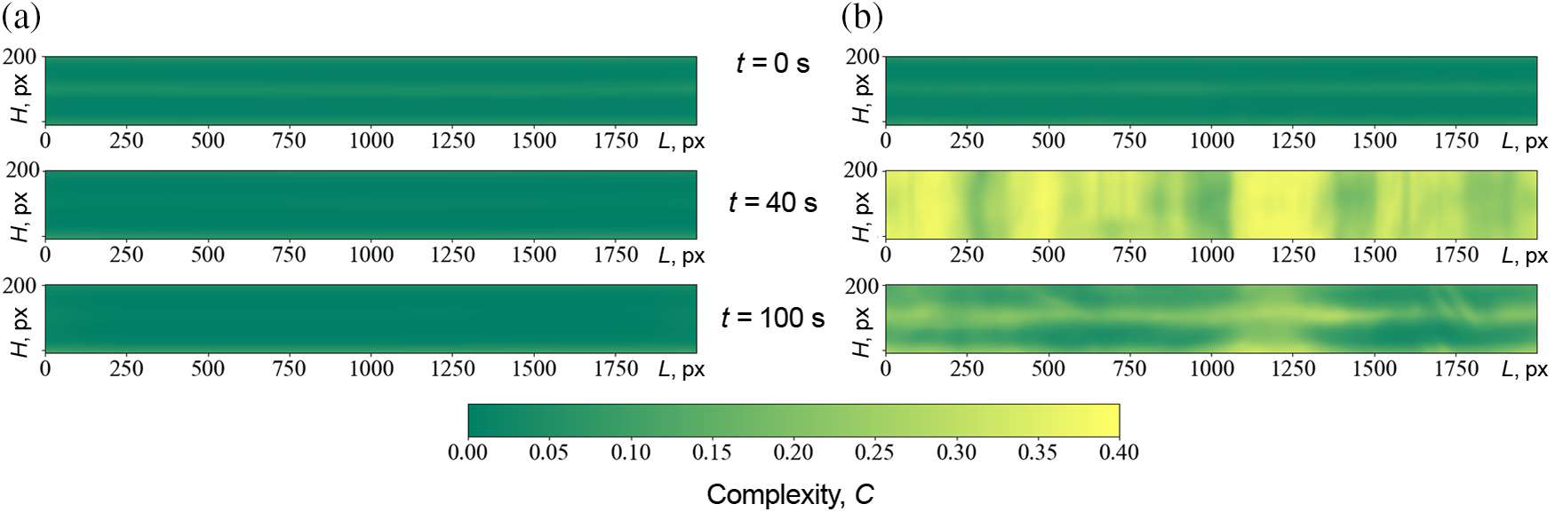
Figure 4: Series of images illustrating the evolution of the complexity field during (a) diffusive and (b) convective mixing of a two-layer liquid system in the absence of pumping
At the initial time (
Subsequently, due to the mutual diffusion process, the vertical size of the mixing zone increases. In the case of diffusive mixing, the zone continues to expand but maintains stability throughout the experiment. Pure diffusive mixing does not lead to qualitative changes in the system, so the complexity, from the perspective of a multiscale structure, remains close to zero throughout the evolution of the mixing process. In the case of convective mixing, the diffusive zone loses its stability due to the development of double-diffusive convection. It results in a significant intensification of layer mixing and a sharp increase in complexity values, indicating a disturbance of the system’s equilibrium [14]. In specific areas of the channel (see
Fig. 5 illustrates the temporal evolution of the height-averaged complexity
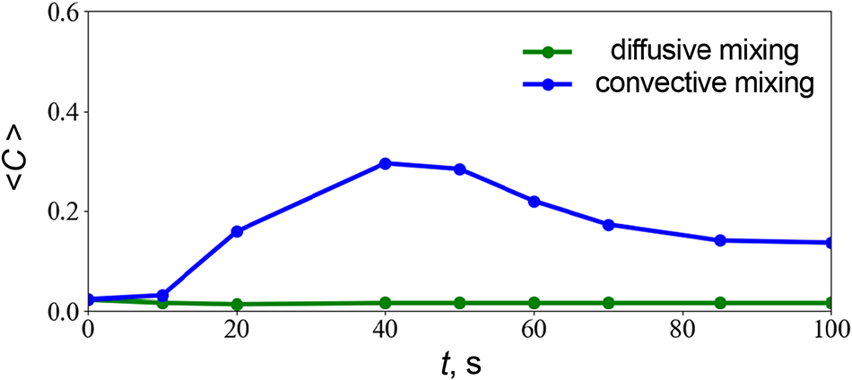
Figure 5: Temporal evolution of the height-averaged complexity value
Looking ahead, we plan to conduct more extensive experimental investigations where both mixing scenarios lead to a new system state (with complete homogeneity) to verify this assumption. Thus, the analysis of the results confirms that the complexity values indeed detect variations in mass transfer type and flow intensity under different mixing scenarios in the absence of flow.
4.2 Analysis of Flow Structure Evolution in the Q ≠ 0 Case
Fig. 6a presents two sets of images illustrating the evolution of the complexity field during diffusive (upper image in Fig. 6a) and convective (lower image in Fig. 6b) mixing under continuous-flow conditions. The complexity fields correspond to the images presented in Fig. 3. Fig. 6b shows the dependence of the height-averaged complexity on the channel length. In diffusive mixing along the channel, there are minimal changes. The flow hinders the transverse mixing of liquids due to the prevalence of its characteristic velocity to the characteristic diffusion rate. As a result, the system state along the channel changes slightly. An exception is the area near the Y-junction, for which the complexity value is maximum. Similar to the stationary case, this is explained by a high initial gradient caused by the presence of a thin diffusive mixing zone between the layers. Further along the channel, this gradient decreases. It brings the system closer to a new equilibrium state and leads to a decrease in the complexity value.
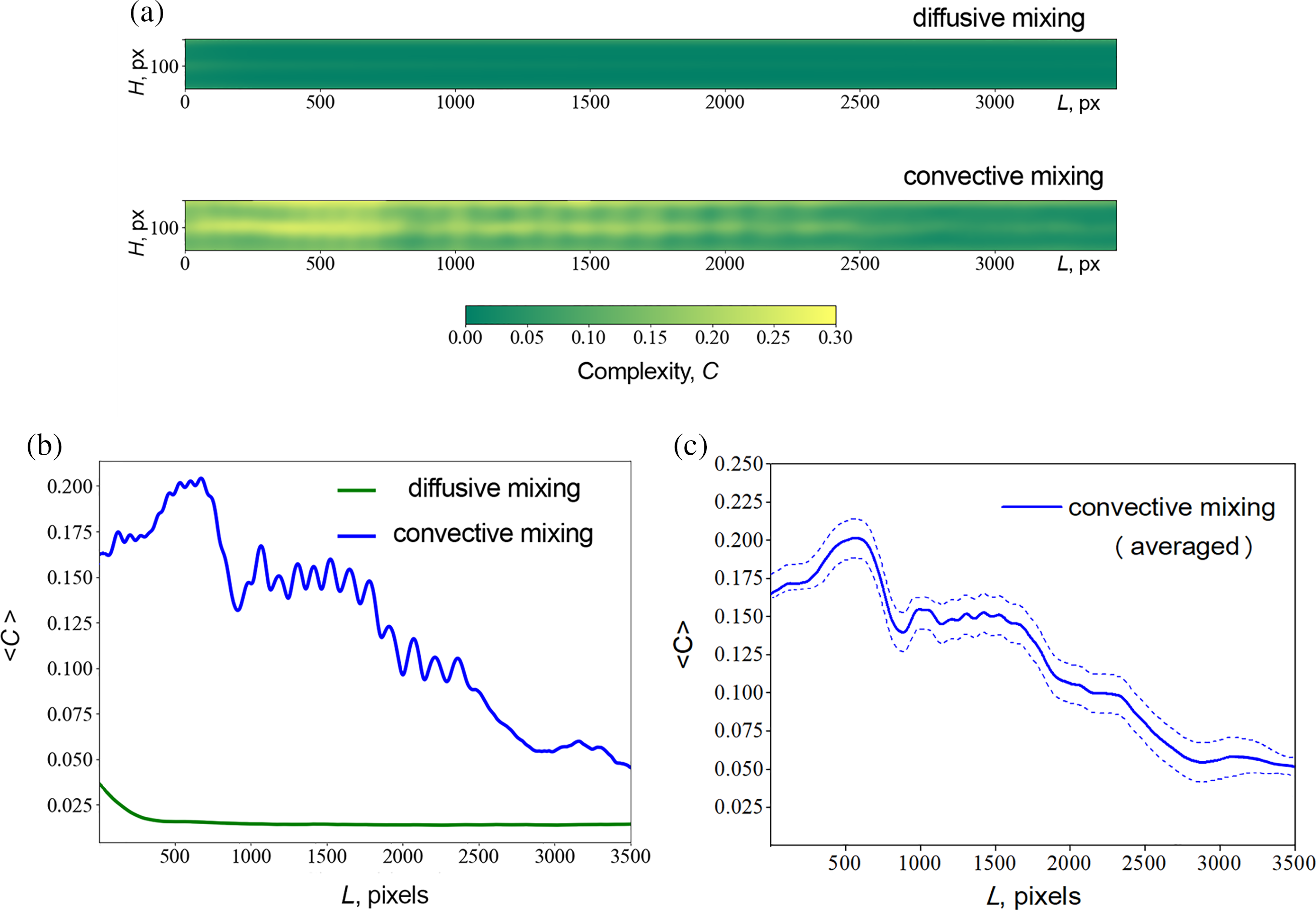
Figure 6: (a) Complexity fields calculated for diffusive (top) and convective mixing (bottom) scenarios of a two-layer liquid system under continuous-flow conditions. (b) Dependence of height-averaged complexity on channel length. (c) The averaged dependence of the height-averaged complexity on channel length. The dashed lines indicate the deviation of
In the case of convective mixing, the obtained complexity field reflects all stages of the convective structure evolution observed in stationary conditions, as described in Section 4.1. The maximum value of the complexity measure is obtained for the initial section of the microchannel, where convective fingers occupy the entire channel height. The complexity-length dependence
The flow irregularities and concentration inhomogeneities can impact the quality and uniformity of the material synthesized in a continuous-flow regime. These irregularities may result from factors such as turbulence, improper temperature control, or uneven distribution of reactants caused by convection. The possibility to detect and visualize irregularities helps prevent defects and optimize synthesis efficiency. Conventional methods for assessing flow patterns in microchannels involve techniques like micro-PIV for velocity analysis or confocal microscopy for concentration fields. In this study, we offer to use an alternative criterion applicable to images obtained by widespread dilution-based methods.
We study the mass transfer dynamics during the mixing process of a two-layer miscible system within a horizontal Y-shaped microchannel. Our investigation encompassed two distinct mixing scenarios: diffusive and convective. In the first case, we examined the trivial diffusive mixing scenario. In the second case, we investigate the intensification of mixing by the double-diffusive instability. We analyzed both scenarios under two conditions: the stationary case (
Obtained complexity fields allowed us to identify the local areas with transition points from diffusive to convective mass transfer, significant for understanding the dynamic of the investigated systems. Also, to illustrate the transition in the type of mass transfer within the channel, we constructed a dependence illustrating changes in the height-averaged complexity measure as a function of channel length. Obtained dependence demonstrated a robust correlation between local convective structure formation and mass transfer intensity. We revealed that the maximal complexity value aligned precisely with the stage of fully formed double-diffusive fingers. It represents the “most complex” (from an information point of view) state with a high mass transfer intensity. As the system became more homogeneous, complexity values decreased, indicating a decrease in mass transfer intensity. This result highlights the efficiency of using complexity measures to detect variations in mass transfer. Despite the advantages of this criterion, there are also drawbacks. Using this criterion imposes stringent requirements on the quality of processed images and, namely, on the pixel noise level. If the useful signal and the parasitic noise are of the same magnitude, the resulting outcome may lack meaningful information. Also, the algorithm presented in this study is suitable for processing grayscale images. In the future, there are intentions to refine the algorithm to analyze RGB images.
In conclusion, our findings confirm that the proposed information complexity measure can indirectly assess mass transfer intensity in liquid media under a continuous-flow regime and in cases without flow. Additionally, the two-dimensional complexity fields provide general information about structure formation and also enable the identification of local inhomogeneities characterizing the uneven distribution of substances dissolved in the system. The results indicate potential applications in optics for detecting local irregularities of optical systems, and in solid mechanics for identifying cracks and defects in solid materials. However, the most extensive prospects lie in microfluidics. Assessing the complexity measure can be beneficial for optimizing microchannel design, improving mixing efficiency, controlling irregularities in reagent distribution, and mitigating disruptions to internal structures and external deformations (such as porosity) in the synthesized substances.
Acknowledgement: The authors have no specific acknowledgement.
Funding Statement: The work was supported by the Ministry of Science and High Education of Russia (Theme No. 368 121031700169-1 of ICMM UrB RAS).
Author Contributions: The authors confirm their contribution to the paper as follows: study conception and design: E. Mosheva; experimental data collection: E. Mosheva; theoretical data collection: I. Krasnyakov; analysis and interpretation of results: E. Mosheva, I. Krasnyakov; writing–original draft preparation: E. Mosheva, I. Krasnyakov; writing–review and editing: E. Mosheva, I. Krasnyakov. All authors reviewed the results and approved the final version of the manuscript.
Availability of Data and Materials: The data that support the findings of this study are available from the corresponding author.
Conflicts of Interest: The authors declare that they have no conflicts of interest to report regarding the present study.
References
1. Dash B, Nanda J, Rout SK. The role of microchannel geometry selection on heat transfer enhancement in heat sinks: a review. Heat Transf. 2022;51:1406–24. [Google Scholar]
2. Soboleva EB. Onset of Rayleigh-Taylor convection in a porous medium. Fluid Dynamics. 2021;56:200–10. [Google Scholar]
3. Kazemi MA, Saber S, Elliott JA, Nobes DS. Marangoni convection in an evaporating water droplet. Int J Heat Mass Transf. 2021;181:122042. [Google Scholar]
4. Koryakina IG, Bachinin SV, Gerasimova EN, Timofeeva MV, Shipilovskikh SA, Bukatin AS, et al. Microfluidic synthesis of metal-organic framework crystals with surface defects for enhanced molecular loading. Chem Eng J. 2023;452:139450. [Google Scholar]
5. Aubin J, Ferrando M, Jiricny V. Current methods for characterising mixing and flow in microchannels. Chem Eng Sci. 2010;65(6):2065–93. [Google Scholar]
6. Heshmatnezhad F, Solaimany Nazar AR. On-chip controlled synthesis of polycaprolactone nanoparticles using continuous-flow microfluidic devices. J Flow Chem. 2020;10:533–43. [Google Scholar]
7. Ma X, Tang Z, Jiang N. Eulerian and Lagrangian analysis of coherent structures in separated shear flow by time-resolved particle image velocimetry. Phys Fluids. 2020;32(6):65101. [Google Scholar]
8. Camesasca M, Manas-Zloczower I, Kaufman M. Entropic characterization of mixing in microchannels. J Micromech Microeng. 2005;15(11):2038. [Google Scholar]
9. Kihara T, Obata H, Hirano H. Quantitative visualization of fluid mixing in slug flow for arbitrary wall-shaped microchannel using Shannon entropy. Chem Eng Sci. 2019;200:225–35. [Google Scholar]
10. Ringkai H, Tamrin KF, Sheikh NA, Mohamaddan S. Evolution of water-in-oil droplets in T-junction microchannel by micro-PIV. Appl Sci. 2021;11(11):5289. [Google Scholar]
11. Silva G, Semiao V, Reis N. Rotating microchannel flow velocity measurements using the stationary micro-PIV technique with application to lab-on-a-CD devices. Flow Meas Instrum. 2019;67:153–65. [Google Scholar]
12. Luo Y, Yang J, Zheng X, Wang J, Tu X, Che Z, et al. Three-dimensional visualization and analysis of flowing droplets in microchannels using real-time quantitative phase microscopy. Lab Chip. 2021;21(1):75–82. [Google Scholar] [PubMed]
13. Mukherjee P, Wang X, Zhou J, Papautsky I. Single stream inertial focusing in low aspect-ratio triangular microchannels. Lab Chip. 2019;19(1):147–57. [Google Scholar]
14. Lopez-Ruiz R, Mancini YL, Calbet X. A statistical measure of complexity. Phys Lett A. 1995;209:321–6. [Google Scholar]
15. Bandt C, Pompe B. Permutation entropy: a natural complexity measure for time series. Phys Rev Lett. 2002;88(8):174102. [Google Scholar] [PubMed]
16. Brazhe A. Shearlet-based measures of entropy and complexity for two-dimensional patterns. Phys Rev E. 2018;97:61301. [Google Scholar]
17. Turner JS. Double-diffusive phenomena. Annu Rev Fluid Mech. 1974;6(1):37–54. [Google Scholar]
18. Hauser S, Steidl G. Fast finite shearlet transform. Available from: https://arxiv.org/abs/1202.1773. [Accessed 2014]. [Google Scholar]
19. Fodor PS, Itomlenskis M, Kaufman M. Assessment of mixing in passive microchannels with fractal surface patterning. EPJ App Phys. 2009;47(3):31301. [Google Scholar]
20. Zunino L, Ribeiro HV. Discriminating image textures with the multiscale two-dimensional complexity-entropy causality plane. Chaos Solitons Fractals. 2016;91:679–88. [Google Scholar]
21. Trevelyan PMJ, Almarcha C, de Wit A. Buoyancy-driven instabilities of miscible two-layer stratifications in porous media and Hele-Shaw cells. J Fluid Mech. 2011;670:38–65. [Google Scholar]
22. Gershuni GZ, Zhukhovitsky EM. On the convectional instability of a two-component mixture in a gravity field. J App Math Mech. 1963;27(2):441–52. [Google Scholar]
23. Radko T. Double-diffusive convection. London: Cambridge University Press; 2013. [Google Scholar]
24. Kumar S, Gangawane KM, Oztop HF. Applications of lattice Boltzmann method for double-diffusive convection in the cavity: a review. J Therm Anal Calorim. 2022;147(20):10889–921. [Google Scholar]
25. Bratsun DA, Siraev RR, Pismen LM, Mosheva EA, Shmyrov AV, Mizev AI. Mixing enhancement by gravity-dependent convection in a Y-shaped continuous-flow microreactor. Microgravity Sci Technol. 2022;34(5):90. [Google Scholar]
26. Mizev AI, Mosheva EA, Shmyrov AV. Double-diffusive convection in the continuous flow microreactors. J Phys Conf Ser. 2021;1945(1):012036. [Google Scholar]
27. Bratsun DA, Krasnyakov IV. Study of architectural forms of invasive carcinoma based on the measurement of pattern complexity. Math Model Nat Phenom. 2022;17:15. [Google Scholar]
28. Shannon CE. A mathematical theory of communication. Bell Syst Tech J. 1949;27(3):379–423. [Google Scholar]
29. Alemaskin K, Manas-Zloczower I, Kaufman M. Entropic analysis of color homogeneity. Polym Eng Sci. 2005;45(7):1031–8. [Google Scholar]
30. Powell GE, Percival IC. A spectral entropy method for distinguishing regular and irregular motion of Hamiltonian systems. J Phys A Math Gen. 1979;12:2053–71. [Google Scholar]
31. Ribeiro HV, Zunino L, Lenzi EK, Santoro PA, Mendes RS. Complexity-entropy causality plane as a complexity measure for two-dimensional patterns. PLoS One. 2012;7:e40689. [Google Scholar] [PubMed]
32. Sethna JP. Statistical mechanics: entropy, order parameters, and complexity. USA: Oxford University Press; 2021. [Google Scholar]
33. Dagan I, Lee L, Pereira F. Similarity-based methods for word sense disambiguation. In: Proceedings of the 35th Annual Meeting of the Association for Computational Linguistics and 8th Conference of the European Chapter of the Association for Computational Linguistics, 1997; Madrid, Spain. p. 56–63. [Google Scholar]
34. Schutze H. Foundations of statistical natural language processing. Massachusetts: MIT Press; 1999. [Google Scholar]
35. Prigozhin I. Order out of chaos: a new dialogue between man and nature (In Russian). Moscow: Progress Publishers; 1986. [Google Scholar]
36. Kolmogorov AN. Local structure of turbulence in an incompressible fluid at very high Reynolds numbers. Proc USSR Acad Sci. 1941;30(4):299–303. [Google Scholar]
Cite This Article
 Copyright © 2024 The Author(s). Published by Tech Science Press.
This work is licensed under a Creative Commons Attribution 4.0 International License , which permits unrestricted use, distribution, and reproduction in any medium, provided the original work is properly cited.
 Downloads
 Citation Tools