
 Submit a Paper
 Propose a Special lssue
 Open Access
ARTICLE

A New Device for Gas-Liquid Flow Measurements Relying on Forced Annular Flow
1 Petroleum Engineering Technology Research Institute, SINOPEC Shengli Oilfield Company, Dongying, 257000, China
2 School of Petroleum Engineering, Yangtze University, Wuhan, 430100, China
* Corresponding Author: Xingkai Zhang. Email:
Fluid Dynamics & Materials Processing 2024, 20(8), 1759-1772. https://doi.org/10.32604/fdmp.2024.049035
Received 25 December 2023; Accepted 27 February 2024; Issue published 06 August 2024
 View Full Text
 Download PDF
Abstract
A new measurement device, consisting of swirling blades and capsule-shaped throttling elements, is proposed in this study to eliminate typical measurement errors caused by complex flow patterns in gas-liquid flow. The swirling blades are used to transform the complex flow pattern into a forced annular flow. Drawing on the research of existing blockage flow meters and also exploiting the single-phase flow measurement theory, a formula is introduced to measure the phase-separated flow of gas and liquid. The formula requires the pressure ratio, Lockhart-Martinelli number (L-M number), and the gas phase Froude number. The unknown parameters appearing in the formula are fitted through numerical simulation using computational fluid dynamics (CFD), which involves a comprehensive analysis of the flow field inside the device from multiple perspectives, and takes into account the influence of pressure fluctuations. Finally, the measurement model is validated through an experimental error analysis. The results demonstrate that the measurement error can be maintained within ±8% for various flow patterns, including stratified flow, bubble flow, and wave flow.Keywords
Nomenclature
| Frg | Froude number |
| Pr | Pressure difference ratio |
| ρ | Fluid density (kg/m3) |
| β | Equivalent diameter ratio |
Differential pressure flow meters [1–3], which are indispensable instruments in modern industrial production and daily life, play a crucial role in fields such as petrochemicals, heating, and water supply. There are also many researches on differential pressure flowmeters. For example, Zheng et al. [4] studied the metering characteristics of the long-throat venturi tube, Lisowski et al. [5] studied the characteristics of differential pressure flowmeter under wet steam, Liu et al. [6] designed a new type of dual differential pressure dynamic flowmeter, and Amirante et al. [7] studied the measurement of supercritical carbon dioxide flow by Venturi flowmeter. A blocking flow meter [8–10] is a type of differential pressure flow meter that employs alternating expansions and contractions within the pipeline to induce a certain level of acceleration and deceleration in the fluid. Due to the pressure difference generated during the process, a stable differential pressure signal is produced before and after the narrowest section of the throttle. This differential pressure is directly proportional to the fluid velocity. Therefore, the fluid flow rate can be determined by monitoring the changes in the differential pressure signal.
Borkar et al. [11] conducted tests on a bi-directional cone flowmeter under fully developed flow conditions and evaluated its performance under double 90° bends. The results showed that the bi-directional cone flowmeter was insensitive to the vortices generated by double 5° bends placed upstream of the cone flowmeter when the distance was 90.9 times the diameter (D) or greater. Feng et al. [12] proposed a new type of differential pressure flowmeter with an olive-shaped flowmeter (OSF) and studied it through experiments and numerical analysis. Flow lines, pressure, and velocity were obtained and numerically analyzed. The results showed that the pressure in the OSF was more stable, ensuring high measurement accuracy and repeatability. The OSF outperformed the original pressure flowmeter (OPF) in terms of relative pressure loss, flow line distribution, pressure distribution, and velocity distribution. Singh et al. [13] experimentally evaluated the performance characteristics of a V-cone flowmeter with different diameter ratios, taking into consideration the Reynolds number and upstream disturbance. The experiments were conducted using water and oil to cover a wide range of Reynolds numbers. The effect of the upstream velocity profile was investigated by placing a gate valve upstream of the V-cone flowmeter at various distances and conducting experiments under different valve opening conditions. RK Singh et al. [14] used FLUENT in their study to investigate the influence of cone apex angle and upstream vortices on the performance of the cone flowmeter. The calculation results of the flow coefficient values showed that, in the presence of upstream disturbances in the form of vortices, the flow coefficient values were also independent of Reynolds number and slightly influenced by the size of the vortices. Flow within the longitudinal plane indicated the presence of a pair of counter-rotating vortices in the downstream recirculation region.
Existing research on obstructive flowmeters has established various flow measurement models by analyzing the relationship between pressure differential signals and fluid flow rates. However, the measurement accuracy is inevitably affected by complex flow patterns. In order to eliminate the errors caused by complex flow patterns in gas-liquid flow measurement, this paper proposes a gas-liquid flow measurement device consisting of swirl blades and a capsule-shaped throttle. The swirl blades are used to transform the complex flow patterns into a forced circular flow, which can to some extent avoid the influence of complex flow patterns. This has significant implications for major industrial sectors such as petrochemicals and process control, especially in reducing errors in fossil fuel measurement, which can minimize fuel waste and reduce carbon emissions.
Next, we will combine CFD simulations and fluid experiments to establish a flow measurement model for the capsule-shaped throttle flowmeter under forced circular flow conditions.
2 Numerical Computation Method
The VOF (Volume of Fluid) model has been chosen as the multiphase flow model in this study. The VOF model is based on the assumption that two or more fluids do not interpenetrate each other. For each phase in the gas-liquid two-phase flow, the variable “phase” is used to represent the volume fraction in each computational cell. The sum of the volume fractions of the two phases in each control cell is equal to 1. Based on the volume fraction values, the variables in any given cell represent either one phase or a mixture of the gas-liquid two phases.
In the VOF model, the immiscible fluids of the gas-liquid two phases share a set of momentum equations, and the volume fraction of each phase is tracked in each computational cell throughout the flow domain. The governing equations for mass and momentum of unsteady free flow can be expressed as follows.
2.1.1 The Equation of Continuity
The continuity equation for solving the volume fraction of the gas-liquid two phases is given by the following expression:
where mpq and mqp represent the mass transfer from gas phase to liquid phase and from liquid phase to gas phase, respectively. Sαq denotes the source term. The volume fraction equation for the primary phase is not solved directly as it is computed based on the following relationship:
The VOF equation can be solved using implicit or explicit time discretization.
A single momentum equation is solved throughout the entire flow field, with the resulting velocity field shared among the different phases. The momentum equation depends on the volume fractions of all phases in q and l.
The equation can be transformed into Reynolds-averaged Navier-Stokes (RANS) equations:
where p represents pressure, g is the gravitational acceleration, U is the mean velocity, and i and j are integers from 1 to 3.
In this study, the turbulence model adopts the Reynolds Stress Model, which has demonstrated good applicability in solving conditions involving swirling flows, vortex flows, and more.
2.3 Solution Methods and Boundary Conditions
In this study, the combination of the pressure field and velocity field is processed via the PISO [15] algorithm, with a second-order upwind spatial numerical format and a fixed time discretization method. The initial boundary conditions were set as velocity inlet and pressure outlet.The standard wall function without slip is adopted for the wall surface, and the pressure based solution method for ideal gas is used.
3 Primary Structure of the Measurement Device
The main structure and dimensions of the measurement instrument are depicted in Fig. 1. The vortex blades and capsule-shaped throttle element are mounted concentrically inside the pipeline, with the throttle located 2D downstream of the vortex blades. Three pressure measurement stations [16] are located within the measurement section: one 1D upstream of the throttle, another at the minimum flow area of the throttle zone, and the third 1D downstream of the throttle.
Figure 1: Structure of the measurement device
In the diagram, the inner diameter (D) of the pipeline is 40 mm. The height (h) and width (w) of the vortex blades are 20 and 15 mm, respectively, with a thickness (δ) of 1 mm. The blades have a swirled angle (α) of 60°. The throttle has a diameter (d) of 10 mm and a length (l) of 30 mm.
4 Grid Partition and Irrelevance Verification
Using the ANSYS ICEM module, the measurement equipment was structured grid partitioned [17]. Fig. 2 shows the grid partitioning results, which indicate an average cell grid quality of 0.85 and a minimum orthogonal quality of 0.6, indicating a positive grid quality.
Figure 2: Grid partitioning results
The grid density is crucial for the accuracy of flow field calculations. The fewer the number of grids, the lower the simulation precision [18]; however, excessively dense grids increase computation time and place higher demands on computer performance. Therefore, it is necessary to conduct grid independence verification. During the grid independence verification process, 7 sets of grids were analyzed, with grid quantities of 106 × 104, 124 × 104, 139 × 104, 154 × 104, 165 × 104, 187 × 104, and 226 × 104, respectively. The pressure difference (P1-P2) was obtained for each grid quantity, as shown in Fig. 3. It can be observed that there is no significant change in the calculation results of each flow pattern when the grid quantity increases from 185 × 104 to 259 × 104, but the computational efficiency decreases. Therefore, to achieve an appropriate balance between accuracy and computational efficiency, this study selects a grid quantity of 165 × 104.
Figure 3: Grid independence verification
5 Principles and Models of Measurement
The study presented a two-phase flow measuring system which utilizes a spinning blade placed ahead of the throttler as a means to transform the intricate and unstable gas-liquid flow pattern into a forced circular flow. This method enabled the development of a measurement model for gas-liquid two-phase flow, reducing the impact of flow pattern on measurement and improving flow measurement accuracy and stability. Fig. 4 depicts a schematic depiction of the forced circular flow.
Figure 4: Schematic diagram of forced annular flow
Based on the Bernoulli equation and the continuity equation, the mass flow rate of single-phase flow can be represented in the following form:
In the equation, Mdg represents the mass flow rate of single-phase flow; ε denotes the expansion coefficient of the fluid; C is the discharge coefficient; β represents the equivalent diameter ratio of the measurement device; ΔPtp stands for the pressure difference inside the pipe; ρg represents the density of the single phase; and A denotes the cross-sectional area of the pipe. Among them:
The mass flow rate of the gas phase in the gas-liquid two-phase mixture can be obtained by introducing a virtual head correction factor φ.
The mass fraction of the gas phase in the gas-liquid two-phase mixture can be expressed in the following form:
In the equation, Ml represents the mass flow rate of the liquid phase; ρl is the density of the liquid phase; ρg is the density of the gas phase; XLM is the L-M number (Lockhart-Martinelli number), which is a dimensionless quantity.
Therefore, the mass flow rate of the gas phase in the two-phase mixture can be expressed in the following form:
To obtain the L-M number (XLM) and the correction factor (φ), the pressure difference ratio (Pr) and the gas phase Froude number (Frg) are introduced. The relationship between Pr, Frg, XLM, and φ can be determined through fitting or regression analysis.
In the equation, ΔPf is the pressure difference between the upstream pressure (P1) and the pressure at the throat of the throttle valve (P2); ΔPb represents the pressure difference between the downstream pressure (P3) and (P2); D denotes the pipe inner diameter; Usg is the gas phase superficial velocity; and g stands for the acceleration due to gravity.
It is apparent that a fitting calculation is required to obtain the complete expression for the gas phase mass flow rate. Therefore, experimental data is necessary to establish relationships between the different parameters, and Matlab will be utilized to fit and determine the values of their respective coefficients.
6 Validation of Numerical Simulation Reliability
6.1 Experimental Setup and Experimental Procedure
The experimental setup and associated equipment can be observed in Figs. 5 and 6. In the course of the experiment, an appropriate volume of water is initially introduced into the water storage tank. Subsequently, the water is pumped from the tank to the gas-liquid mixing tank via a water pump, while the gas is conveyed to the mixing tank through an air compressor. Within the mixing tank, a gas pipeline is connected to a bubble generator positioned beneath the liquid surface. Following agitation, a significant number of bubbles are generated within the mixing tank and evenly dispersed throughout the liquid. The blended fluid is then transferred to the horizontal experimental pipe section, and at the end of the experimental section, a reflux pump is used to recycle the experimental water. In the experiment involving the measurement of gas-liquid two-phase flow rate using a forced annular flow capsule flowmeter, all parameters are continuously recorded using digital data acquisition software.
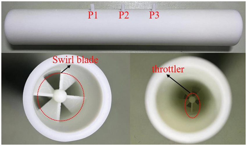
Figure 5: Experimental model diagram
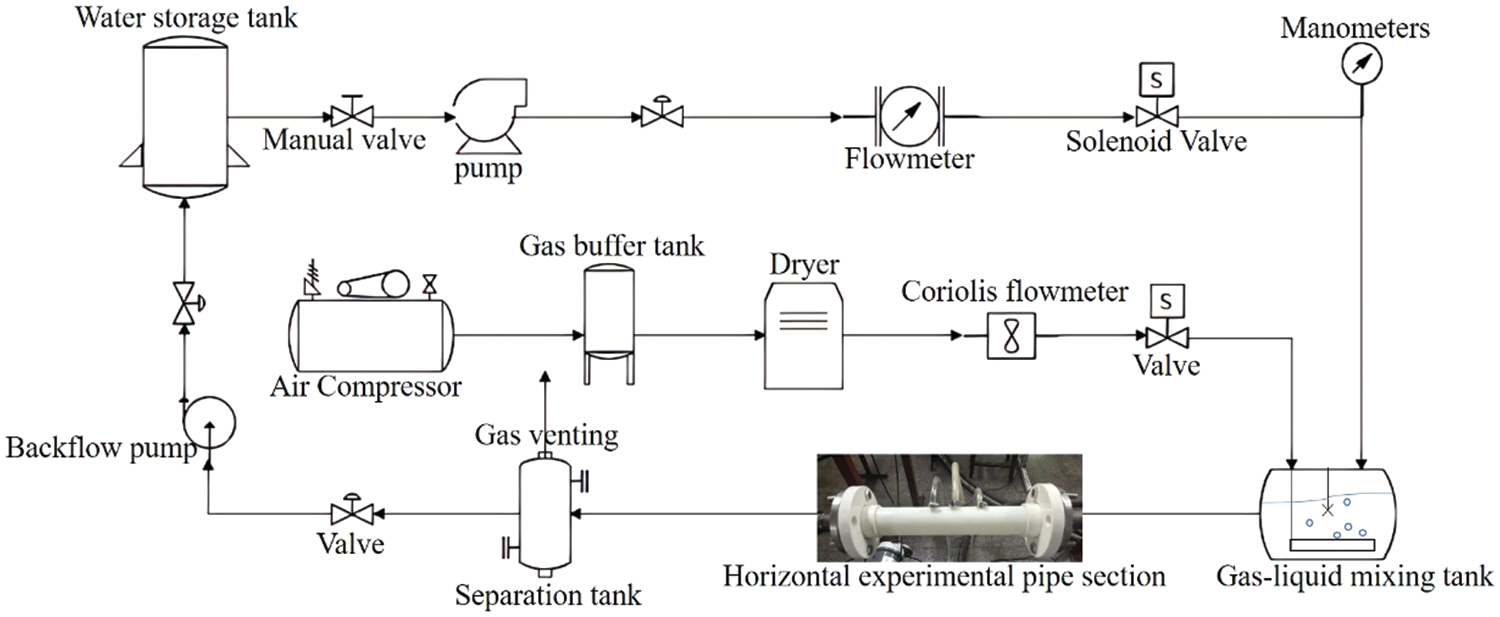
Figure 6: Experimental process diagram
6.2 Comparison between Experiment and Simulation
To verify the reliability of the numerical simulation, we randomly set up nine groups of gas phase flow rates and liquid holdups for both the numerical simulation and fluid experiments. The working medium for both the experiment and simulation is air and water, and they are conducted at room temperature and atmospheric pressure. The following Fig. 7 compares the pressure ratio (Pr) of three pressure measurement points in the experiment and simulation. It can be seen that the experimental results are consistent with the simulation results, indicating the numerical simulation has a certain level of reliability.
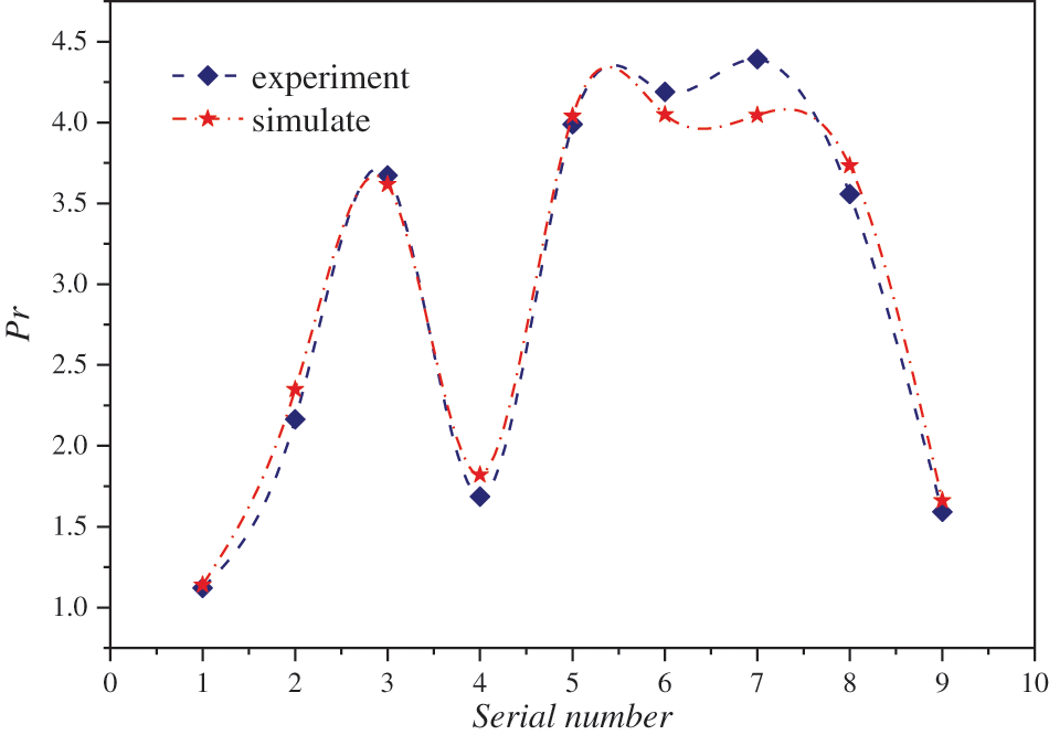
Figure 7: Experimental and simulation comparison
Observing the dynamic distribution of the flow field within a measurement device is essential for studying variations in the flow field, selecting pressure measurement points, and processing measurement parameters [19]. Using an inlet velocity of 10 m/s and a liquid holdup of 0.2 as an example, the following maps depict the liquid phase distribution, velocity cloud, and Q-criterion iso-surface inside the measurement device. To enhance the visual representation of the flow field in the device, five cross-sections were uniformly selected before and after the swirl vanes and throttling device.
Based on the analysis of Figs. 8 and 9, it can be observed that as the gas-liquid mixture passes through the swirl vanes, the velocity significantly increases due to the reduction in the flow area. Additionally, the swirling effect of the vanes causes the two-phase flow to gradually separate, with denser liquid being thrown towards the wall surface while less dense gas moves towards the center. This results in the formation of a ring-shaped flow in the form of a gas core-liquid film.

Figure 8: Liquid phase distribution
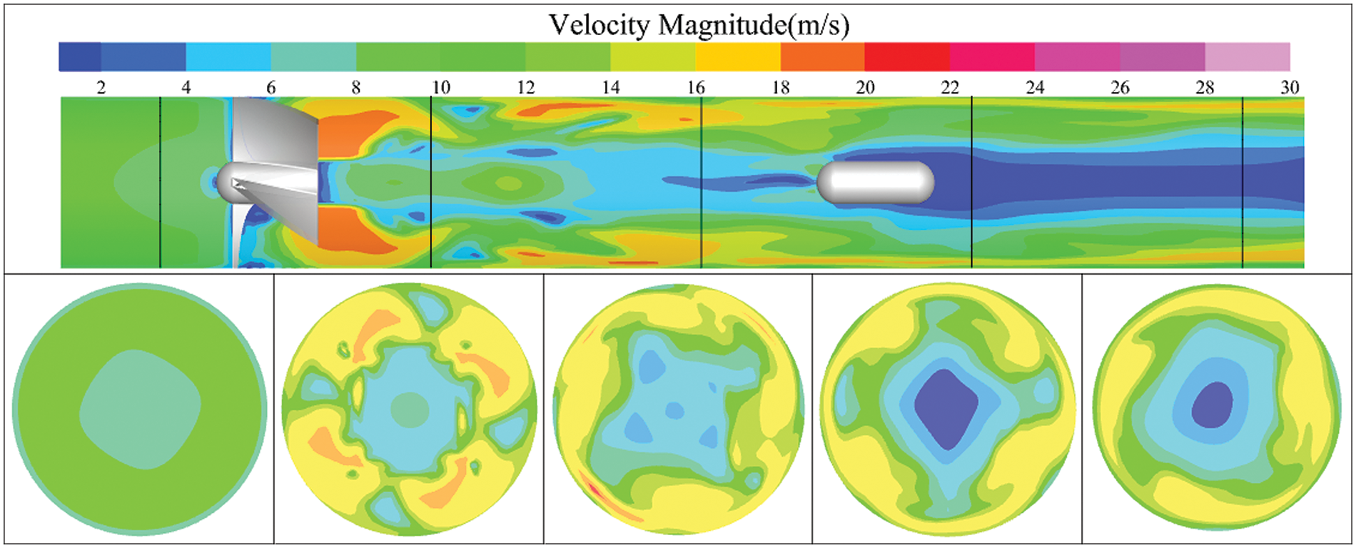
Figure 9: Velocity contour map
Fig. 10 shows the iso-surface map based on the Q-criterion, which reveals the generation of numerous vortices within the device. The region between the swirl vanes and the throttling device forms a central vortex, while multiple spiral arms behind the swirl vanes create external vortices. Moreover, the interaction between the central vortex and the external vortices gives rise to local vortices in the front section of the throttling device. The external and central vortices play a crucial role in maintaining the fluid’s annular flow, whereas local vortices may exacerbate pressure fluctuations near the throttle, leading to measurement instability at pressure measurement point. Therefore, appropriately processing the pressure data at the measurement points is important to mitigate the impact of pressure fluctuations [20].
Figure 10: Iso-surface map of Q-criterion
7.2 Processing of Pressure Data
The pressure values measured at the upstream and downstream pressure points of the throttling device display periodic pressure fluctuations due to the disturbance caused by local eddy currents [21]. Taking an inlet velocity of 5 m/s and a liquid holdup of 0.1 as an example, Fig. 11 illustrates the pressure variations at three pressure measurement points, namely P1, P2, and P3, over a specific time interval. From the graph, it can be observed that P1 exhibits the highest pressure value, while P2 has the lowest pressure value due to its smaller flow area. Additionally, the downstream pressure P3 is slightly lower than P1 due to pressure losses caused by wall friction. Furthermore, all three measurement points experience periodic pressure variations over time. To enhance measurement accuracy, the final pressure value is determined by taking the average value of three cycles.
Figure 11: Pressure variation curve
7.3 Determining the L-M Number
The graph in Fig. 12 shows the variation of pressure difference ratio (Pr) with respect to the L-M number. It can be observed that as the L-M number increases, the pressure difference ratio gradually increases. The relationship between the L-M number (XLM) and the pressure difference ratio (Pr) is nonlinear, and the rate of change decreases over time. Furthermore, looking at the vertical axis, it can be seen that as the gas-phase Froude number (Frg) increases, the pressure ratio also increases gradually.
Figure 12: Variation of pressure difference ratio (Pr) with L-M number (XLM) at different froude numbers
Method of obtaining data points in the graph: A gas-phase Froude number (Frg) is selected, which corresponds to a gas-phase superficial velocity. The liquid holdup is then varied from 0 to 1, and the data for three pressure measurement points, along with corresponding values of gas-liquid superficial velocity and liquid holdup, are exported through a report. These data points are calculated using Eqs. (10), (14), and (15).
The obtained data is then fitted using nonlinear polynomial regression in MATLAB. The fitting equation is as follows:
In the formula, i = 1.67, j = 4.139, c = 8.521, d = 10.64, e = 16.173, h = −14.86.
7.4 Determining the Coefficient φ
The variation of coefficient φ with respect to the L-M number (XLM) is shown in Fig. 13. It can be observed that as the XLM number increases, the coefficient φ also increases continuously. There is a linear relationship between the XLM number and the coefficient φ. From the vertical perspective, the coefficient φ gradually decreases with increasing density ratio. Additionally, under different density ratios or Froude numbers, the slope of the coefficient φ with respect to the XLM number varies.

Figure 13: Variation of coefficient φ with L-M number (XLM) under different density ratios or froude numbers
The expressions for the slope (a), intercept (b), and coefficient φ are obtained through fitting, as shown in Eqs. (17)–(19).
Using MATLAB numerical analysis software and conducting numerical calculations, the undetermined parameters of the gas phase mass flow rate prediction formula in gas-liquid two-phase flow have been determined through data processing. To verify the measurement accuracy of the flow rate prediction formula, it will be compared with experimental data obtained from flowmeters.
According to the Mandhane flow pattern map, multiple data points of gas-liquid superficial velocity have been chosen for each flow pattern. These data points are depicted in the Fig. 14 below, which illustrates the observed flow patterns during the experiment.
Figure 14: Mandhane flow pattern map
The relative error between the predicted and actual values of the gas phase mass flow rate under different flow patterns is shown in Fig. 15. It can be observed that the relative errors for each flow pattern are relatively small, mostly within ±8%. Therefore, it is proved that the gas-liquid flow measurement model proposed in this paper has high accuracy and reliable measurement results, and this paper can provide some reference for the research of a differential pressure flowmeter.
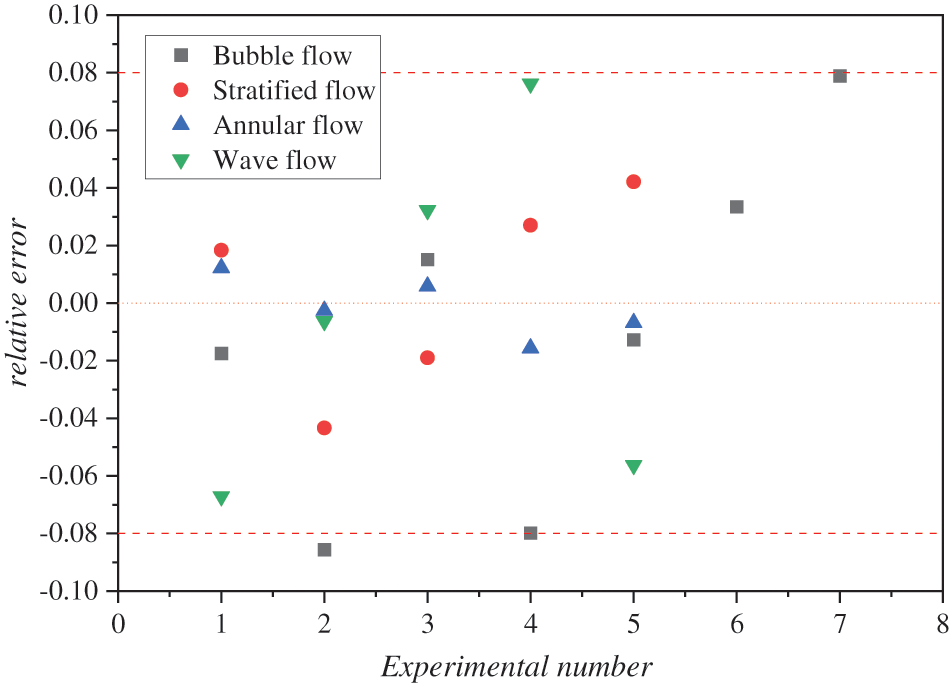
Figure 15: Relative error between predicted and actual values of gas phase mass flow rate under different flow patterns
To mitigate the errors stemming from the intricate flow patterns in gas-liquid flow measurement, a gas-liquid flow measurement apparatus comprising swirl vanes and a capsule throttle has been proposed. This configuration transforms the complex flow pattern into a compelled annular flow pattern by means of the swirl vanes.
Drawing upon single-phase flow measurement principles, a formula for quantifying gas-liquid two-phase flow during compelled annular flow has been developed. This formula combines parameters such as pressure difference ratio, L-M number, and gas phase Froude number. The unknown parameters in this flow measurement equation have been calibrated through CFD numerical simulations. The CFD simulation process encompassed a thorough analysis of the device’s flow field from multiple perspectives, while considering the impact of pressure fluctuations.
In conclusion, an error analysis of the measurement model was conducted in conjunction with fluid experiments. The results demonstrated that across various flow patterns such as stratified flow, bubble flow, and bubbly flow, the measurement errors remained within a range of ±8%. These errors underscore the consistency of the measurements. This study provides valuable insights for advancing gas-liquid flow measurement research.
Acknowledgement: None.
Funding Statement: The authors would like to acknowledge the Supported By Open Fund of Hubei Key Laboratory of Oil and Gas Drilling and Production Engineering (Yangtze University), YQZC202309.
Author Contributions: The authors confirm contribution to the paper as follows: study conception and design: Xingkai Zhang, Tiantian Yu, Hao Zhong; data collection: Tiantian Yu, Hao Zhong, Youping Lv; analysis and interpretation of results: Tiantian Yu, Ming Liu; draft manuscript preparation: Tiantian Yu, Pingyuan Gai, Zeju Jiang, Peng Zhang. All authors reviewed the results and approved the final version of the manuscript.
Availability of Data and Materials: The authors acknowledge the importance of data accessibility in scientific research and strive to promote transparency and reproducibility. In this study, all data were obtained experimentally and presented in the form of data graphs in the article. However, it must be noted that there may be certain instances where data cannot be released due to legitimate reasons. These reasons may include legal or ethical restrictions, privacy concerns, intellectual property rights, or agreements with third parties. We assure you that any unavailability of data is not intended to hinder scientific progress but rather to ensure compliance with applicable regulations and protect the rights and privacy of individuals or entities involved. We thank our readers for their understanding and support in promoting open science while respecting the limitations and constraints associated with data accessibility. Should there be any concerns or inquiries regarding data availability, please feel free to contact us directly.
Conflicts of Interest: The authors declare that they have no conflicts of interest to report regarding the present study.
References
1. Mubarok MH, Cater JE, Zarrouk SJ. Comparative CFD modelling of pressure differential flow meters for measuring two-phase geothermal fluid flow. Geotherm. 2020;86:101801. [Google Scholar]
2. Dehkordi PB, Colombo LPM, Guilizzoni M, Sotgia G. CFD simulation with experimental validation of oil-water core-annular flows through Venturi and Nozzle flow meters. J Petrol Sci Eng. 2017;149:540–52. [Google Scholar]
3. Amirante R, Catalano LA, Poloni C, Tamburrano P. Fluid-dynamic design optimization of hydraulic proportional directional valves. Eng Optimiz. 2014;46(10):1295–314. [Google Scholar]
4. Zheng WB, Liang RM, Zhang XK, Liao RQ, Wang D, Huang LM. Wet gas measurements of long-throat Venturi Tube based on forced annular flow. Flow Meas Instrum. 2021;81:102037. [Google Scholar]
5. Lisowski E, Filo G, Rajda J. Pressure compensation using flow forces in a multi-section proportional directional control valve. Energ Convers Manage. 2015;103:1052–64. [Google Scholar]
6. Liu T, Zhibing Z, Zhigang Y. Research on double differential pressure dynamic flowmeter. High Technol Letters. 2019;25(4):8:378–385. [Google Scholar]
7. Amirante R, Distaso E, Tamburrano P. Experimental and numerical analysis of cavitation in hydraulic proportional directional valves. Energ Convers Manage. 2014;87:208–19. [Google Scholar]
8. Liu W, Zhang T, Xu Y, Qi F, Li B. Optimal angle combinations of cone flow meter selection based on viscous stress scale factors. Chinese J Scientific Instrum. 2015;36(7):1497–505. [Google Scholar]
9. He DH, Chen S, Bai BF. Online detection of wet gas-liquid phase flow based on pressure loss ratio of V-cone flowmeter. J Instrum. 2018;39(7):235–44. [Google Scholar]
10. Wang ZH, Zhang XK, Liao RQ, Ma ZX, Wang D, Yang WX. Measurement of high water-cut heavy oil flow based on differential pressure of swirling flow. Phys Fluids. 2024;36(1). [Google Scholar]
11. Borkar K, Venugopal A, Prabhu SV. Study on the design and performance of a bi-directional cone flowmeter. Flow Meas Instrum. 2013;34:151–9. [Google Scholar]
12. Feng GZ, Guo YJ, Shi DC, Gu C, Yu FY, Long TH, et al. Experimental and numerical study of the flow characteristics of a novel olive-shaped flowmeter (OSF). Flow Meas Instrum. 2020;76:101832. [Google Scholar]
13. Singh SN, Seshadri V, Singh RK, Gawhade R. Effect of upstream flow disturbances on the performance characteristics of a V-cone flowmeter. Flow Meas Instrum. 2006;17:291–7. [Google Scholar]
14. Singh RK, Singh SN, Seshadri V. Study on the effect of vertex angle and upstream swirl on the performance characteristics of cone flowmeter using CFD. Flow Meas Instrum. 2009;20:69–74. [Google Scholar]
15. Zhao J, Ning Z, Lv M. Large eddy simulation of the two-phase flow pattern and bubble formation process of a flow mixing nozzle under a gas-liquid mode. Fluid Dyn Res. 2019;51:55510. [Google Scholar]
16. Zhang J, Wang XW, Bai BF, He DH. Online measurement of gas and liquid flow rate in wet gas through one V-cone throttle device. Exp Therm Fluid Sci. 2016;75:129–36. [Google Scholar]
17. Meng J, Liu ZP, An K, Yuan MN. Simulation and optimization of throttle flowmeter with inner-outer tube element. Meas Sci Rev. 2017;17(2):68–75. [Google Scholar]
18. Li X, Xiao XF, Cao L. Excitation condition analysis of guided wave on PFA tubes for ultrasonic flow meter. Ultrasonics. 2016;72:134–42. [Google Scholar]
19. Zhuang Y, Zhang N, Ma L, Huang Y. Numerical investigation of liquid flowmeter calibration device based on CFD. J Physic: Conf Seri. 2018;1071(1). [Google Scholar]
20. Liu WG, Xu Y, Zhang T, Qi FF. Experimental optimization for dual support structures cone flow meters based on cone wake flow field characteristics. Sensor Actuat A-Phys. 2015;232:115–31. [Google Scholar]
21. Zheng DD, Shao SM, Liu AN, Wang MS, Li T. Soft measurement model for wet gas flow rate based on ultrasonic and differential pressure sensing. Meas Sci Technol. 2024;35(5):055003. [Google Scholar]
Cite This Article
 Copyright © 2024 The Author(s). Published by Tech Science Press.
This work is licensed under a Creative Commons Attribution 4.0 International License , which permits unrestricted use, distribution, and reproduction in any medium, provided the original work is properly cited.
 Downloads
 Citation Tools