
 Submit a Paper
 Propose a Special lssue
 Open Access
ARTICLE

Phase Transition in a Dense Swarm of Self-Propelled Bots
Applied Physics Department, Perm National Research Polytechnic University, Perm, 614990, Russia
* Corresponding Author: Dmitry Bratsun. Email:
(This article belongs to the Special Issue: Advanced Problems in Fluid Mechanics)
Fluid Dynamics & Materials Processing 2024, 20(8), 1785-1798. https://doi.org/10.32604/fdmp.2024.048206
Received 30 November 2023; Accepted 01 March 2024; Issue published 06 August 2024
 View Full Text
 Download PDF
Abstract
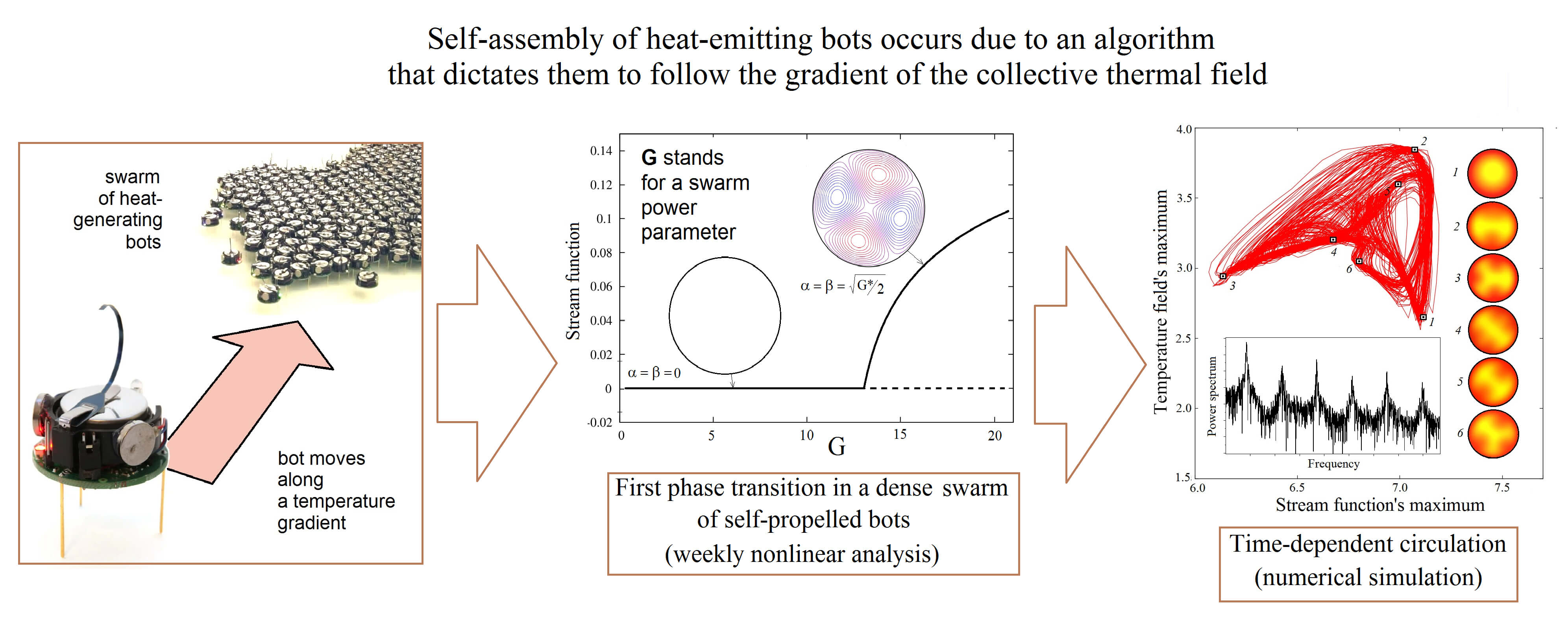
Swarms of self-organizing bots are becoming important elements in various technical systems, which include the control of bacterial cyborgs in biomedical applications, technologies for creating new metamaterials with internal structure, self-assembly processes of complex supramolecular structures in disordered media, etc. In this work, we theoretically study the effect of sudden fluidization of a dense group of bots, each of which is a source of heat and follows a simple algorithm to move in the direction of the gradient of the global temperature field. We show that, under certain conditions, an aggregate of self-propelled bots can fluidize, which leads to a second-order phase transition. The bots’ program, which forces them to search for the temperature field maximum, acts as an effective buoyancy force. As a consequence, one can observe a sudden macroscopic circulation of bots from the edge of the group to its center and back again, which resembles classical Rayleigh-Benard thermal convection. In the continuum approximation, we have developed a mathematical model of the phenomenon, which reduces to the equation of a self-gravitating porous disk saturated with an incompressible fluid that generates heat. We derive governing equations in the Darcy-Boussinesq approximation and formulate a nonlinear boundary value problem. An exact solution to the linearized problem for infinitesimal perturbations of the base state is obtained, and the critical values of the control parameter for the onset of the bot circulation are calculated. Then we apply weakly nonlinear analysis using the method of multiple time scales. We found that as the number of bots increases, the swarm exhibits increasingly complex patterns of circulation.Graphic Abstract
Keywords
Nomenclature
| Symbols | |
| D | Area occupied by bots |
| F | Effective volumetric force |
| G, G0 | Dimensionless parameter of a swarm power and its critical value, respectively |
| g | Coefficient in Eq. (3) |
| Jn | Bessel function of nth order |
| n, l | Azimuthal and radial wave numbers, respectively |
| p | Pressure field |
| Q | Power of heat generated by bots |
| R | Characteristic size of a swarm |
| r, φ | Polar coordinates |
| T | Thermal field |
| T0 | Thermal field in the base state |
| u | Fluid filtration velocity in a porous medium model |
| x, y | Cartesian coordinates |
| Greek Symbols | |
| α, β | Time-dependent amplitudes |
| Γ | Domain boundary |
| ε | Supercriticality parameter |
| θ | Temperature disturbance |
| ν | Kinematic viscosity coefficient |
| ρ0 | Medium density |
| τ | Slow time in amplitude Eq. (27) |
| Φ | Сomplex function in Eq. (14) |
| χ | Thermal diffusivity coefficient |
| ψ | Stream function disturbance |
In recent years, active media have increasingly attracted the attention of researchers. Most often, an active medium is defined as an aggregate of elements capable of independently moving and interacting with each other [1]. The study of such systems provides a deeper understanding of self-assembly processes, in which relatively simple building blocks spontaneously combine into structures with a complex hierarchical architecture [2]. Self-assembly is expected to be a fundamental basis for the development of technologies for the production of new functional materials [3]. Note that the smaller the block, the higher the interest in developing technologies that include natural self-assembly mechanisms.
As is known, each element of the active medium must be able to borrow energy from the external environment and transform it into its movement in space. Although there are examples of self-propelled elements of a purely physical or chemical nature, we primarily mean living objects. As is known, the survival of organisms largely depends on their ability to adapt to environmental changes. Chemotaxis is one of the simplest but most effective adaptation mechanisms [4]. Many microorganisms can detect the concentration of a chemical and move along its gradient. This ability allows bacteria to find nutrients, transmit signals to each other, and plays a crucial role in the emergence of collective behavior for the survival of the entire microbe population [5]. Similar phenomena are observed among cells of a mesenchymal phenotype, such as cancer cells, which can differentiate within a tumor for collective survival [6,7]. Collective cell behavior during tissue growth in the scaffold is also observed [8].
Bioconvection is another well-known example of this kind [9]. This phenomenon is observed in solutions with aerotactic bacteria, whose movement along the oxygen gradient leads the medium to a second-order phase transition, which triggers the macroscopic ordered movement of the elements of the medium. In addition to chemotaxis, the phenomenon of phototaxis is known: some algae search for optimal levels of light intensity for photosynthesis [10]. Sensitivity to light and spatial self-organization is also demonstrated by some fungal organisms [11]. Communication between bacteria to produce the bioconvection can be carried out through various fields. Theoretical models for the instability development due to chemical reactions were developed in [12,13]. The effect of phototaxis, being the propensity of bacteria to move toward a light source, was modeled in [14,15]. Generally, bioconvection develops in inhomogeneous and non-isothermal media [16–18].
Such phenomena among higher animals are much more difficult to differentiate from social behavior in a group, and therefore they have been studied much less well. For example, complex oscillatory movements are observed in birds, fish, and deer [19]. But a simple explanation for these phenomena based on physical mechanisms is not enough here, since the main trigger for such behavior is social adaptation, and not an unconditioned reflex. The wintering behavior of emperor penguins is a remarkable case, as it demonstrates collective behavior based on simple physical principles [20–22]. When the weather worsens in winter, these animals show a sporadic transition to a dense flock consisting of hundreds (sometimes thousands) of individuals. Inside a densely packed crowd, the temperature is sufficient for survival. A number of studies have shown that such a medium can demonstrate not only the self-assembly of individuals, but also phase transitions of the 1st and 2nd order [23].
An artificial object, for example, a bot, which operates according to a certain algorithm, can also be an element of the active environment. The processes of self-assembly and self-organization in the environment of interacting cyborgs or microrobots have been studied in a number of works [24–27]. If in [24,25], the authors study the self-assembly of robots from a theoretical point of view, then the work [26] represented a breakthrough in the field of experiment, as it proposed the design of cheap but functional robots (no more than $10), which could move independently and coordinate collective actions. An even more striking result was presented in [27], where an inexpensive biotechnology for creating self-propelled cyborgs based on externally controlled bacteria was proposed. These works showed that creating a large swarm of bots of one nature or another is already possible in practice. In [28], the effect of excitation of Turing structures was studied in an environment of hundreds of kilobots programmed with a certain simple algorithm for communications between nearest neighbors. Thus, it was shown that a swarm of robots is capable of reproducing reaction-diffusion processes.
In this work, we theoretically study the effect of sudden fluidization of a dense group of bots, which leads to the excitation of their convective flows. Each bot is assumed to be a heat source, equipped with temperature sensors, and follows a simple program to move in the direction of the gradient of the global temperature field. An element of the swarm under consideration could well be the appropriately reprogrammed kilobot proposed in [26]. We have developed a mathematical model of the phenomenon in the continuum approximation and demonstrate some solutions obtained within the model. The work is intended to demonstrate that the laws of behavior of complex systems are the same for systems with elements of different natures.
Let us assume that the swarm consists of identical bots both in functionality and in the underlying algorithm of actions. Let each bot execute the following program. First, it produces heat at a fixed source power Q. Second, it measures the temperature at several points on its periphery and calculates the direction of the global thermal field gradient (thermotaxis). Third, the bot moves in 2-D space in the direction of the gradient (Fig. 1a). The preliminary process of assembling the bots into a dense mass is not considered in this work. We will consider the properties of an already emerged swarm, which can generally occupy an arbitrary, not necessarily simply connected, region D with a characteristic size R (Fig. 1b). For simplicity, we assume that the shape of the region is stationary. In this case, a swarm of bots can be considered as a continuous environment, the elements of which have the ability to move within given boundaries Γ. Depending on the view D, both Cartesian and polar coordinates can be used (Fig. 1b).
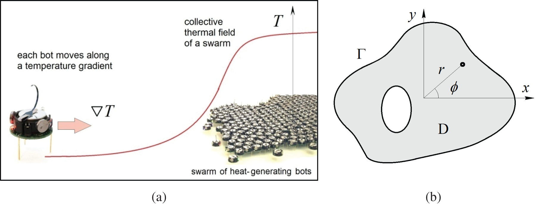
Figure 1: (a) Self-assembly of heat-emitting bots occurs due to an algorithm that dictates them to follow the gradient of the collective thermal field; (b) Schematic representation of a dense swarm of bots occupying domain D with boundary Γ, and a 2-D coordinate system
The global thermal field T (r,φ) is the result of the collective interaction of bots. It also serves as an intermediary for the exchange of information between bots. Let us write the heat conduction equation in the following form:
where u (r,φ)–the velocity of the medium element, ρ0–medium density, χ и cp–the effective coefficients of thermal diffusivity and heat capacity of the swarm, respectively. The right side of Eq. (1) contains terms that affect the change in the temperature field. The first term describes the standard process of heat diffusion. In a dense group of bots, heat is lost due to heat transfer between bots when they are in direct contact. Here, we neglect losses due to heat transfer to the surrounding space, considering the thermal conductivity coefficient of air to be negligible. The second term describes the process of heat generation by bots. We assume that the bots do it in a stationary and uniform manner. Therefore, the heat release per unit area of the swarm is characterized by the constant Q. Finally, the last term on the right side of (1) describes the advection of heat, which occurs due to the movement of bots in space. Generally, Eq. (1) stands for the standard equation for heat transfer in a 2-D medium with internal heat sources [29].
The dense packing of bots determines the inertia-free movement of environmental elements with high internal friction, which is conveniently described by the Darcy equation:
where ν и K–the effective coefficients of viscosity and permeability of the medium, respectively; F–effective volumetric force acting on each swarm element. In fluid mechanics, Eq. (2) is usually used to describe liquid filtration through a porous medium with an extremely low porosity coefficient [30]. However, one can apply such an approach to describe complex systems with individual dynamics if the processes in the system occur in a highly dissipative manner. For example, the movement of cells in tissue occurs without inertia, which requires the use of Aristotelian mechanics [7,8]. In the latter, forces directly determine the velocity of bodies. It is exactly the approach we use in Eq. (2). When bots gather in a dense group, their further movement is not prohibited but becomes difficult. In the model, this requires omitting the time derivative in (2). Nevertheless, system (1), (2) is still non-stationary since changes in the thermal field in Eq. (1) are determined primarily by the effect of thermal conductivity and not by the movement of bots in space. Therefore, the system under consideration is a thermally controlled one: first, the thermal field changes and the velocities of bots then adapts to these changes.
Now we need to set the feedback between the bots’ movement and the thermal field. The main driving force in the system is determined by the desire of the bots to move closer to the maximum temperature value of the global thermal field:
where g is the coefficient of the corresponding dimension (K−1s−2). By substituting (3) into Eq. (2) and redefining the pressure in such a way as to absorb the gradient term, we obtain:
We non-dimensionalize length, time, velocity, pressure, and temperature in Eqs. (1) and (4) using the units R, R2/χ, χ/R, νχρ0/K, and (νQ/2ρ0cpgK)1/2, respectively. This choice of units allows us to reduce the linearized equations for temperature and velocity to a symmetric form. In turn, this simplifies the solution of the stability problem (see below). So, we obtain a system of dimensionless equations that determine the circulation of heat-generating bots in a dense swarm, represented as an incompressible heat-generating fluid filling a self-gravitating porous disk:
Eq. (5) contain the only dimensionless parameter of the problem:
which quadratically depends on the characteristic size of the swarm R. Thus, the parameter G can be interpreted as the power of the swarm. Let us formulate the boundary conditions:
Here, we assume that the temperature at the boundary is maintained constant and equal to Text due to the rapid removal of heat into the surrounding space. Eqs. (5) and (7) represent a boundary value problem for determining the dynamics of bots depending on the power of the swarm G.
A state of mechanical equilibrium in a swarm can be established if two conditions are met. Firstly, the temperature gradient and the direction of the body force must be parallel at all points of the domain under consideration [31]. This condition is always satisfied in our problem due to the assumption about the properties of force (3). Secondly, the shape of region D must be such that the swarm boundary coincides with the isotherm. If this is not the case, then the temperature distribution at the boundary should have a special form, which contradicts the boundary condition (7). The circular shape of the area satisfies both of these requirements.
Let us consider a swarm of a round shape with radius R. In this case, Eqs. (5) and (7) admits a steady state solution that describes the stationary position of the bots. We will refer this state of the system as the base one. Let us set the speed of the bots equal to zero and look for a solution for the temperature field in the form T0(r). Then we get:
By solving problem (8), we obtain:
We can see from (9), that the maximum temperature in a stationary swarm is achieved in the center.
Let us rewrite problem (5)–(7), (9) for finite perturbations near the base state (9):
Substituting (10) into Eqs. (5) and (7) and introducing the stream function in polar coordinates:
we get the following problem:
Let us linearize Eq. (11) near the base state (9):
Eq. (13) have a remarkable property: if a pair of functions (ψ0, θ0) is a solution to problem (12), (13), then the functions (θ0, –ψ0) also satisfy these equations. Thus, all critical values of the parameter G are doubly degenerate.
By introducing the complex function Φ(r,φ) = ψ(r,φ) + iθ(r,φ), we obtain the following problem for determining the eigenvalues of the operator:
We look for a solution to problem (14) in the following form:
where n stands for the azimuthal wavenumber. Substituting (15) into (14), we obtain the problem:
which has the solution:
where Jn is n-th order Bessel function, C stands for the integration constant. Notice that, when deriving solution (17), we used the condition that the solution is bounded at the point r = 0.
The solvability condition for problem (16) requires the equality:
which allows us calculating the spectrum of eigenvalues of the radial operator (16). Let us number the radial part of the solution with the index l. Table 1 shows the critical values of the swarm power parameter G0 for the first five motion modes. The characteristic pattern of circulation of bots in a round swarm, which corresponds to the neutral mode of movement, is also shown in the table.
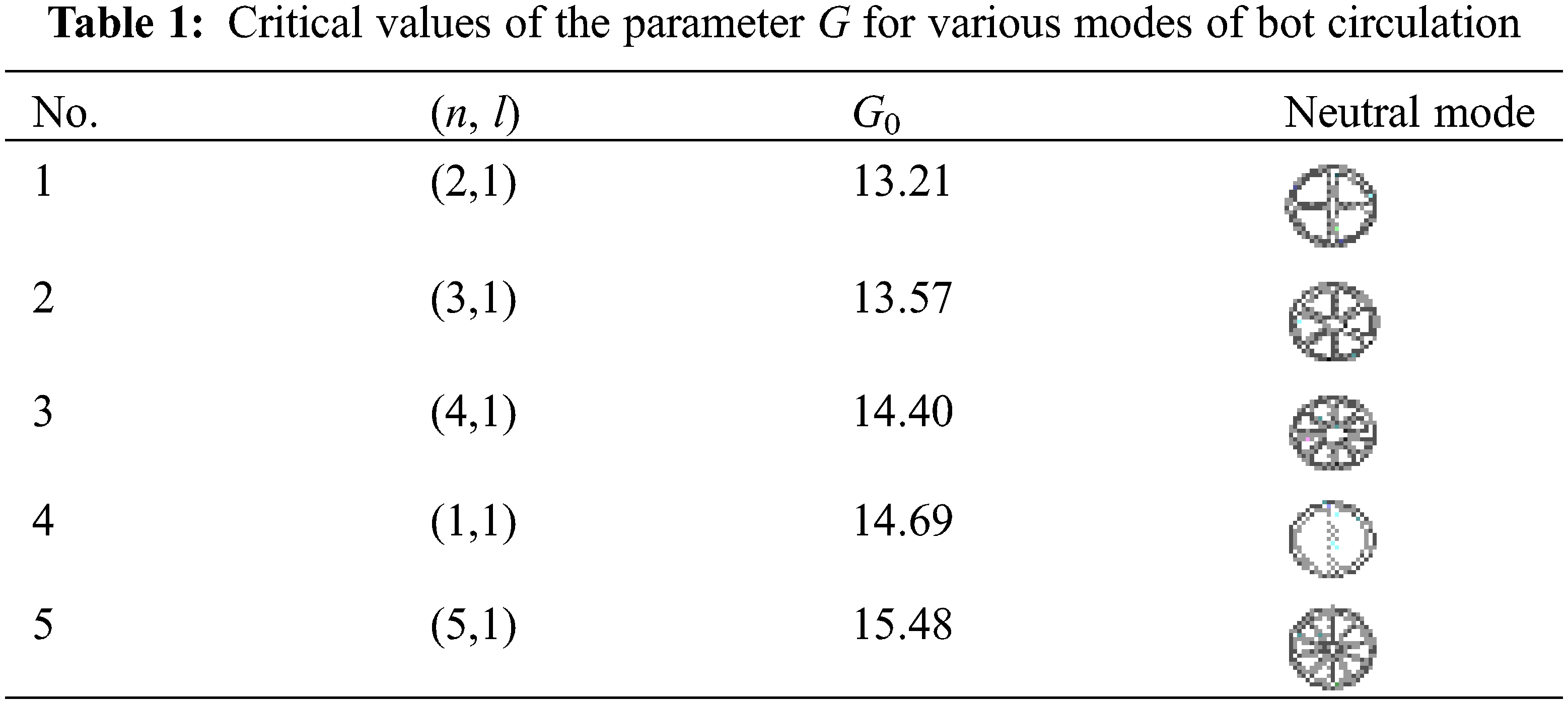
The first mode that loses stability is (2,1)-its crisis occurs at G0 = 13.21. Immediately after it, the (3,1)-mode is excited, then the (4,1)-mode and so on. Fig. 2 shows the perturbations of the stream function (left) and temperature (right) calculated for the most dangerous (2,1)-mode at the bifurcation point G0.
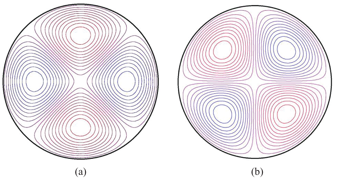
Figure 2: Neutral perturbations of the stream function ψ (a) and temperature θ (b) for the most dangerous (2,1)-mode of movement of bots in a swarm. Red and blue vortices rotate clockwise and counterclockwise, respectively
3.3 Weakly Non-Linear Analysis
In this section, we study the branching of steady-state solutions near the first bifurcation point G0 within the weakly nonlinear theory. To do this, we expand the variables, the parameter G and the differential time operator into series with respect to the small parameter ε:
where ε stands for the supercriticality defined by:
By substituting expansions (19) into Eqs. (11) and (12) and by collecting terms of the same order of the magnitude, we obtain at the leading order:
In the second order we have:
The third-order problem is:
It is easy to see that problem (20) coincides with (12), (13), which we already solved above. In the higher orders (21) and (22), new terms appear on the right-hand sides that perturb problem (20). One can prove that linear operator (20) is self-adjoint [32]. This makes it possible to specify the scalar product of two arbitrary vector functions A: (A1, A2) and B: (В1, В2) in the following form:
and require the solvability of each of the problems (21), (22) in the form of the orthogonality of the right-hand sides with respect to the solution of the leading-order problem (20):
By taking into account the double degeneracy of the spectrum of critical values, we represent the solution to the problem (20) in the following form:
where α and β stands for the amplitudes dependent on slow times.
By requiring the fulfillment of the solvability condition (24) for problem (21), we obtain:
Eq. (26) are linear in amplitudes, therefore G1 = 0, ∂/∂t1 = 0.
By repeating the procedure for problem (22), we obtain the following amplitude equations:
where
Thus, the solution to the problem near the first bifurcation has the form:
Nontrivial steady states of (27) include a one-parameter family:
of monotonically stable attractors existing due to the rotational symmetry of the problem.
Fig. 3a shows the phase portrait of the dynamical system (28) above the first bifurcation point. The variation of the stream function with the growth of the swarm power is shown in Fig. 3b. When G* > 0, the stationary flows of bots are excited in the system.
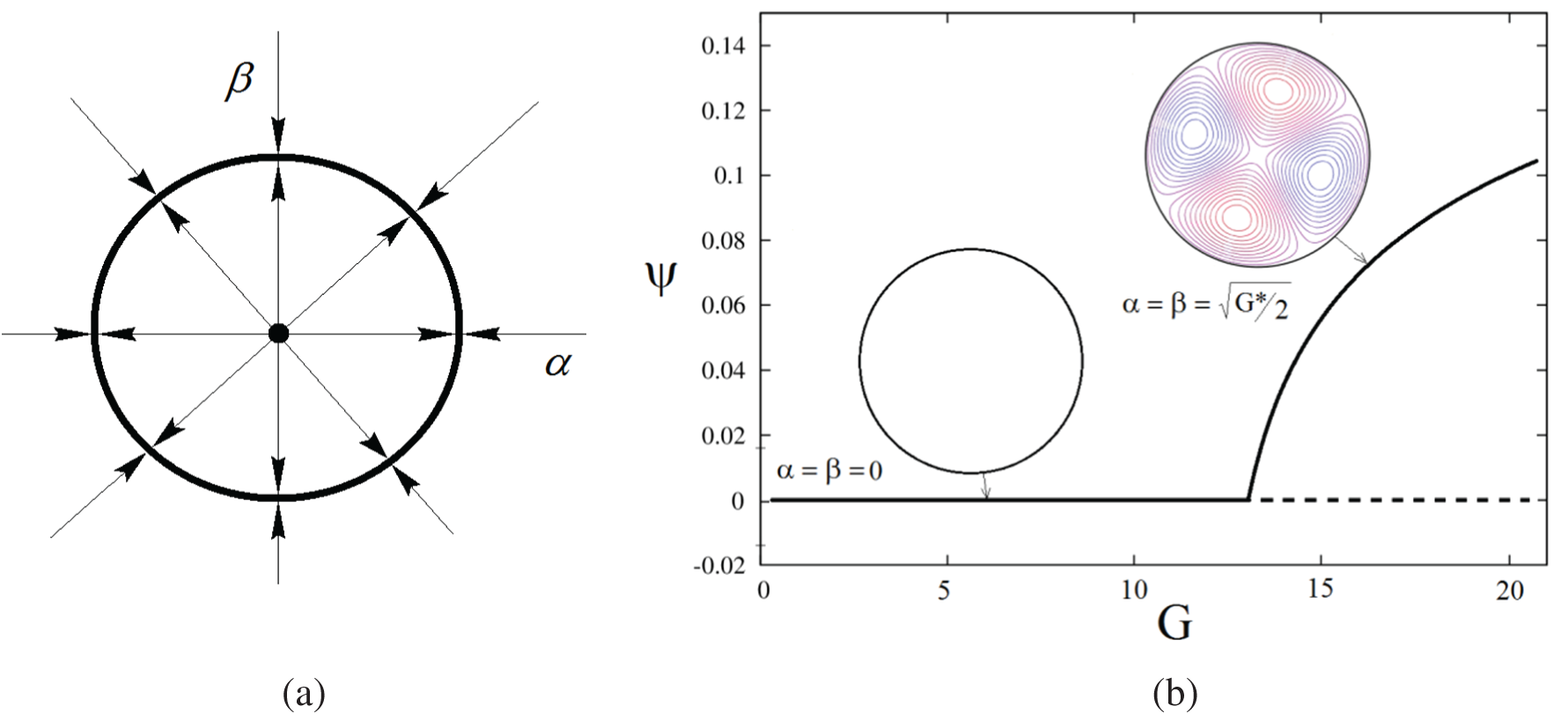
Figure 3: (а) Phase portrait of the dynamic system (27) for G* > 0; (b) Bifurcation diagram for steady-state solutions (27) on the line α = β
Finally, we note that the weakly nonlinear analysis presented in this section is only applicable near the first bifurcation point G0. We must keep in mind that as the swarm power increases, other modes also lose stability (see Table 1).
3.4 Direct Numerical Simulation
The nonlinear problem (11), (12) has been solved numerically by the finite difference method. We consider a circular domain of the radius r = 1. Spatial differential operators were approximated by central differences on a uniform mesh constructed in polar coordinates. We have used the series of meshes with different resolutions: 21 × 121, 41 × 241, 61 × 361, and 81 × 481. The numerical results presented below are obtained on the grid 61 × 361 (61 nodes in the radius and 361 nodes in the angle). We found that this grid network gives a result within 3% of the relative error of the value to which the stream function converges when the grid is improved.
The nonlinear equations are solved using an explicit scheme. For the time derivative, we used the Euler scheme with the order of O(Δt + Δhr + Δhφ), where Δt, Δhr, and Δhφ stand for the step in time, radius, and angle, respectively. Let us denote the discrete analog of the function f(t, r, φ) as fi,km, which gives the value of the function at the grid point i, k and at time tm = Σ Δtm. Let the indices i, k number the grid nodes in terms of radius and angle, respectively. Then finite-difference equations obtained from Eq. (11) have the following form:
The sequence of events during the operation of the computational scheme is as follows. Let at moment tm we know both fields: ψi,km and θi,km. At the very beginning, we perform an iterative solution of Poisson’s Eq. (30), the result of which is the determination of the stream function ψi,km+1. Then, using explicit recurrent Eq. (31), we can obtain values for temperature at a new time step: θi,km+1. Then the procedure is repeated for the next time step.
The Poisson equation for the stream function (30) was solved by the iterative Liebman successive over-relaxation method at each time step: the accuracy of the solution was fixed to 10−4. A noisy stream function field with amplitude less than 10−3 was used in the initial condition.
When using the scheme (30), (31), one has to control the time step. To ensure the stability of the numerical scheme, we used Courant’s formula to calculate new time step at each iteration:
Generally, the problem (11), (12) is convenient for numerical analysis. Liebman’s procedure converged to a solution in several (5–10) iterations when reaching a steady state and in 1–2 iterations if the parameter continuation technique was used.
Numerical simulation confirmed the conclusion of the linear theory and weakly nonlinear analysis: up to the critical value G0 = 13.21, all disturbances in the system decay. Just above the threshold, the steady-state solution representing the four-vortex circulation softly branches off from the trivial solution. As the control parameter increases, the circulation pattern becomes more complex. For example, at G = 14.3, one can observe a stationary circulation with already six symmetrical vortices (Fig. 4). Here, the distortions of the thermal field of the base state are already significant. These results agree with linear stability analysis, which predicts the branching of the 6-vortex structure when G > 13.57 (see Table 1). It is worth paying attention to the fact that the centers of the vortices are shifted to the edge of the swarm. It is explained by the fact that the magnitude of the temperature gradient increases as one approaches the edge of the domain. In fact, this is what generates the instability. In the center of a swarm, the temperature gradient becomes zero, which prevents instability from arising there.

Figure 4: Stream function of a finite-amplitude circulation of bots in a swarm at G = 14.3 obtained numerically. Red and blue vortices rotate clockwise and counterclockwise, respectively
As the parameter G increases further, more and more modes are included in the formation of the pattern. Finally, at G > 18.4, unsteady circulation develops in the system. The first oscillatory mode is a periodic restructuring of the circulation, in which 4-, 6-, and 8-vortex patterns sequentially appear and disappear. Fig. 5 shows the phase portrait of the system on the plane based on the maximum values of the stream function and temperature. As can be seen from the figure, at G > 21, the system exhibits chaotic behavior. The strange attractor appears after several Hopf bifurcations and a period-doubling cascade. One can see that the system ultimately moves to asymmetric circulation.

Figure 5: Phase portrait of a dynamic system (11), (12) on the plane of maximum values of the stream function and thermal field at G = 21. The inset shows the power spectrum of the signal. The corresponding temperature fields at different points of the attractor are shown on the right
When evaluating the results of a numerical simulation, one should recognize that the further from the first bifurcation point we are, the less realistic results we obtain. For large values of G, the shape of the swarm may become non-stationary, and bots are not bound only by the liquid state. Therefore, they can easily demonstrate the behavior of a gaseous medium, resulting in the decrease of the internal friction inside the swarm. In this case, the Darcy model (2) becomes unsuitable.
4 Final Discussion and Conclusions
Natural convection is a heat transfer mechanism in which the fluid motion is caused by buoyancy. The difference in fluid density occurs due to temperature or concentration gradients. Although gravity is necessary for the development of convection, the source of instability is the medium itself. Due to the inhomogeneity of the density field, the Archimedes force arises, which, under certain conditions, leads to fluid circulation. The excitation of natural convection from the point of view of physics has a simple meaning: an open system receives energy from the outside in the form of a heat gradient or concentration. With an increase in energy flow, the physical system is forced to switch to a convective heat transfer mechanism. Physicists say that the system is undergoing a second-order phase transition. The medium fluidity is a crucial factor in the process, as it allows the system to form a structure that serves the energy flow more efficiently.
Bioconvection is traditionally perceived primarily as the instability of a heterogeneous medium consisting of a huge number of microscopic living elements. Although classical bioconvection is an isothermal process, a natural convection specialist can easily understand the phenomenon. The ability of bacteria to self-propelate is a mechanism that generates density differences in the medium. It again leads to the appearance of buoyancy force under gravity. If the bacterial concentration gradient rises above a threshold value, convection occurs, which is not fundamentally different from natural convection in a purely physical system. From a biological perspective, the phase transition to complex circulation allows bacteria to gain access to a resource necessary for the collective survival of the entire colony.
It has become clear recently that the bioconvection phenomenon can also occur in higher animals. Emperor penguins provide us with an excellent example of this kind. When the external temperature sharply drops, these birds gather in a dense flock, demonstrating sporadic circulations. It allows penguins to create a collective thermal field in which, with periodic circulation, individuals warm themselves. As a result, the entire population survives. The value of this example lies in the fact that a flock of penguins consists of tens or hundreds of individuals, and each individual is a multicellular creature endowed with complex behavior (compared to a bacterium). However, the physical principles of natural convection work perfectly in this case, forcing these creatures to act simply but reliably for collective survival.
Inspired by this example, in this work, we decided to go even further and theoretically consider a swarm of artificial macroscopic elements. These bots can be programmed to perform simple actions that reproduce the conditions for fluidization of the swarm and the initiation of thermal convection. It is important to emphasize that the effect is possible even for a group limited in the number of bots. The results obtained in this work should be further supported by the development of a microscopic model. We also hope that the effect will be reproduced experimentally. This problem is fundamental since it demonstrates the power and universality of physical principles.
In conclusion, we proposed a mathematical model of self-organization in a dense medium of heat-generating bots that move along the gradient of the general thermal field. Linear stability analysis of the base state and weakly nonlinear analysis of the branching of steady-state solutions near the point of the first bifurcation are carried out analytically. We demonstrate that, as the power of the swarm increases, the phase transition of the 2nd order occurs, which leads to the excitation of stationary flows of bots.
Acknowledgement: The authors would like to thank the reviewers and editors for their useful suggestions for the improvement in the quality of our manuscript.
Funding Statement: This work was supported by the Ministry of Science and Higher Education of the Russian Federation (Project No. FSNM-2023-0003).
Author Contributions: Conceptualization, D.B.; software, K.K.; validation, K.K.; analytical study, D.B. and K.K.; supervision, D.B.; writing—original draft preparation, K.K.; writing—review and editing, D.B.; funding acquisition, D.B. All authors reviewed the results and approved the final version of the manuscript.
Availability of Data and Materials: The data that support the findings of this study are available from the corresponding author upon reasonable request.
Conflicts of Interest: The authors declare that they have no conflicts of interest to report regarding the present study.
References
1. Vicsek T, Zafeiris A. Collective motion. Phys Rep. 2012;517(3–4):71–140. doi:10.1016/j.physrep.2012.03.004. [Google Scholar] [CrossRef]
2. Whitesides GM, Grzybowski B. Self-assembly at all scales. Sci. 2002;295(5564):2418–21. doi:10.1126/science.1070821. [Google Scholar] [PubMed] [CrossRef]
3. Ozin GA, Arsenault AC. Nanochemistry: a chemical approach to nanomaterials. Cambridge, UK: Royal Society of Chemistry; 2005. [Google Scholar]
4. Wadhams GH, Armitage JP. Making sense of it all: bacterial chemotaxis. Nat Rev Mol Cell Biol. 2004;5:1024–37. doi:10.1038/nrm1524. [Google Scholar] [PubMed] [CrossRef]
5. Gregor T, Fujimoto K, Masaki N, Sawai S. The onset of collective behavior in social amoebae. Sci. 2010;328(5981):1021–25. doi:10.1126/science.1183415. [Google Scholar] [PubMed] [CrossRef]
6. Tabassum D, Polyak K. Tumorigenesis: it takes a village. Nat Rev Cancer. 2015;15(8):473–83. doi:10.1038/nrc3971. [Google Scholar] [PubMed] [CrossRef]
7. Bratsun DA, Krasnyakov IV, Pismen LM. Biomechanical modeling of invasive breast carcinoma under a dynamic change in cell phenotype: collective migration of large groups of cells. Biomech Model Mechanobiol. 2020;19:723–43. doi:10.1007/s10237-019-01244-z. [Google Scholar] [PubMed] [CrossRef]
8. Krasnyakov I, Bratsun D. Cell-based modeling of tissue developing in the scaffold pores of varying cross-sections. Biomimetics. 2023;8(8):562. doi:10.3390/biomimetics8080562. [Google Scholar] [PubMed] [CrossRef]
9. Hillesdon AJ, Pedley TJ. Bioconvection in suspensions of oxytactic bacteria: linear theory. J Fluid Mech. 1996;324:223–59. doi:10.1017/S0022112096007902. [Google Scholar] [CrossRef]
10. Giometto A, Altermatt F, Maritan A, Stocker R, Rinaldo A. Generalized receptor law governs phototaxis in the phytoplankton Euglena gracilis. Proc Natl Acad Sci USA. 2015;112(22):7045–50. doi:10.1073/pnas.1422922112. [Google Scholar] [PubMed] [CrossRef]
11. Bratsun DA, Zakharov AP. Modelling spatio-temporal dynamics of circadian rhythms in Neurospora crassa. Comput Res Model. 2011;3(2):191–213. doi:10.20537/2076-7633-2011-3-2-191-213. [Google Scholar] [CrossRef]
12. Al-Khaled K, Khan SU, Khan I. Chemically reactive bioconvection flow of tangent hyperbolic nanoliquid with gyrotactic microorganisms and nonlinear thermal radiation. Heliyon. 2020;6(1):e03117. doi:10.1016/j.heliyon.2019.e03117. [Google Scholar] [PubMed] [CrossRef]
13. Alharbi FM, Naeem M, Zubair M, Jawad M, Jan WU, Jan R. Bioconvection due to gyrotactic microorganisms in couple stress hybrid nanofluid laminar mixed convection incompressible flow with magnetic nanoparticles and chemical reaction as carrier for targeted drug delivery through porous stretching sheet. Molecules. 2021;26(13):3954. doi:10.3390/molecules. [Google Scholar] [CrossRef]
14. Javadi A, Arrieta J, Tuval I, Polin M. Photo-bioconvection: towards light control of flows in active suspensions. Philos Trans R Soc A. 2020;378:20190523. doi:10.1098/rsta.2019.0523. [Google Scholar] [PubMed] [CrossRef]
15. Ramamonjy A, Brunet P, Dervaux J. Pattern formation in photo-controlled bioconvection. J Fluid Mech. 2023;971:A29. doi:10.1017/jfm.2023.402. [Google Scholar] [CrossRef]
16. Saranya S, Ragupathi P, Al-Mdallal Q. Analysis of bioconvective heat transfer over an unsteady curved stretching sheet using the shifted Legendre collocation method. Case Stud Therm Eng. 2022;39:102433. doi:10.1016/j.csite.2022.102433. [Google Scholar] [CrossRef]
17. Saranya S, Al-Mdallal QM, Animasaun IL. Shifted Legendre collocation analysis of time-dependent Casson fluids and Carreau fluids conveying tiny particles and gyrotactic microorganisms: dynamics on static and moving surfaces. Arab J Sci Eng. 2023;48(3):3133–55. doi:10.1007/s13369-022-07087-8. [Google Scholar] [CrossRef]
18. Khan MI, Upadhyay TC. Study of structural order-disorder thermal dependence dielectric properties for PbHPO4 and PbHAsO4 crystals. Eur Phys J D. 2021;75:156. doi:10.1140/epjd/s10053-021-00171-y. [Google Scholar] [CrossRef]
19. Sumpter DJ. Collective animal behavior. Princeton, USA: Princeton University Press; 2010. [Google Scholar]
20. Ancel A, Visser H, Handrich Y, Masman D, Le Maho Y. Energy saving in huddling penguins. Nat. 1997;385:304–5. doi:10.1038/385304a0. [Google Scholar] [CrossRef]
21. Gerum RC, Fabry B, Metzner C, Beaulieu M, Ancel A, Zitterbart DP. The origin of traveling waves in an emperor penguin huddle. New J Phys. 2013;15(12):125022. doi:10.1088/1367-2630/15/12/125022. [Google Scholar] [CrossRef]
22. Richter S, Gerum R, Winterl A, Houstin A, Seifert M, Peschel J, et al. Phase transitions in huddling emperor penguins. J Phys D Appl Phys. 2018;51(21):214002. doi:10.1088/1361-6463/aabb8e. [Google Scholar] [PubMed] [CrossRef]
23. Bratsun D, Kostarev K. A continuum model of bioconvection with a centripetal force. Phys. 2022;2:36–46 (In Russian). doi:10.17072/1994-3598-2022-2-36-46. [Google Scholar] [CrossRef]
24. Solem JC. Self-assembling micrites based on the Platonic solids. Robot Auton Syst. 2002;38(2):69–92. doi:10.1016/s0921-8890(01)00167-1. [Google Scholar] [CrossRef]
25. Zampetakia AV, Liebchen B, Ivlev AV, Löwen H. Collective self-optimization of communicating active particles. Proc Natl Acad Sci USA. 2021;118(49):e2111142118. doi:10.1073/pnas.2111142118. [Google Scholar] [PubMed] [CrossRef]
26. Rubenstein M, Cornejo A, Nagpal R. Programmable self-assembly in a thousand-robot swarm. Sci. 2014;345(6198):795–99. doi:10.1126/science.1254295. [Google Scholar] [PubMed] [CrossRef]
27. Leaman EJ, Geuther BQ, Behkam B. Hybrid centralized/decentralized control of a network of bacteria-based bio-hybrid microrobots. J Micro-Bio Robot. 2019;15(1):1–12. doi:10.1007/s12213-019-00116-0. [Google Scholar] [CrossRef]
28. Slavkov I, Carrillo-Zapata D, Carranza N, Diego X, Jansson F, Kaandorp J, et al. Morphogenesis in robot swarms. Sci Robot. 2018;3(25):eaau9178. doi:10.1126/scirobotics.aau9178. [Google Scholar] [PubMed] [CrossRef]
29. Crank J. The mathematics of diffusion. Oxford, UK: Clarendon Press; 1975. [Google Scholar]
30. Nield D, Bejan A. Convection in porous media. New York, USA: Springer Cham; 2017. doi:10.1007/978-3-319-49562-0. [Google Scholar] [CrossRef]
31. Gershuni GZ, Zhukhovitsky EM. Convective stability of incompressible fluids. Jerusalem, Israel: Keter Publishing House; 1976. [Google Scholar]
32. Bratsun DA, Lyubimov DV, Roux B. Co-symmetry breakdown in problems of thermal convection in porous medium. Physica D. 1995;82(4):398–417. doi:10.1016/0167-2789(95)00045-6. [Google Scholar] [CrossRef]
Cite This Article
 Copyright © 2024 The Author(s). Published by Tech Science Press.
This work is licensed under a Creative Commons Attribution 4.0 International License , which permits unrestricted use, distribution, and reproduction in any medium, provided the original work is properly cited.
 Downloads
 Citation Tools