
 Submit a Paper
 Propose a Special lssue
 Open Access
ARTICLE
Exploring Capillary Fringe Flow: Quasilinear Modeling with Kirchhoff Transforms and Gardner Model
1 LASTIMI Laboratory, Mohammadia School of Engineers, Mohammed V University in Rabat, Rabat, Morocco
2 LIRNE Laboratory, Faculty of Sciences, Ibn Tofail University, Kenitra, Morocco
* Corresponding Author: Rachid Karra. Email:
Fluid Dynamics & Materials Processing 2024, 20(7), 1611-1631. https://doi.org/10.32604/fdmp.2024.048447
Received 08 December 2023; Accepted 13 March 2024; Issue published 23 July 2024
 View Full Text
 Download PDF
Abstract
Recent studies have underscored the significance of the capillary fringe in hydrological and biochemical processes. Moreover, its role in shallow waters is expected to be considerable. Traditionally, the study of groundwater flow has centered on unsaturated-saturated zones, often overlooking the impact of the capillary fringe. In this study, we introduce a steady-state two-dimensional model that integrates the capillary fringe into a 2-D numerical solution. Our novel approach employs the potential form of the Richards equation, facilitating the determination of boundaries, pressures, and velocities across different ground surface zones. We utilized a two-dimensional Freefem++ finite element model to compute the stationary solution. The validation of the model was conducted using experimental data. We employed the OFAT (One_Factor-At-Time) method to identify the most sensitive soil parameters and understand how changes in these parameters may affect the behavior and water dynamics of the capillary fringe. The results emphasize the role of hydraulic conductivity as a key parameter influencing capillary fringe shape and dynamics. Velocity values within the capillary fringe suggest the prevalence of horizontal flow. By variation of the water table level and the incoming flow q, we have shown the correlation between water table elevation and the upper limit of the capillary fringe.Keywords
Nomenclature
| | The Gardner model parameter depends on the size and distribution of pores |
| | Relative conductivity exponent |
| | Volumetric water content scale parameter, which is called the volumetric water content at natural saturation |
| | Residual water content |
| | Air-entry pressure is defined as the suction pressure at which air begins to move water from the pores (appearance of first bubbles) |
| | Hydraulic conductivity |
| | Saturated hydraulic conductivity |
| | Matric flux potential |
| | Effective particle diameter |
| n | Porosity |
The capillary fringe represents a highly dynamic region situated at the interface between the unsaturated zone and the water table, where significant hydrological and geochemical gradients are anticipated [1]. Early studies omitted the inclusion of the capillary fringe in modeling groundwater flow; it was regarded as an inconsequential zone with no discernible impact on the hydrological cycle and, consequently, on physical and biological activities. Instead, researchers concentrated on a combination of the vadose and saturated zones. Groundwater recharge acts as the primary driving force behind the transportation of contaminants, such as nutrients and pesticides, to the water table. Owing to its distinctiveness, the capillary fringe remains a challenging area for study.
The capillary fringe is increasingly recognized for its substantial role in the generation of stream flow, influencing both the volume and swiftness of water mobilization [2]. During rainfall events, limited water intake can swiftly elevate the water table, significantly altering local hydraulic gradients. Notably, the capillary fringe serves as a vital source for pre-event streamflow and groundwater ridging. When this zone extends to the ground surface, even a small water volume triggers rapid stream groundwater ridge formation and subsurface discharge into the stream, a phenomenon described as the ‘Reverse Wieringermeer Effect’ [3]. This rapid elevation of the water table with minimal water input carries profound implications. Zheng et al. [4], in their investigation into the intersection of the capillary fringe with the surface, they propose that tidal pumping in sediments has a minimal effect. Although Gillham’s research contributes valuable insights into this mechanism, other field studies have not explicitly highlighted its significance in flood formation.
The influence of the capillary fringe on physical and biochemical activities is intricately tied to soil types and pore sizes, such as sand, gravel, or coarse textures. While some studies, like Ronen et al. [5], encompass relative water content as the upper limit or incorporate the saturation and near-saturation zones above the water table, a consensus on defining the capillary fringe remains elusive. Generally acknowledged as the zone above the water table where all pores exhibit full saturation under a negative pressure head [6], the capillary fringe’s characterization has varied. Despite its consideration in diverse natural settings such as coastal beaches and estuaries, comprehensive descriptions pertaining to two-dimensional variably saturated models are notably limited.
Another significant aspect of analyzing the capillary fringe pertains to its relationship with CO2 storage, one of the greenhouse gases contributing to climate change. Notably, the capillary fringe’s height can vary from a few centimeters in coarse materials to several meters in very fine materials, underscoring its importance in this context. However, experiments aiming to understand soil contamination involving stronger capillary forces approximations are less suitable [7]. Reference [8] mentions the pivotal role of the capillary fringe in governing groundwater dynamics across various scenarios. Beginning with the exploration of Managed Aquifer Recharge (MAR) systems, it underscores how fluctuations in the water table, particularly within the capillary fringe, can influence the release of persistent pollutants like per- and polyfluoroalkyl substances (PFAS). This highlights the critical need to understand capillary processes for effective groundwater management in urbanized areas facing water stress. There is a burgeoning interest in exploring the interactions and advancements regarding chemical and organic pollutants within the capillary fringe. Studies delve into various aspects, such as the biodegradation of aromatic components (e.g., Phenol, Benzenesulfonic acid C6H6O3S) and the investigation of oil contamination [9,10]. Similarly, researchers delves into the temporal and spatial dynamics of soluble arsenic (As) and cadmium (Cd) concentrations at the capillary fringe, particularly emphasizing the interface’s sensitivity to moisture-driven changes [11]. This elucidation of capillary processes provides valuable insights into strategies for mitigating contamination risks in paddy soils and enhancing food safety. The effectiveness of the biodegradation process relies on several factors, including the proportion of oxygenation, water content, and elements within the capillary fringe, necessitating a deeper understanding of its dynamics [12]. In our study, we utilized sandy soil characterized by a significant capillary rise, leading to a potential truncation between the capillary fringe and the root zone. Prolonged wet conditions over several days can stress roots and affect crop growth. Moreover, arid regions often experience soil salt accumulation, posing substantial challenges to agriculture under irrigation. Consequently, comprehending the capillary fringe’s role in shallow groundwater is crucial for managing surface salt accumulation issues. Integrating an efficient subsurface drainage system that considers the capillary fringe could provide more accurate diagnostics [13]. Such understanding is pivotal not only in addressing soil pollution but also in controlling soil salinity. Analysis of the Alazaiza et al. study [14] images reveals a time-dependent LNAPL distribution in the capillary fringe during the experiments, with higher diesel volumes showing faster migration due to increased pressure. The initial rapid migration gradually slowed down, attributed to the pressure allowing diesel percolation.
Investigating water movement within a porous environment, where saturation levels vary, poses a significant hurdle because of the intricate equations dictating exchanges between saturated and unsaturated zones. This intricacy stems from the need to address the interplay between vertical flow in the unsaturated zone and horizontal flow in the groundwater, compounded by the uncertainty surrounding the water table’s initial state. Furthermore, accurately delineating the upper boundary of the region between these domains, known as the capillary fringe, continues to be a persistent obstacle [6]. Sun et al.’s experiment [15] delves into the response of riparian groundwater flow systems to rainfall through a combination of laboratory experiments and numerical simulations. In the laboratory experiments, a 1D sand column was utilized, revealing a capillary fringe of 25 cm and a supporting capillary water height of approximately 65 cm. Furthermore, a 2D sandbox was employed to examine changes in hydraulic heads and groundwater flow patterns in a hypothetical riparian zone under varying initial water tables and rainfall intensities.
Neglecting the capillary fringe often leads to the consideration of primarily vertical flow above the water table. Comprehensive studies focusing on the capillary fringe are relatively scarce, primarily due to its inherent complexity and challenging accessibility, particularly in field conditions. Furthermore, the absence of detailed measurements significantly contributes to the misunderstanding surrounding this critical zone. To address this, the potential approach integrates the widely utilized Gardner model, as extensively documented in literature [16,17]. Its exponential formulation allows quasi-linearization of the Richards equation, making it applicable in both stationary and transient infiltration treatments. The model’s key parameter, αG, quantifies the significance of gravitational forces concerning capillary forces. At the field scale, this parameter is assumed to follow a log-normal distribution. Remarkably, beyond being a fitting parameter, its inverse,
In this study, we propose a numerical model that integrates the capillary fringe, aiming to simulate two-dimensional steady-state water flow in variably saturated porous media. Our assumption hinges upon the flow being both homogeneous and incompressible. While previous studies heavily relied on experiments and observations to delineate the limits of the capillary fringe (6), our model enabled a clear identification of its contours. Specifically, it allowed for the accurate determination of the upper limit demarcating the capillary fringe from the unsaturated zone, a task previously challenging to ascertain. Our pursuit of developing a physical model describing the capillary fringe dynamics is intended to deepen our comprehension of hydrological behavior and the consequential impact of the capillary fringe.
To achieve this goal, we employed the steady-state potential form of the Richards equation, treating both the unsaturated and saturated zones as a unified continuum. The numerical modeling in this study relies on the finite element code Freefem++, employing triangular elements [19]. Notably, the finite element program was meticulously adapted to encompass the equations by integrating boundary conditions and the sink term. The soil representation involves a uniform two-dimensional medium, with water characteristics defined by the Gardner model. To ensure the robustness and validity of our numerical model, rigorous validation against experimental data was undertaken.
2 Description of the Study Domain
The laboratory tests involved a soil slab with dimensions of 300 cm in length and 200 cm in depth. The source of flow was provided by a rainfall simulator confined within a steel rectangle, which targeted a specific infiltration band measuring 50 cm in width [20]. Utilizing naturally occurring fine sand sourced from the Mnasra region near Kenitra, Morocco, we employed it as a porous media for our experimentation. Extracted from a depth of 0 to 20 cm, the soil boasted 1.41% organic matter and comprised 82.75% sand content. Preliminary investigations, preceding our research, were dedicated to scrutinizing the fundamental attributes of this sand [21,22]. The foundational physical properties of the sand were characterized by αG = 0.018 and Ks = 0.01 cm/s. Prior to commencing the experiments, the sandbags underwent a meticulous process: they were carefully transported and systematically spread across expansive shelves to ensure uniform aeration. Throughout the drying period, meticulous attention was given to the removal of impurities such as small roots and debris, and the sand was consistently stirred. Following this preparatory phase, the sand was transferred to a basin. It was underwent saturation with water, effectively eliminating any trapped air within its porous structure. Subsequently, the water was drained into the tank, establishing a water table at precisely 65 cm in the reservoir.
To enforce a consistent hydraulic head at the outlet, a reservoir was connected to the slab. The soil is assumed to possess homogeneity, rigidity, and isotropy. We adopted a coordinate system xOz, with the Ox axis representing the ground surface and the positively oriented Oz axis directed downward, with point O situated at the center of the infiltration band. The soil surface is presumed to be flat, and we consider symmetry about the Oz axis, treating the problem as a planar one. In our setup, we established a horizontal water table positioned e units above an impermeable base at a depth of e0. To induce a consistent infiltration flow q0 across the ground surface, this condition was assumed. Additionally, we placed the reservoir between two parallel trenches of equal length to the slab, ensuring they maintained a uniform piezometric level at a fixed depth of e0. The utilization of a Marriotte bottle system effectively regulated and upheld a constant water table level at the outlet. For a visual representation, please refer to Fig. 1, depicting the system’s geometry:
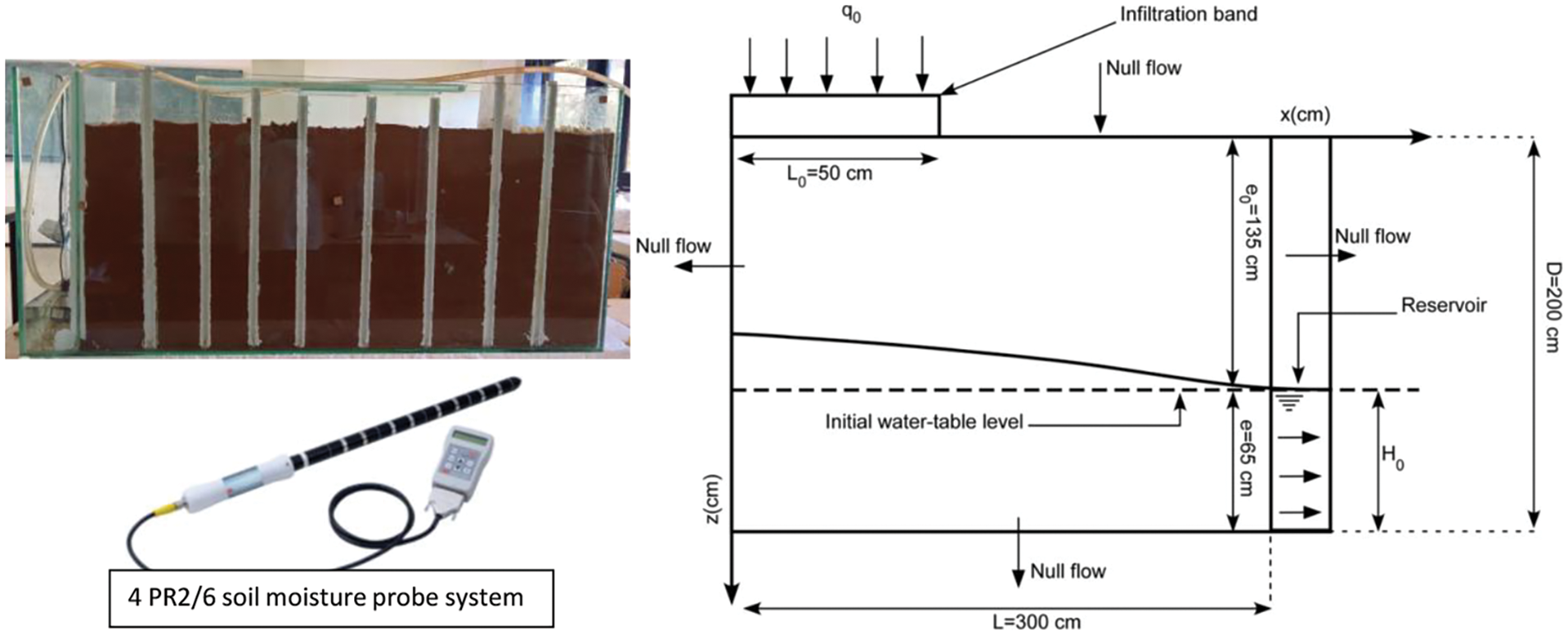
Figure 1: Flow domain schema
- A portion of the upper horizontal surface (ground level) undergoes the application of a constant flux q0 = 15 cm/h, mimicking an infiltration band resembling an irrigation canal or artificial catchment basin. The selected value of q0 was intentionally set below the saturated hydraulic conductivity of this particular soil.
- We utilize a nozzle rainfall simulator confined within a steel rectangle measuring 5 cm in height. Additionally, we establish a water table level at the outlet equivalent to H0. To mitigate mechanical disturbance to the soil structure during the hydrology experiment, we dispersed small stones across the surface of the infiltration strip, ensuring that the flow of water proceeded without disruption.
The process applied to fine sand ensures consistency and uniform distribution of grain sizes. We used 4 PR2/6 soil moisture probe system vertically in positions x = (100, 150, 210, 260 cm). The PR2/6 sensors remained securely positioned as sand was incrementally added. Care was taken to maintain their vertical alignment, ensuring proximity to the designated measurement points for accurate data collection.
Addressing the coupling problem between the unsaturated and saturated zones poses certain complexities, particularly in defining the boundary between these distinct areas. The water table’s free surface is identified by a null pressure head (h = 0), while the hydraulic head corresponds to the elevation head z (as illustrated in Fig. 1). Alternatively, the free surface can be delineated as the level where the flow becomes negligible, specifically in scenarios devoid of vertical recharge of groundwater through infiltration.
The unsaturated and saturated zones are considered as a cohesive continuum, divided by a capillary-dominant layer. Above the water table, there exists a zone with low capillary tension, leading to soil pores being nearly saturated with water while retaining a minimal amount of air. This transitional region is recognized as the capillary fringe, situated between the saturated and vadose zones [6]. The capillary fringe, extending vertically, significantly influences the soil’s water profile and surface runoff dynamics. Its pivotal role lies in determining the volume of water that infiltrates into the groundwater vs. that which runs off at the surface. Within this area, capillary flow mechanisms operate as well. In cases where the capillary rise is significant, it may ascend to the extent of reaching the root zone. The thickness of the capillary fringe corresponds to the air-entry pressure value, indicating the suction needed for air to penetrate the pores.
According to Youngs [13] and Childs, the capillary fringe is defined as the region above the water table, characterized by uniform moisture content and hydraulic conductivity closely resembling that of the saturated zone [15].
The delineation between the unsaturated zone and the capillary fringe exhibits non-linearity and lacks a perfectly straight boundary. On a closer inspection of the upper limit curve at a finer scale, distinct irregularities become apparent. Fig. 2 depicts this curve’s variance around the mean value he, validating this widely adopted approximation. In the capillary fringe, the spaces between pores are completely saturated, reflecting the moisture level at saturation. The key difference between this zone and the saturated region lies in the negative pressure within the pores, which remains lower than atmospheric pressure.
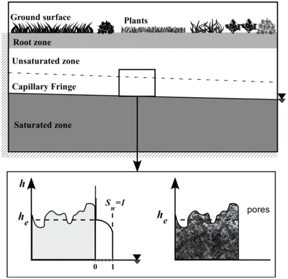
Figure 2: Illustration of the capillary fringe in hypothetical domain; he the air entry pressure; Sw the effective saturation
In the subsequent section, our focus will be on modeling flux within the unsaturated zone using the potential form of the Richards equation. Leveraging Gardner’s exponential model aids in mitigating the equation’s nonlinearity. Zone boundaries are defined in terms of potentials, and upon resolving the potential equations, we apply Kirchhoff’s inverse transform to determine the distribution of pressure and hydraulic head.
Several empirical models are employed to describe the hydrodynamic properties of soil, establishing relationships among water content, pressure head, and hydraulic conductivity [23]. These models utilize specific parameters that characterize various soil types. One of the earliest widely adopted models is Gardner’s, which formulates soil properties exponentially and was modified by [24]. The residual moisture content θres is disregarded due to its minimal quantity of moisture content θ. Here, H[L] denotes the pressure head. The effective saturation Se(h) is expressed as follows:
and the hydraulic conductivity by:
αG measures the relative significance of gravity against capillary forces within porous media. The determination of he involves calculating it through theoretical or experimental relations. Rucker et al. [18] suggest a different method for determining the dimensionless air-entry pressure head using the van Genuchten parameter, taking into account different relative hydraulic conductivity values.
3.3 Flow Equation in the Unsaturated Zone
Neglecting the compressibility of water, the steady-state flow in the unsaturated soil is based on the 2D Richards equation:
where S is a sink/source term
To have a potential form the Richards equation, we use the Kirchhoff integral transformation [17,25], defined below, on (3):
With
We use the Leibniz’s rule for differentiation with one variable:
The combination of the Gardner model and the Kirchhoff potential formula is:
Combining Eqs. (3), (6) and (7), we obtain the potential form of the Richards equation characterizing the steady state flow in the unsaturated zone:
3.4 Flow in the Saturated Zone and the Capillary Fringe
We will derive an equation governing the flow based on the discharge potential in both the capillary fringe and the saturated zone. The application of the same equation to these zones is justified by the saturated nature of the pores within the capillary fringe. As highlighted by Luthin et al. [26], the use of the Laplace equation is suitable for analyzing flow patterns within the capillary fringe. Subsequently, in line with the approach proposed by Wong et al. [27], we formulate the problem in terms of discharge potential:
Darcy’s law expresses relate the volumetric flux
thus, in combination with the mass conservation law:
implies:
The potential must satisfy Laplace’s equation in the saturated zone.
As observed, the sole distinction between the Richards equation in the unsaturated zone and that in the capillary fringe and saturated zone lies in a specific term
In general, throughout the domain, the potential must be finite, continuous everywhere and vanish at infinity. The boundary conditions on the surfaces are as follows:
On both sides of the area, we have a null horizontal flow,
Along the bottom, the vertical flow is null, so:
For x=0 and outside the infiltration strip, the flow is null
The vertical flow imposed on the infiltration band:
Along the outlet, a constant hydraulic head was specified,
After solving the problem in terms of potential, our next step involves establishing the relationship between pressure head and potential. Upon substituting Kirchhoff potential into the expression for the hydraulic conductivity function (Eq. (2)), the resulting equation is derived, as described by Bakker et al. [16] and Ameli et al. [30]:
with:
The pressure head h becomes:
At saturation and based on Eq. (9), the pressure is:
The Darcy flow vector expressed in terms of the potential:
3.7 The Limit between the Unsaturated Zone and the Capillary Fringe
Our determination of the boundary between the unsaturated and saturated zones is reliant on their respective definitions. In describing the unsaturated zone, we utilize both the pressure head and the water content:
Based on Gardner model:
Because βG > 0 and replacing the pressure
Hence:
Transferring Eq. (20) into Eq. (26) and since
The boundary between the capillary fringe and the saturated zone is clearly defined by the water table.
The principal aim of this study is to model the capillary fringe employing the potential method. To achieve this objective, we utilized a dedicated code designed to compute both flux and hydraulic heads based on the φ-based equation. This entailed using mathematical models to solve two-dimensional partial differential equations (PDEs) and their associated boundary conditions through numerical simulations. We utilized the Galerkin finite element method along with Freefem++ software to tackle the equations of the system effectively.
The outline of the field of study is divided into six parts. The flow is zero everywhere except in the infiltration inlet at the top and the outlet of the slab (reservoir). We initially solve the equation in Kirchhoff potential, then we convert the potential into hydraulic pressure depending on whether the flow is governed by Eq. (8) of the unsaturated zone or Eq. (12) of the capillary fringe and saturated zones. A constant load at the output equals:
The problem: Find u a real function defined in
We iteratively refined the mesh until observing no further variations in the solution. However, it is important to note that an excessively fine mesh may lead to convergence issues. Our initial spatial discretization of the flow domain utilized an unstructured triangular mesh, comprising 770 elements and 426 vertices (see Fig. 3). The statistics of the adaptive mesh are Nb of Triangles = 2188, Nb of Vertices 1157 and area = 60000.
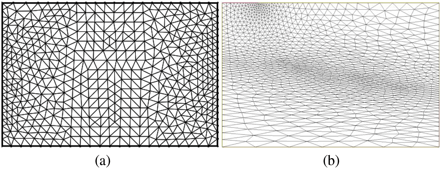
Figure 3: (a) Initial mesh. (b) Refined mesh using adaptive meshing
For visualization the results are exported to .eps format. For this study’s purpose, we modified and tailored the code to address water flow challenges in unsaturated-saturated porous media. We utilized a polynomial space Wh with a 0-degree for the flux and Vh 1-degree for the pressure, water content, and hydraulic head.
To validate the model, we compared the calculated groundwater water table level with experimental measurements, utilizing αG = 0.018 and Ks = 0.01 cm/s, obtained from the steady-state condition (19). Fig. 4 displays the profile of the simulated water table generated by the numerical model alongside measurements obtained after reaching a steady state within 8 h. Remarkably, the results exhibit a good level of consistency, showcasing a low error rate. The experimental measurements taken for the upper limit of the capillary fringe (nearly at saturation) align impeccably with the predictions of the numerical model.
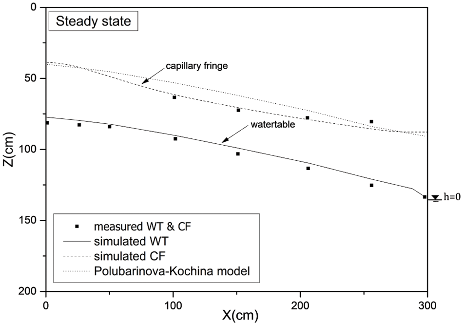
Figure 4: The measured and simulated level of water table and the two capillary fringe upper limit models
Polubarinova-Kochina [31] proposed the following relationship as a means to determine the height of capillary rising:
Fig. 4 depicts a significant concurrence between the two models, although limitations arise with the constant value utilized in the Polubarinova-Kochina model. This constant fails to accurately represent variations in the capillary fringe height, particularly within the middle zone. In proximity to the outlet, an irregularity in the pressure head curve is noticeable, stemming from the absence of a seepage surface in our model. This absence prompts a swift approach of the pressure head to zero at the outlet, whereas measurements indicate a mere few centimeters of difference. Notwithstanding these observations, our model demonstrates a commendable alignment with experimental data, affirming its efficacy in capturing experimental behavior.
We evaluated our model’s performance using statistical indicators, as outlined by [32]. The assessment included comparing the root mean square error RMSE to the mean measured value and employing the normalized root mean square error NRMSE as an indicator of the goodness of fit. These metrics are defined as follows:
The RMSE value of 3.39 cm signifies a minimal difference between observed and calculated values, highlighting the model’s accuracy. Furthermore, the R2 indicator reaching 0.99, as depicted in Fig. 5, underscores the model’s impressive performance. Additionally, the NRMSE, expressed without dimension at 0.03, emphasizes the model’s high precision. Estimating the model’s uncertainty further supports its robust performance, confirming its accurate prediction of the water table level. It is important to note that the precision of the hydraulic parameters significantly impacts the accuracy of the model’s results.
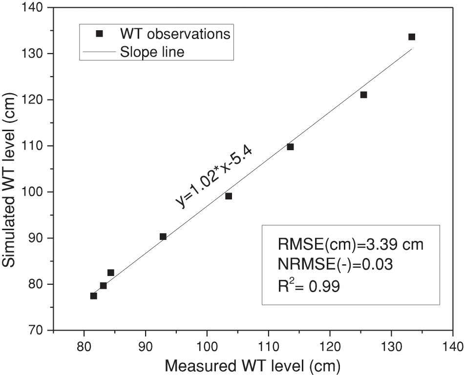
Figure 5: Statistical indicators of the hydrodynamic model performance
The main parameters to test are the saturated hydraulic conductivity Ks and αG. The evaluation of the variation effect of each parameter is important to determine which measurement must be made with great precaution.
4.2 Thickness of the Capillary Fringe
The thickness of the capillary fringe is associated with the particle size distribution of soils and is influenced by flow dynamics. Fig. 6 illustrates the variations in capillary fringe thickness, displaying the mean values across the three zones.
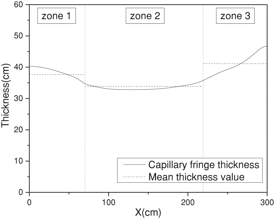
Figure 6: Spatial variation of the capillary fringe thickness
The thickness of the capillary fringe varies across the schema, with its greatest thickness observed in the infiltration band and at the outlet (with a fixed charge H0), surpassing the middle section (zone 2). Changes in the mean thickness depend on the conditions affecting the fringe. This disparity among the three zones highlights the model’s effectiveness in depicting the genuine dynamics of the fringe, surpassing the limitations of a simplistic static model [32]. Significantly, the thickness variation within zone 2 remains constrained. In contrast, there is considerable disparity observed in the other two zones relative to their midpoint, highlighting the heightened importance of the capillary fringe in shallow waters (near the surface) and within the Intertidal and supratidal zones.
The employed method involves systematically adjusting each entry parameter of the model by both −10% and +10% around its initial value. This percentage range is deemed acceptable, considering the inherent inaccuracies associated with the model’s input parameters.
Subsequently, the percentage of variation and sensitivity index [33] are computed using data derived from the water table and the capillary fringe. These values are determined by the following formulas:
SI the sensitivity index.
Ei the inputs, Eavg the average.
Si the outputs, Savg the average.
This index serves as a quantitative measure to express the sensitivity of the model outputs concerning changes in the input variables. Specifically, we opted to analyze the soil characteristics for sensitivity assessment. The outcomes of this sensitivity analysis for both the water table and the capillary fringe are detailed in Table 1.
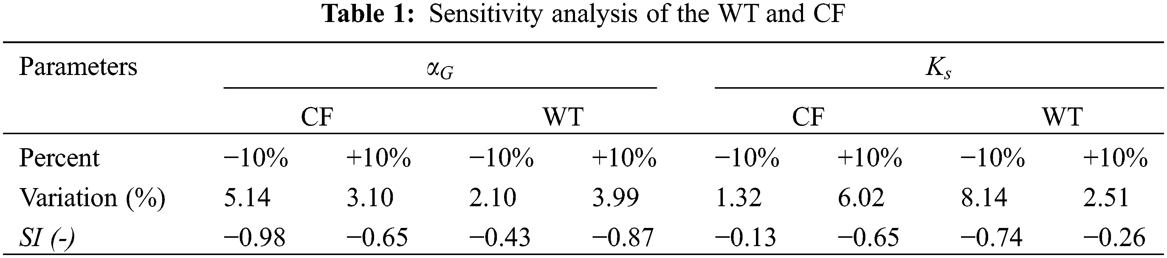
Fig. 7 shows the sensitivity analysis of the
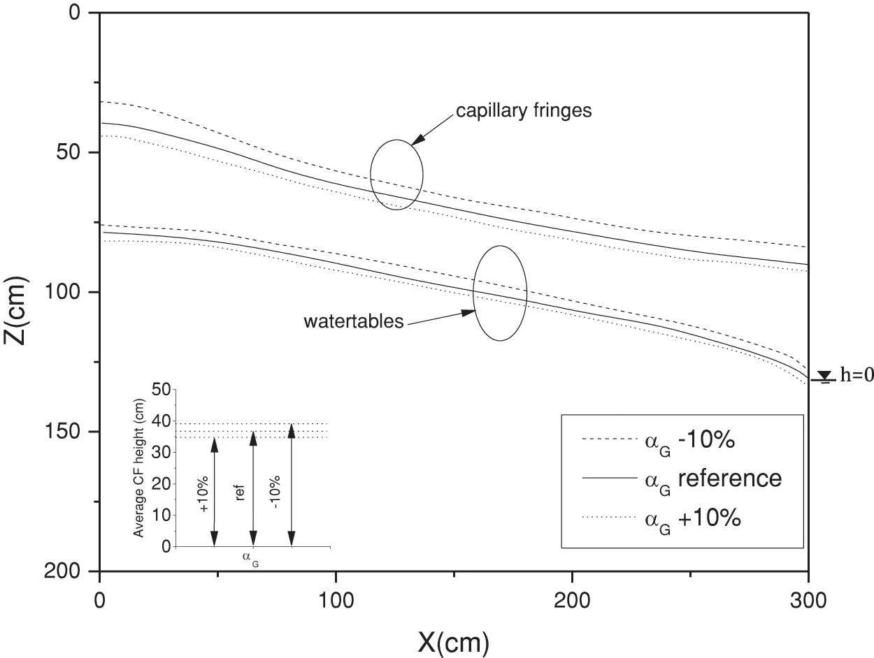
Figure 7: Sensitivity analysis of the water table and upper limit CF position relative to αG at steady state
Modifying inputs by ±10% induces output variations of approximately 5% for the capillary fringe and between 2% to 4% for the water table. Across the domain’s x-axis, the variation is uniformly distributed. Notably, a ± 10% alteration in αG exhibits a corresponding impact on the rate of change in capillary fringe height.
The negative Sensitivity Index (SI) for the capillary fringe signifies an inverse relationship between αG and the capillary fringe level. Specifically, an SIcf−10% near –1 implies that a variation in αG results in a proportional variation in the output. Comparatively, the SIcf+10% exhibits a lower variation rate than the SIcf−10%.
Similarly, the negative SI for the water table indicates an inverse relationship between αG and the water table level. With an SIwt−10% near −0.43, the variation rate between αG and the water table level is roughly half of the output’s rate variation.
In our analysis, we conducted a sensitivity test on the saturated hydraulic conductivity Ks, as illustrated in Fig. 8. A −10% adjustment in Ks results in an output variation of approximately 1.3% for the capillary fringe, while a +10% modification causes a 6% variation. Similarly, altering Ks by +10% or −10% leads to a water table level variation of 2.51% and 8.14%, respectively. Remarkably, the most significant variance is observed within “zone 1”, gradually tapering off towards the outlet. Conversely, in “zone 2”, the variance is evenly dispersed across the x-axis. This finding indicates a diminishing lateral impact of hydraulic conductivity with increasing distance from the infiltration band or water source.
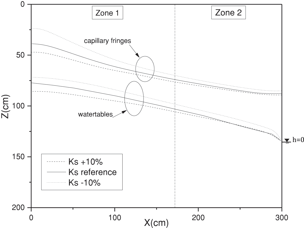
Figure 8: Sensitivity analysis of the water table and the capillary fringe upper limit position relative to Ks at steady state
Furthermore, a decrease of Ks by −10% induces a more pronounced change in the capillary fringe height compared to an increase of +10%. In instances of low soil permeability, the capillary fringe might ascend closer to the surface, particularly during the rainy season. However, it is crucial to prevent scenarios where the capillary fringe reaches the root zone, as plant roots require both water and air for optimal growth.
The negative Sensitivity Index (SI) for both the capillary fringe and the water table indicates a reverse correlation between the saturated hydraulic conductivity (Ks) and the elevation level. Interestingly, it is noted that for an equivalent rate of change, the rise in the water table level surpasses its decline. This discrepancy is due to the imposed hydraulic head at the outlet, which restricts a proportional decrease. Notably, a −10% variation in Ks yields a change in the capillary fringe elevation of a certain magnitude, half that observed with a +10% variation. The SIwt−10% value stands at 0.7, indicating that the variation rate of Ks leads to about two-thirds of the variation rate in the output. These findings from the sensitivity analysis underscore the pivotal role of hydraulic conductivity as a key parameter influencing capillary fringe dynamics.
The pore water content is defined either by the volumetric water content or by the effective saturation. It is defined to scale the range between 0 and 1 and determined by the classical hydraulic parameters θ(h), θr, θs. Typically, Se-h data is less difficult to measure than K-h.
The function of effective saturation Se concerning depth is visualized in Fig. 9. Notably, the effective saturation Se experiences a rapid decline below unity. Typically, the upper boundary of the capillary fringe occurs at Se = 95%, with a significant portion of it at full saturation. The inflection points visible in the characteristic curve near saturation levels correspond to the air entry barrier for the initial formation of bubbles. To trace the water content at various positions (x(cm) = 0, 130, 300), it was compared with the upper limit of the capillary fringe. This comparison revealed a correlation between the effective saturation ranging from 95% to 100% and the anticipated height of the capillary fringe.
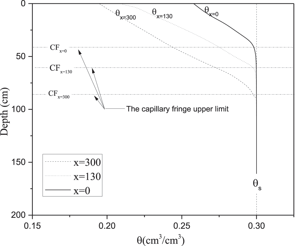
Figure 9: Effective saturation vs. depth for different x values
Effective saturation serves as a useful indicator to establish the boundary between the unsaturated zone and the capillary fringe. However, it does not provide indications about the limit between the saturated zone and the capillary fringe (refer to Fig. 10). In the capillary fringe, effective saturation maintains a proportionality to θ (water content). Notably, a significant portion of the capillary fringe remains at full saturation (Se = 1), with exceptions in certain areas near the upper limit where the effective saturation slightly decreases below unity.
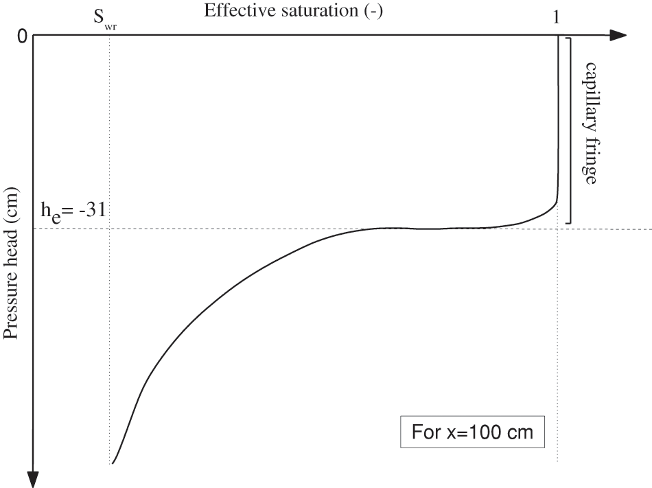
Figure 10: Effective saturation vs. pressure head
Displayed in Fig. 11 are the spatial distributions of hydraulic head and pressure head. The model effectively simulates water flow across the two unsaturated-saturated zones, encompassing the integration of the capillary fringe.
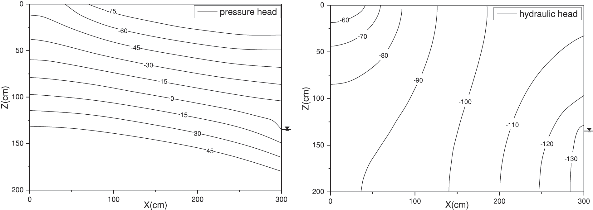
Figure 11: Simulated hydraulic head and pressure head at steady state
The thickness of the capillary fringe is markedly greater at the vertical level aligned with the infiltration band compared to its midpoint. This variation arises from heightened capillary forces exerted in this area, driven by substantial water movement. Upon reaching a steady state, the water table stabilizes at its maximum position. At this stage, the domain achieves hydrostatic balance, resulting in an equilibrium where the influx through the infiltration band matches the outflow through the aquifer’s outlet. The findings from Fig. 12 affirm that the flow velocity aligns with the direction of potential decrease.
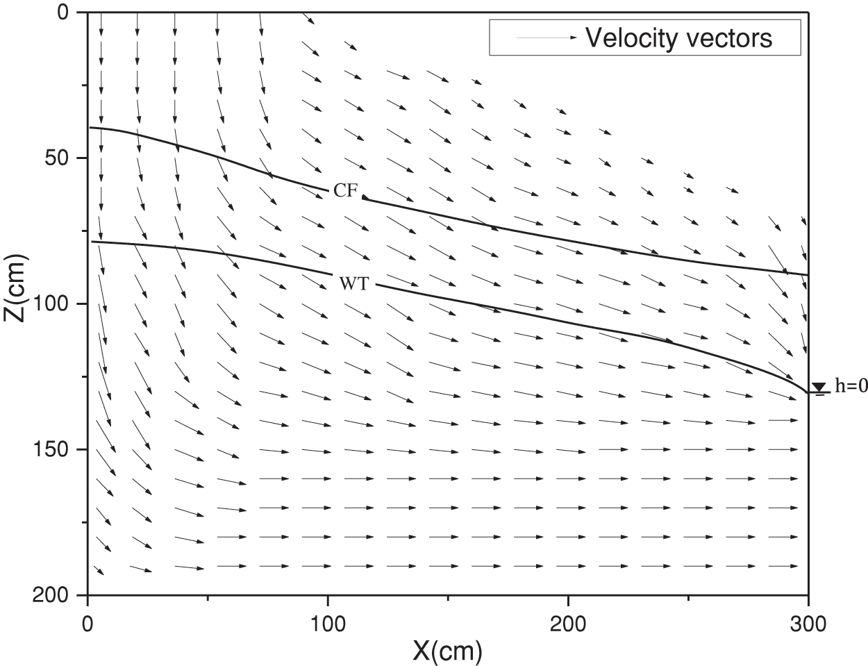
Figure 12: Simulated flow vectors and capillary fringe limits
The behavior of vectors within the capillary fringe can be delineated into three distinct zones:
• The initial zone, spanning from 0 to 50 cm beneath the infiltration band, is characterized by predominant vertical flow.
• The middle zone exhibits significantly greater horizontal flow than vertical flow.
• The last zone, near the exit (285–300 cm), demonstrates entirely vertical flow above the water table (refer to Fig. 12).
Notably, within the middle zone, the horizontal component of the velocity vectors increases notably from the upper limit of the capillary fringe towards the groundwater level, expanding approximately two to fourfold. Numerical findings emphasize the significance of horizontal velocity within the capillary fringe, comparable in importance to the saturated zone. Hence, studies concerning contaminant transport should encompass the consideration of horizontal movement within the capillary fringe, extending beyond conventional limitations confined to the saturated zone.
4.6 Reverse Wieringermeer Effects
The Wieringermeer effect has been documented in a variety of settings, having been first noticed in the Wieringermeer polder in Holland. This phenomena is characterized by a sharp drop in the aquifer’s water level and quick variation in its level. On the other hand, when the capillary fringe becomes closer to the surface, the aquifer rises quickly, which is an inverted manifestation. Reference [15] indicates that when the initial water table is shallow, even a small amount of rainfall infiltration induces a rapid and substantial rise in the water table due to the influence of the capillary fringe. Conversely, when the initial water table equals the riverbed elevation, a shift in groundwater flow patterns occurs following rainfall infiltration. Initially, a groundwater divide and two opposing local flow systems emerge: one directing flow to the upslope unsaturated zone, and the other towards the river. As rainfall persists, the groundwater divide gradually moves upslope, eventually dissipating and forming a stable co-directional regional flow system.
As well examined by [34], this phenomenon vividly demonstrates that even a minor increase in surface water, be it from rainfall or irrigation, triggers a rapid and disproportionate reaction in the water table. The study conducted by Deng et al. [35] in Colorado delved deeper into this phenomenon, emphasizing the tendency to underestimate groundwater elevation in shallow water systems. Their study established a robust correlation between the reverse Wieringermeer effect and rainfall, shedding light on the significant influence of external factors on these hydrological fluctuations. Fig. 13 illustrates the correlation between water table elevation and the upper limit of the capillary fringe, considering both elevation and input flux. As expected, an augmentation in flow corresponds to a rise in the water table level. Notably, as the surface is approached, the elevation of the upper limit of the capillary fringe intensifies. Observably, the length of the capillary fringe exhibits a disproportional increase in response to the amplified flow (from q0 to q1) at the infiltration band, expanding by 3cm. The discrepancy in the length of the capillary fringe depicted in Fig. 13 (a2) and (b2) is attributed to variations in the outlet elevation.
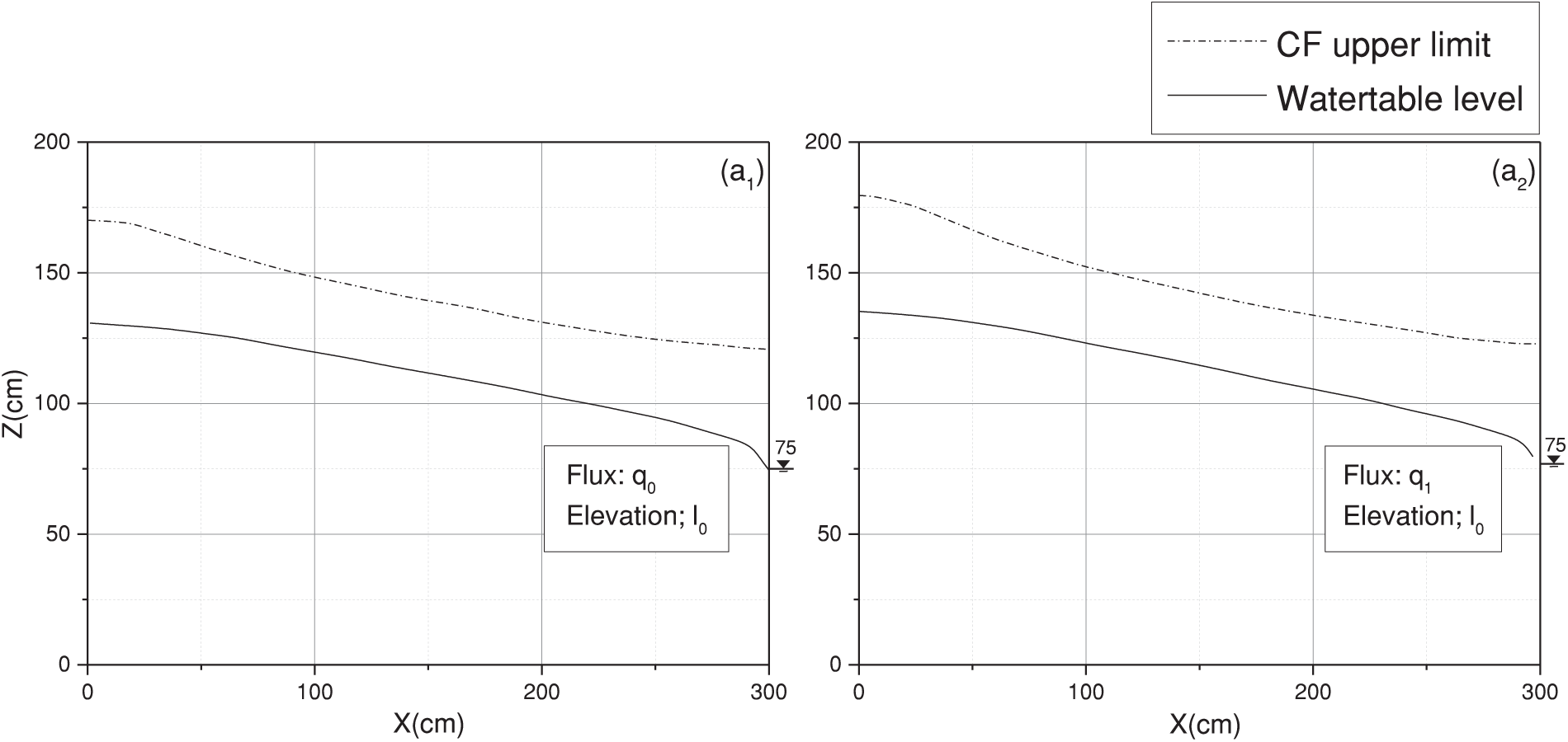

Figure 13: Simulated reverse Wieringermeer effect
To simulate water flow within variably saturated zones, incorporating the capillary fringe, we implemented a mathematical formulation that unifies these three regions into a cohesive continuum. Hydrological investigations employing the potential method have garnered comparatively less attention when juxtaposed with head and pressure methods. However, as demonstrated in this study, focusing on the potential form of the Richards equation remains pertinent and worthwhile. The amalgamation of discharge potential and Kirchhoff potential proves effective in delineating groundwater dynamics.
The numerical solution, employing the finite element method, maintains stability throughout simulations. These simulations underwent validation using experimental data derived from soils falling within the Gardner class. Furthermore, the model offers qualitative predictions of steady-state water table levels and upper limits of the capillary fringe.
The primary achievement of this study lies in precisely delineating the contours of the capillary fringe and seamlessly integrating it into the unsaturated-saturated continuum. Overall, the model demonstrates its capability to accurately simulate hydraulic dynamics within groundwater systems.
The results emphasize the significance of horizontal velocities within the capillary fringe, a key determinant affecting particle migration and transport phenomena. Neglecting the impact of the capillary fringe on hydrology and solute transport could result in misconceptions due to its complex nature and gradient fluctuations. Developing an alternative solution method capable of analyzing the capillary fringe’s dynamics in transient and three-dimensional scenarios is essential, especially when considering various soil permeability models such as van Genuchten or Brooks-Corey. The challenge of non-invasive pressure data collection in field-scale capillary fringe investigations remains a significant hurdle that needs resolution. Further exploration is warranted, particularly in heterogeneous soil conditions and variable water table scenarios. Exciting advancements in hydrogeology await by leveraging novel approaches to model the capillary fringe and porous media, taking inspiration from innovative technologies like neural networks and the groundbreaking contributions of researchers such as [5]. As a prospective avenue of inquiry, our study will delve into the ramifications of elevated capillary fringe levels on construction practices, focusing particularly on the Imperial Valley of California. The significance of capillary fringe effects on construction cannot be understated. In regions characterized by elevated groundwater tables or heightened moisture content, the capillary fringe has the potential to infiltrate porous materials such as soil or concrete. Inadequate safeguards or design measures to counteract capillary rise may result in the upward migration of moisture through concrete, thereby precipitating potential issues such as the corrosion of embedded steel reinforcement (rebar). Employing appropriate rebar placement strategies and protective coatings stands poised as crucial measures to mitigate these risks effectively.
Acknowledgement: We extend our sincere gratitude to Dr. Mustapha Hachimi for his invaluable assistance and unwavering support throughout this research endeavor.
Funding Statement: The authors received no specific funding for this study.
Author Contributions: The authors confirm their contribution to the paper as follows: study conception and design: R. K, A. M; data collection: R. K; analysis and interpretation of results: R. K, A. M; draft manuscript preparation: R. K, A. M. All authors reviewed the results and approved the final version of the manuscript.
Availability of Data and Materials: All the data used in the study is included in the manuscript.
Conflicts of Interest: The authors declare that they have no conflicts of interest to report regarding the present study.
References
1. Xiao Y, Zhu Y. Study of the water vertical infiltration path in unsaturated soil based on a variational method: application of power function distribution of D(θ). Hydrol Sci J. 2022;67(15):2254–61. [Google Scholar]
2. Abdul AS, Gillham RW. Field studies of the effects of the capillary fringe on streamflow generation. J Hydrol. 1989;112(1–2):1–18. [Google Scholar]
3. Cloke HL, Anderson MG, McDonnell JJ, Renaud JP. Using numerical modelling to evaluate the capillary fringe groundwater ridging hypothesis of streamflow generation. J Hydrol. 2006;316(1–4):141–62. [Google Scholar]
4. Zheng Y, Yang M, Liu H. The effects of capillary fringe on solitary wave induced groundwater dynamics. Coast Eng. 2022;177:104202. [Google Scholar]
5. Ronen D, Scher H, Blunt M. On the structure and flow processes in the capillary fringe of phreatic aquifers. Transp Porous Media. 1997;48(1):159–80. [Google Scholar]
6. Silliman BSE. Fluid flow and solute migration within the capillary fringe. Ground Water. 2002;40(1):76–84. [Google Scholar] [PubMed]
7. Nordbotten JM, Dahle HK. Impact of the capillary fringe in vertically integrated models for CO2 storage. Water Resour Res. 2011;47(2):2009WR008958. [Google Scholar]
8. Das TK, Han Z. PFAS release from the subsurface and capillary fringe during managed aquifer recharge. Environ Pollut. 2024;343(1):123166. [Google Scholar] [PubMed]
9. Hack N, Reinwand C, Abbt-Braun G, Horn H, Frimmel FH. Biodegradation of phenol, salicylic acid, benzenesulfonic acid, and iomeprol by Pseudomonas fluorescens in the capillary fringe. J Contam Hydrol. 2015;183(1):40–54. [Google Scholar] [PubMed]
10. Zhang Z, Furman A. Redox dynamics at a dynamic capillary fringe for nitrogen cycling in a sandy column. J Hydrol. 2021;603:126899. [Google Scholar]
11. Guo Y, Zhang S, Gustave W, Liu H, Cai Y, Wei Y, et al. Dynamics of cadmium and arsenic at the capillary fringe of paddy soils: a microcosm study based on high-resolution porewater analysis. Soil Environ Health. 2024;2(1):100057. [Google Scholar]
12. Haberer CM, Rolle M, Cirpka OA, Grathwohl P. Impact of heterogeneity on oxygen transfer in a fluctuating capillary fringe. Groundwater. 2015;53(1):57–70. [Google Scholar]
13. Youngs EG. Effect of the capillary fringe on steady-state water tables in drained lands. J Irrig Drain Eng. 2012;138(9):809–14. [Google Scholar]
14. Alazaiza MYD, Al Maskari T, Albahansawi A, Amr SSA, Abushammala MFM, Aburas M. Diesel migration and distribution in capillary fringe using different spill volumes via image analysis. Fluids. 2021;6(5):189. [Google Scholar]
15. Sun R, Xiao W, Jiang L, Chen Y, Ma Q. Laboratory studies of the temporal evolution process of the riparian groundwater flow system related to rainfall. J Hydrol. 2023;625:130086. [Google Scholar]
16. Bakker M, Nieber JL. Two-dimensional steady unsaturated flow through embedded elliptical layers. Water Resour Res. 2004;40(12):2004WR003295. [Google Scholar]
17. Wen T, Shao L, Guo X. Permeability function for unsaturated soil. Eur J Environ Civ Eng. 2021;25(1):60–72. [Google Scholar]
18. Rucker DF, Warrick AW, Ferré TPA. Parameter equivalence for the gardner and van genuchten soil hydraulic conductivity functions for steady vertical flow with inclusions. Adv Water Resour. 2005;28(7):689–99. [Google Scholar]
19. Dolean V, Hecht F, Jolivet P, Nataf F, Tournier PH. Recent advances in adaptive coarse spaces and availability in open source libraries. Maths In Action. 2022;11(1):61–71. [Google Scholar]
20. Maslouhi A, Lemacha H, Razack M. Modelling of water flow and solute transport in saturated–unsaturated media using a self adapting mesh. IAHS Publ. 2009;331:480. [Google Scholar]
21. Qanza H, Maslouhi A, Abboudi S, Mustapha H, Hmimou A. Unsaturated soil hydraulic properties identification using numerical inversion and in-situ experiments from mnasra area Morocco. KSCE J Civ Eng. 2019;23(11):4949–59. [Google Scholar]
22. Qanza H, Maslouhi A, Hachimi M, Hmimou A. Inverse estimation of the hydrodispersive properties of unsaturated soil using complex-variable-differentiation method under field experiments conditions. Eurasian Soil Sci. 2018;51(10):1229–39. [Google Scholar]
23. Nguyen VH, Hoang VH, Pham VD. Moisture transfer finite element modeling with soil-water characteristic curve-based parameters and its application to Nhan Co red mud basin slope. VNU J Sci: Earth and Env Sci. 2021;37(1):103–15. [Google Scholar]
24. Philip JR. Theory of infiltration. Advan Hydrosci. 1969;5:215–96. [Google Scholar]
25. Berardi M, Difonzo FV. A quadrature-based scheme for numerical solutions to Kirchhoff transformed Richards’ equation. J Comput Dyn. 2022;9(2):69–84. [Google Scholar]
26. Luthin JN, Miller RD. Pressure distribution in soil columns draining into the atmosphere. Soil Sci Soc Am J. 1953;17:329–33. [Google Scholar]
27. Wong S, Craig JR. Series solutions for flow in stratified aquifers with natural geometry. Adv Water Resour. 2010;33(1):48–54. [Google Scholar]
28. Kacimov A, Al-Maktoumi A, Al-Ismaily S, Al-Mayahi A, Al-Shukaili A, Obnosov Y, et al. Water table rise in arid urban area soils due to evaporation impedance and its mitigation by intelligently designed capillary chimney siphons. Environ Earth Sci. 2021;80(17):611. [Google Scholar]
29. Philip JR. Steady infiltration from circular cylindrical cavities. Soil Sci Soc Am J. 1984;48(2):270–8. [Google Scholar]
30. Ameli AA, Craig JR, Wong S. Series solutions for saturated-unsaturated flow in multi-layer unconfined aquifers. Adv Water Resour. 2013;60:24–33. [Google Scholar]
31. Galiullina NE, Khramchenkov MG, Usmanov RM. Mathematical modeling of unsaturated filtration in swelling soils using the capillary-rise problem as an example. J Eng Phys Thermophys. 2021;94:1519–25. [Google Scholar]
32. Loague K, Green RE. Statistical and graphical methods for evaluating solute transport models: overview and application. J Contam Hydrol. 1991;7(1–2):51–73. [Google Scholar]
33. Puy A, Roy PT, Saltelli A. Discrepancy measures for global sensitivity analysis. Technometrics. 2024;71(12):1–9. [Google Scholar]
34. Zhu Y, Ishikawa T, Subramanian SS. Simulation of runoff and infiltration using iterative cross-coupled surface and subsurface flows. Japanese Geotech Soc Spec Publ. 2020;8(3):41–6. [Google Scholar]
35. Deng C, Bailey RT. Assessing causes and identifying solutions for high groundwater levels in a highly managed irrigated region. Agric Water Manag. 2020;240:106329. [Google Scholar]
Cite This Article
 Copyright © 2024 The Author(s). Published by Tech Science Press.
This work is licensed under a Creative Commons Attribution 4.0 International License , which permits unrestricted use, distribution, and reproduction in any medium, provided the original work is properly cited.
 Downloads
 Citation Tools