
 Submit a Paper
 Propose a Special lssue
 Open Access
ARTICLE
Numerical Simulation of Thermocapillary Convection with Evaporation Induced by Boundary Heating
1 Altai State University, Institute of Mathematics and Information Technologies, Barnaul, 656049, Russia
2 Institute of Computational Modelling SB RAS, Department of Differential Equations of Mechanics, Krasnoyarsk, 660036, Russia
* Corresponding Author: V. B. Bekezhanova. Email:
(This article belongs to the Special Issue: Advanced Problems in Fluid Mechanics)
Fluid Dynamics & Materials Processing 2024, 20(7), 1667-1686. https://doi.org/10.32604/fdmp.2024.047959
Received 23 November 2023; Accepted 12 March 2024; Issue published 23 July 2024
 View Full Text
 Download PDF
Abstract
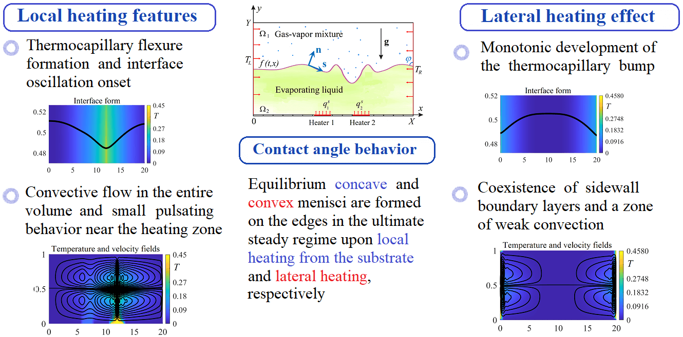
The dynamics of a bilayer system filling a rectangular cuvette subjected to external heating is studied. The influence of two types of thermal exposure on the flow pattern and on the dynamic contact angle is analyzed. In particular, the cases of local heating from below and distributed thermal load from the lateral walls are considered. The simulation is carried out within the frame of a two-sided evaporative convection model based on the Boussinesq approximation. A benzine–air system is considered as reference system. The variation in time of the contact angle is described for both heating modes. Under lateral heating, near-wall boundary layers emerge together with strong convection, whereas the local thermal load from the lower wall results in the formation of multicellular motion in the entire volume of the fluids and the appearance of transition regimes followed by a steady-state mode. The results of the present study can aid the design of equipment for thermal coating or drying and the development of methods for the formation of patterns with required structure and morphology.Graphic Abstract
Keywords
Nomenclature
| C | Concentration (mass fraction of volatile component) |
| Ca | Capillary number |
| D | Vapor diffusion coefficient |
| f | Interface parametrization function |
| F | Auxiliary function in the boundary conditions |
| | Evaporation number |
| Ga | Galilei number |
| Gr | Grashof number |
| g | Gravity acceleration vector |
| h | Fluid layer thickness |
| k | Thermal conductivity coefficient |
| L | Latent heat of vaporization |
| n | Unit normal vector at the interface |
| M | Evaporation mass flow rate |
| Ma | Marangoni number |
| Pr | Prandtl number |
| Pe | Diffusive Peclet number |
| q | Heater temperature |
| Q | Domain of the substrate with the embedded thermal element |
| R | Interface curvature radius |
| | Universal gas constant |
| Re | Reynolds number |
| s | Unit tangent vector on interface |
| t | Time variable |
| T | Temperature |
| | Auxiliary function |
| v | Velocity vector |
| (x, y) | Cartesian coordinates |
| X | Cuvette length |
| Y | Cuvette height |
| Greek Symbols | |
| | Dufour coefficient |
| | Soret coefficient |
| | Thermal expansion coefficient |
| | Concentration expansion coefficient |
| | Kronecker delta |
| | Dimensional coefficient in the boundary condition for the vapor concentration at the interface |
| | Molar mass of the evaporating liquid |
| | Kinematic viscosity coefficient |
| | Density |
| | Surface tension |
| | Temperature coefficient of the surface tension |
| | Thermal diffusivity coefficient |
| | Stream function |
| | Vorticity function |
| | Flow domain |
| | Analogues for the spatial coordinates in the numerical model |
| Subscripts and Superscripts | |
| 0 | Reference flow parameters (specified at |
| j | Denotes belonging to the upper ( |
| l | Integer-valued index, denotes the order number |
| n | Related to the normal vector |
| s | Related to the substrate or to the tangential vector |
| * | Denotes the characteristic values or dimensional quantities |
Thermocapillary convection is a subject of extensive research due to the great importance of the results which can be applied in developing various technologies in the fields of materials science and microfluidic systems. The mechanism of occurrence of convective motion is related to changes in the surface tension of a liquid. The changes can result from an external thermal action [1,2], concentration effects [3–5] or evaporation [6–8] on the liquid surface. If the combined action of these effects occurs, they can be amplified or they can compete with each other, causing the alteration of flow regimes and instabilities of different nature. The control of thermally induced and/or concentration-induced motion and the dynamical operation of transport processes in the volume of a liquid with a free surface or in multicomponent systems with interfaces are crucial for the development of new innovative approaches in material engineering and various smart technologies. These include coating technologies connected with obtaining coversheets with given functional characteristics [4,9–11], methods applied upon surface purification [5,12,13], bioengineering and medical technologies, including microfluidic sorting [14,15], targeted drug delivery [16] and local elevation/reduction of components in fluid solutions [2,17], as well as various approaches directed towards the enhancement of heat transfer characteristics in electronic devices [18].
Fluidic systems with working media being in different aggregate states and filling domains with outer solid boundaries as well as limited volumes of the liquid contacting with a rigid substrate have a three-phase contact line near which the convection characteristics can also significantly vary [19,20]. The development of mathematical models based on the conservation laws of mass, momentum and energy for describing the fluid dynamics in domains with solid walls and internal interfaces is fraught with difficulties. The main challenges are in choosing a way to describe the three-phase line motion (or three-phase points for two-dimensional statements), correct determining the dynamic contact angle, and substantiating the kinematic compatibility of the boundary conditions of different types for the velocity function [21–24]. The problem still has no well-posed closure. For the first time, this inconsistency between the conditions on the free surface and the no-slip ones in the contact point neighborhood was pointed out in [21] and was mathematically proved in [22] with minimal assumptions for the velocity and free surface smoothness. In the common case, the energetic norm of the velocity field will become infinite which means that the energy becomes unbounded. There are various approaches to correctly formulate mathematical models for describing flows of a viscous incompressible liquid with a moving contact line or a moving contact point in the two-dimensional statement. The approaches allow one to replace the no-slip conditions with the slip conditions on the solid wall sections near the contact line, or the asymptotic approach can be used; in addition, one can also consider the suggestion about the contact angle being equal to π in the leakage regime or to “zero” in the runoff one as well as other statements. The solvability of the initial boundary-value problems was studied for a number of mathematical models of fluid flows with dynamic contact angles [23–25]. The well-posedness of the statement with the free boundary and dynamic contact angle was proved in [24,25] in the case when the no-slip condition on the solid boundary was changed to the condition of proportionality of tangential stresses to tangential velocities. The existence of a solution and asymptotic expansion in the neighborhood of the contact point were proved, and the regularity of the free boundary was shown in the statement with a uniformly moving contact point. Two-dimensional and axis-symmetric stationary problems were studied in [23] in the case of capillary numbers being small. Theoretical results of the study of apparent contact angles in a problem of an evaporating liquid placed on a solid substrate are presented in [26]. In [27], a moving contact line problem for two-phase incompressible flows was investigated based on the kinematic approach using an evolution equation for the contact angle in terms of the transporting velocity field; this approach and other common models including the gradients of surface tension and mass transfer across the fluid–fluid interface were analyzed. The behavior of the contact angle relative to the contact point velocity was investigated in physical experiments (see [28] and papers cited there). In [28], the numerical investigations of isothermal fluid flows with the dynamic contact angle were carried out for a problem with the proportionality conditions of tangential stresses and velocities on solid walls; here, rather good agreement with experimental results was confirmed and the monotonous character of the dependence of the contact angle on the contact point velocity was shown. In [29], this problem was studied in terms of the influence of the thermal boundary regimes on the contact point velocity. The thorough consideration of the statements in terms of contact lines is due to the problems of heat transfer processes in fluids, especially, in the case of evaporation [20,30]. The evaporation rate and heat flux density in the vicinity of the contact lines are very high [31]. The value of the contact angle depends on the temperature of the heated solid surface and on the evaporation rate as well as on the contact line velocity. One of the effects observed experimentally is the contact angle hysteresis. The effect consists in the existing difference between the advancing and receding contact angles [32] (see review in [20] and references in [20,32]). This phenomenon is studied based on different approaches in a significant number of papers. An ambiguity appears even in the definition of the static value of the contact angle. Experiments on wetting dynamics allow one to investigate various problems of the contact line motion concerning the surface heterogeneities. On a small scale, they lead to contact line deformation while on a macroscopic scale, they result in contact angle hysteresis.
In the present paper, we study the structure and characteristics of convective regimes in a liquid–gas system under diffusive-type evaporation based on numerical modeling. We investigate the influence of different types of thermal action on the flow structure, behavior of the phase boundary and dynamic contact angle. We consider the cases of local heating from the substrate and distributed lateral thermal impact. The simulation is carried out in the framework of a two-dimensional mathematical model whose implementation admits the correct agreement between the no-slip boundary condition and the moving contact points [21,33].
2.1 Basic Assumptions and Description of the Physical System
We investigate joint non-stationary flows in a two-layer system filling a plane rectangular cuvette (Fig. 1). The domains Ω1 and Ω2 are occupied by gas and liquid media, respectively, and divided by a common interface which is a thermocapillary surface admitting the mass transfer of the diffusive type due to evaporation/condensation. The phase boundary is considered as a smooth curve embedded in two-dimensional space. The curve is defined by the equation
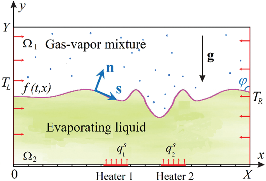
Figure 1: The scheme of a two-phase flow in the Cartesian coordinates
Initially, both fluids are at rest, and the interface is straight so that the left and right contact angles φ are equal to 90°. The media are in the state of intermutual saturation with the average concentration vapor in the gas
We assume that the system is in the terrestrial gravity field
To model the convective heat and mass transfer in the domains Ωj, we use the governing equations written in
Assuming that the vapor is a passive admixture which does not change any properties of the background gas, we add the convection-diffusion equation
to model the process of vapor transfer in the gas. The subscripts
2.3 Initial and Boundary Conditions
The following conditions define the initial state of the system at the time moment
The initial location of the interface is set by the equation
On the outer boundary ∂Ω the conditions for the stream functions
Here,
The interface conditions are derived on the basis of the conservation laws for mass, momentum and energy, while other ones are the result of using additional suppositions with regard to the character of the processes under study [7,34]. In the problem being discussed, the basic assumptions are the following:
(i) the thermocapillary surface
(ii) we consider that
Then, complementing the kinematic, dynamic and energy conditions with the standard continuity conditions for the velocity and temperature and the relation for the vapor concentration on the phase boundary, we can write the interface conditions at
Here,
The sign of M determines the regime of the phase transitions. If
A detailed substantiation of the problem statement presented is given in [33]. Therein, the consistent interpretation of the three-phase contact points in the physical system is explained in accordance with the conception imposed in [21], where the idea of the kinematic compatibility of the no-slip condition and moving three-phase contact point was convincingly justified in terms of the displacing and displaced fluids.
3 Results of Numerical Modeling
3.1 Brief Remarks on the Numerical Algorithm and Calculation Parameters
We use the numerical algorithm proposed in [33] in order to solve problem (1)–(5). A distinctive peculiarity of the method is that in its implementation there is no need to explicitly keep track of the location of the contact points. The algorithm provides calculations in the canonic computation region
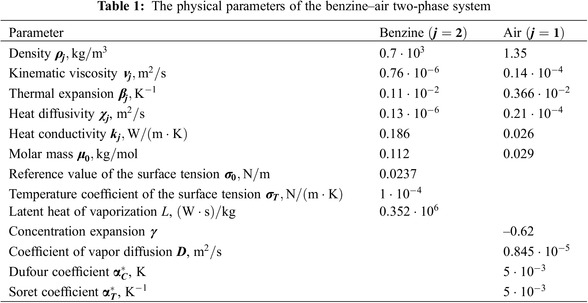
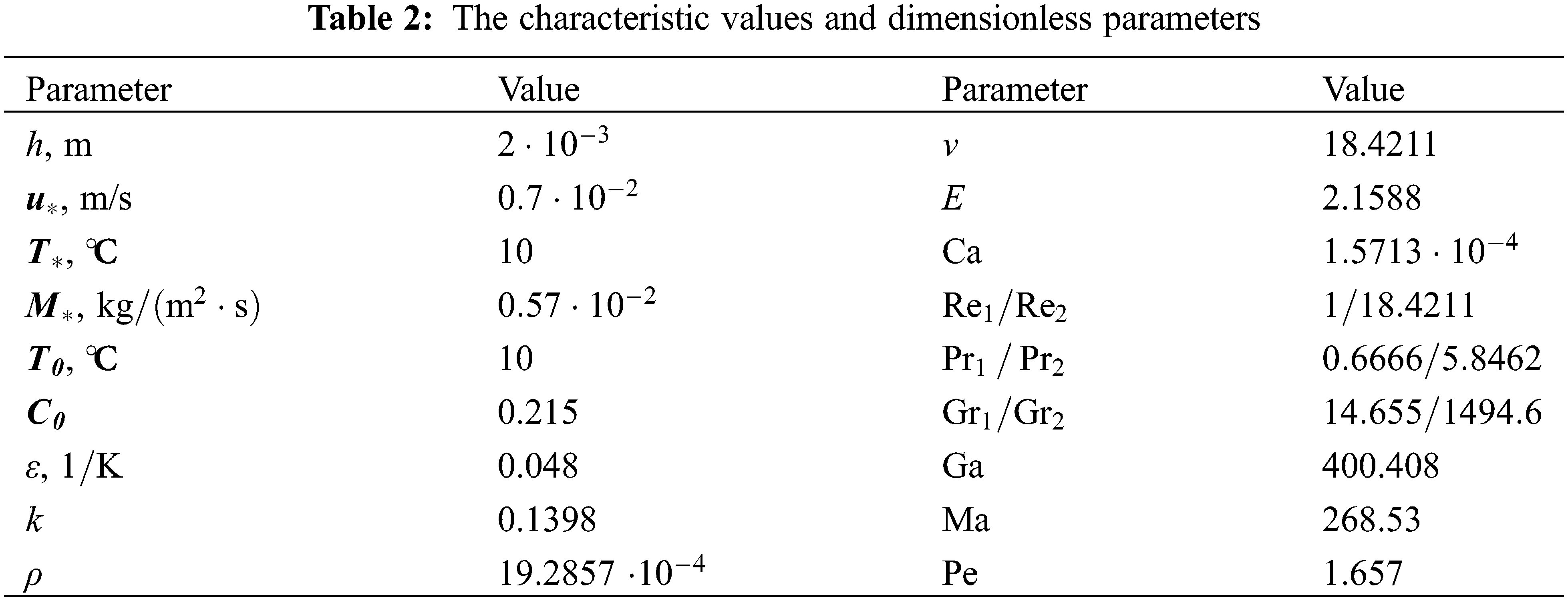
The dynamics of convective heat and mass transfer in a closed cuvette filled with the liquid and gas media divided by an interface under various heating conditions is studied on the example of a benzene–air system. The physicochemical parameters of the working fluids are given in Table 1 [35,36]. The geometrical characteristics of the system are chosen as follows: the cuvette length and height are
We consider the cases of non-stationary heating from below (Heating mode I) and from the side of the lateral walls (Heating mode II). In Heating mode I, the temperature of the lateral walls does not change,
Figs. 2–6 demonstrate the evolution of the basic characteristics of the bilayer system upon local non-stationary heating. We present the parameters of the system at certain time moments in order to show the qualitative alteration of the flow pattern accompanied by the formation of typical transition regimes (Figs. 2–5) as well as the ultimate mode (Fig. 6) which are realized in the system heated from below.
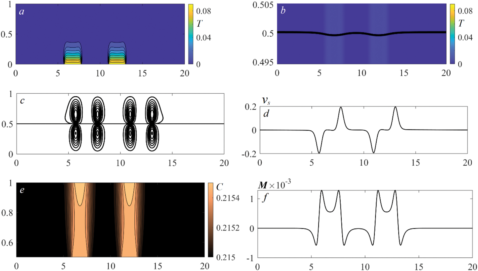
Figure 2: The characteristics of the benzine–air system 2.5 s after switching on the bottom heaters: temperature distributions and isotherms (a); temperature distributions near the interface and interface shape, the formation of thermocapillary flexures in the zones of thermal impact (b); velocity field, the appearance of double-vortex motion above the heaters (c); tangential velocity
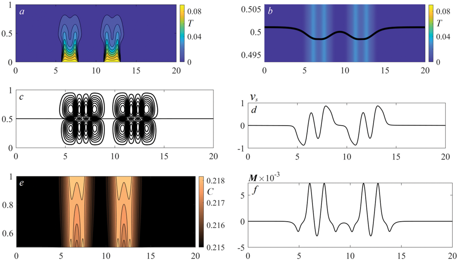
Figure 3: The characteristics of the benzine–air system 5 s after switching on the bottom heaters: temperature distributions and isotherms (a); temperature distributions near the interface and interface shape, the thermocapillary-driven dimples (b); velocity field, the transition to the multicellular regime upon heating (c); tangential velocity
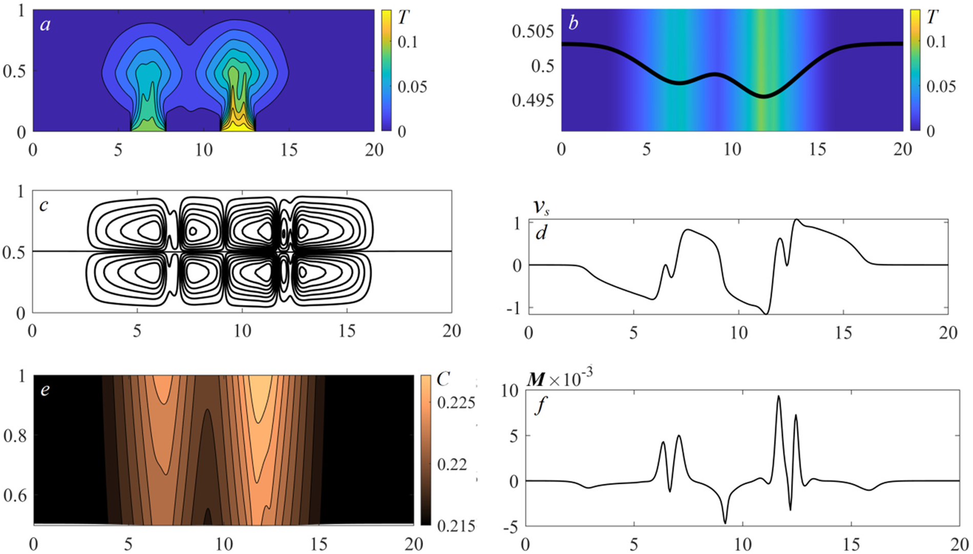
Figure 4: The characteristics of the benzine–air system 15 s after switching on the bottom heaters: temperature distributions and isotherms (a); temperature distributions near the interface and interface shape, marked changes in the interface curvature accompanied by the wave behavior of the surface (b); velocity field, the reverse transition to double-vortex motion in the domains of local heating (c); tangential velocity
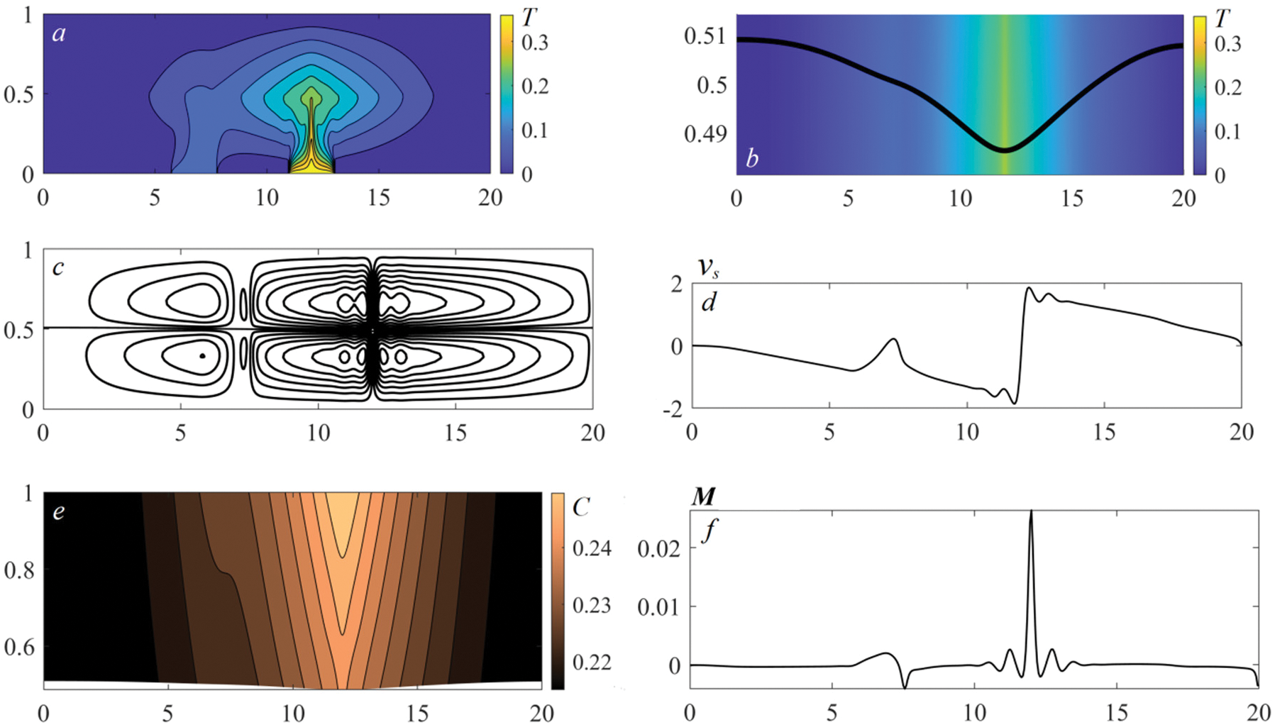
Figure 5: The characteristics of the benzine–air system 64 s after switching on the bottom heaters: temperature distributions and isotherms (a); temperature distributions near the interface and interface shape, the decay of the thermocapillary dimple above “weak” Heater 1 (b); velocity field, the degeneration of the multicellular regime (c); tangential velocity
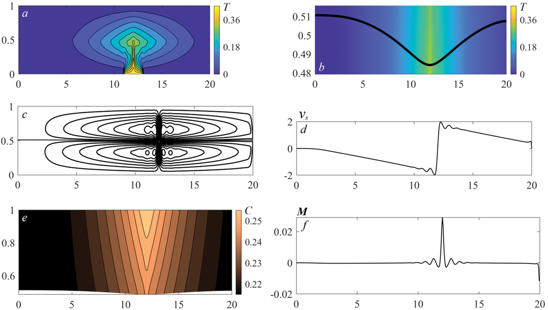
Figure 6: The characteristics of the ultimate convective regime in the benzine–air system 200 s after switching on the bottom heaters: temperature distributions and isotherms (a); temperature distributions near the interface and interface shape, the stable thermocapillary flexure in the heating zone (b); velocity field, the eventual dual-vortex regime (c); tangential velocity
We note that the convective mechanism completely defines the flow structure and character of changes in the basic characteristics. The heat transfer from the thermal elements triggers cascade responses affecting the system dynamics. The onset of motion is caused by the buoyancy force; here, the topological pattern of the flow is determined by the number and size of the heaters. The quantity of vortices forming typical convective cells at the first stage is equal to 2n, where n is the number of thermal elements. All the swirls have pairwise opposite circulation. Ascendant currents transferring heat to the interface are formed in the domains of thermal impact directly above the thermal elements. The velocity of rising convective flows is much higher than the velocity of the diffusive transfer in any direction (this is indicated by the structures of temperature and velocity fields in Figs. 2a, 2c). Once the heat reaches the interface, there appear surface effects. The surface tension of the liquid changes and the interface is distorted (Fig. 2b). The motion of the liquid along the interface occurs due to the action of the Marangoni force (the tangential velocity
The initial convective regime is replaced by a multicellular mode whose characteristics are shown in Fig. 3. The new state also represents a transient mode which is characterized by a more complex flow structure with a higher velocity of motion (compare the values of
The jump-like change in the temperature of Heater 2 leads to the development of oscillatory regimes with the behavior of the system characterized by the oscillations of the basic parameters near certain values. The wave behavior of the interface distinguishes these regimes from the first two modes (Fig. 4). The liquid–gas boundary undergoes oscillations, accompanied by periodical irregular variations of the surface curvature over the entire length (Fig. 4b). We observe a gradual transformation of the vortices caused by the temperature difference of the heaters. The quadruple-vortex motion above each thermal element degenerates into a two-fold one; here, the cells above the hotter heater have several deformed cores with more intensive motion (Figs. 4c, 4d). It explains the higher evaporation rate in the action zone of the second heater (Fig. 4f). The “fork” structure of the concentration field in the gas phase is typical for this mode (Fig. 4e). This oscillatory regime is also a transient one. With time it evolves into the next mode in which the oscillatory behavior of all the characteristics persists. Strong heating under the exposure to Heater 2 attenuates the surface tension of the interface and it becomes cambered (Fig. 5b) and continues to oscillate. Every change-over of Heater 2 results in a decrease in the liquid thickness in the zone of the thermal impact. Therefore, the velocity of convective rising flows grows. It entails an increase in the velocity of thermocapillary spreading and intensification of evaporation (Figs. 5d, 5f). The “club-shaped” concentration structure followed by the “fork” pattern is preserved in the gas phase (Fig. 5e).
After switching off Heater 1, the double-vortex motion in each fluid is settled. The flow occupies almost the entire cuvette. There is one zone with an ascendant flow above Heater 2 (Fig. 6c), where the maximum evaporation rate is reached (Fig. 6f). The typical thermocapillary flexure persists here (Fig. 6b). We note that the most intensive vapor condensation occurs in the vicinity of the lateral wall near the operating heater. The whole interface continues to oscillate at a certain finite frequency, but the pronounced surface waves propagating from the heating zone to the periphery vanish. The regime is ultimate; here, the maximum values of the flow velocity and evaporation rate also oscillate near certain values. The oscillatory character of convection is induced by the first abrupt change in the temperature of Heater 2, and it is retained even when the intensity of thermal load stops changing. Thus, the principal mechanism which governs the characteristics of the appearing transient and eventual modes is a convective one.
In contrast to the case of local heating from below, the dynamical characteristics as well as the behavior of the liquid–gas interface do not qualitatively change with time upon lateral heating. Figs. 7–9 allow one to track the dynamics of the basic characteristics when the bilayer system undergoes non-stationary lateral heating. One can see that boundary thermal and concentration layers (images (a) and (e) in Figs. 7–9) develop close to the side walls. The structure of the corresponding fields is explained by a slight diffusive transfer in any directions in comparison with the convective transfer. This directly follows from the heat and molecular transport equations. Given the values of the Reynolds and Prandtl numbers for the liquid layer (at
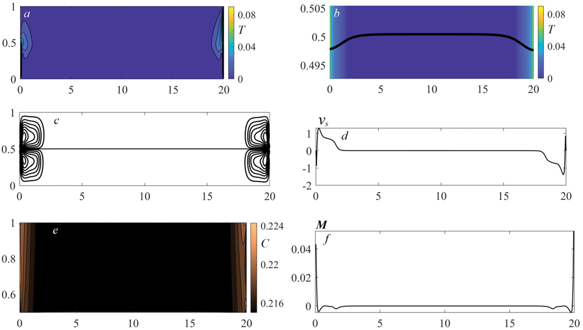
Figure 7: The characteristics of the benzine–air system at
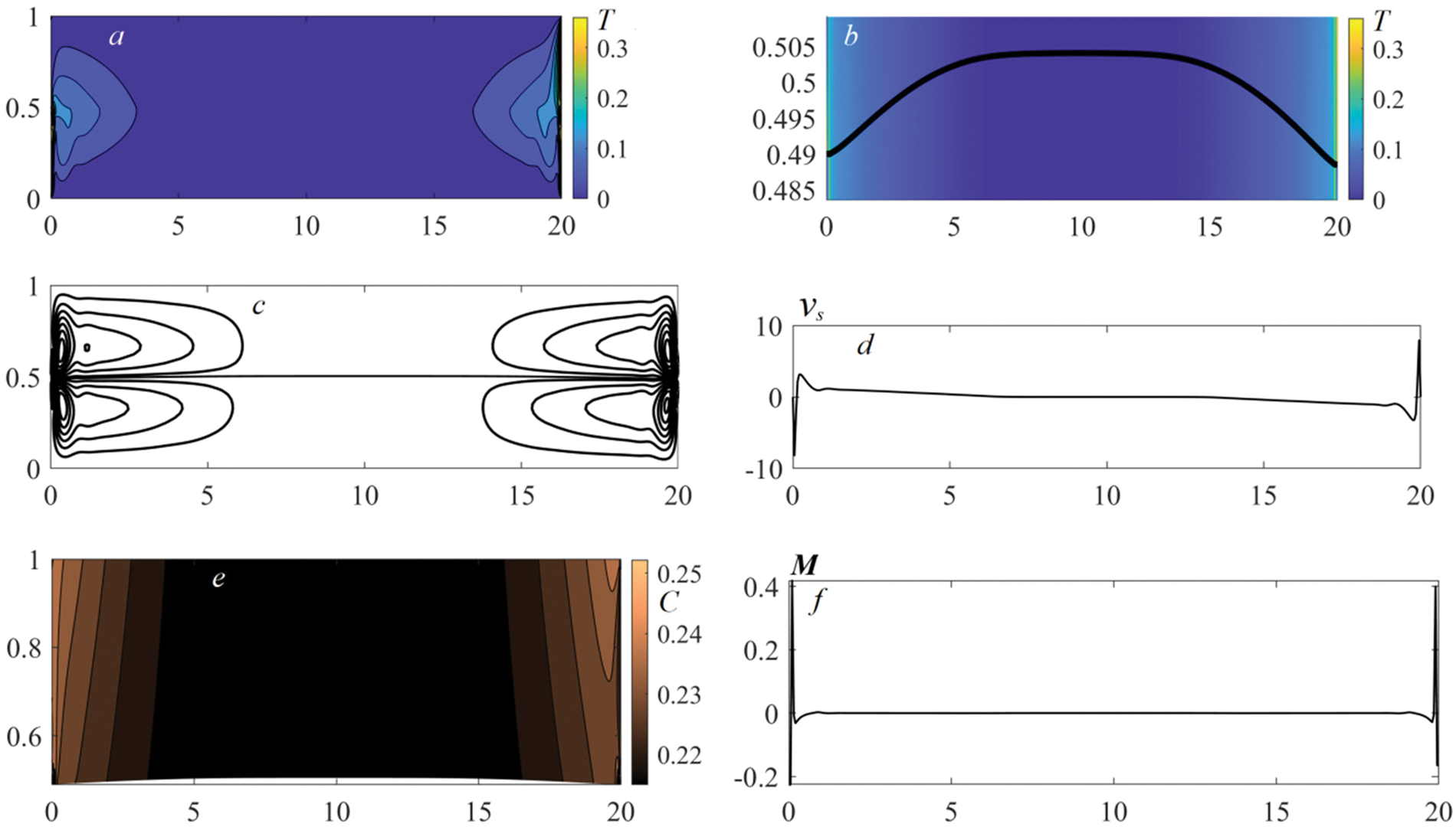
Figure 8: The characteristics of the benzine–air system at
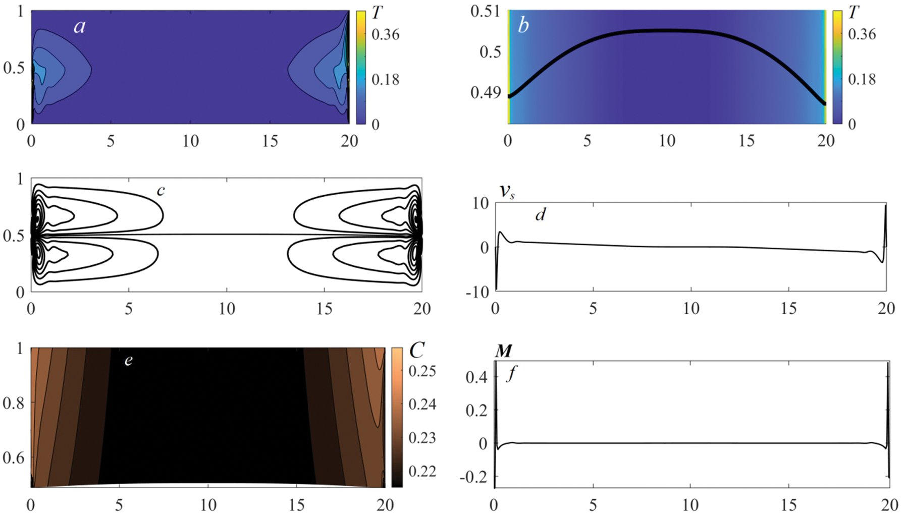
Figure 9: The characteristics of the ultimate convective regime in the benzine–air system at
The specific temperature distribution entails other behavior of the interface. The phase boundary has a convex upward form in response to lateral heating. It results from the combined action of the surface tension forces and arising pressure gradients. The lateral heating attenuates the interface surface tension. At the same time, the pressure from the gas side near the cuvette edges is higher than that from the liquid, and therefore, the phase boundary hangs down therein. Out of the thermal “spots”, the pressure drop vanishes and the interface is forced out upwards. It leads to the formation of a thermocapillary bump. The higher the intensity of the external thermal load, the larger the pressure drop and the larger the height of the interface rise (compare images (b) in Figs. 7–9).
As to the velocity field pattern, we note that the wall swirls near both side boundaries evolve into the vortex structures with a complex symmetry. The eventual flow regime is characterized by the coexistence of pronounced boundary layers with a near-wall core and a slow-convecting zone. Here, the velocity of motion induced by the distributed lateral heating is well above those in the case of the local thermal load from the substrate (compare the values of
3.4 Behavior of the Contact Angle
The behavior of the dynamic contact angle is illustrated by an example of the angle
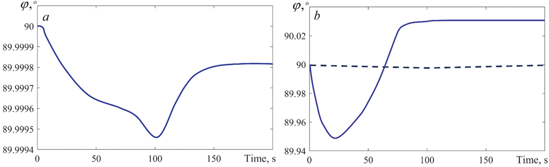
Figure 10: The dynamic contact angle
Another character of the contact angle alterations is observed under lateral heating. The intensive supply of heat from the side walls results in a rapid significant decrease in the
The dynamics of the two-phase system with a deformable interface admitting the mass transfer due to evaporation in the box-shaped cuvette subjected to various heating conditions is investigated at an example of the system of working media like benzine–air. The study is carried out in the framework of a full two-sided model based on the Boussinesq approximation. The original approach used to state the problem in terms of new auxiliary functions allows one to derive the corresponding numerical model that enables one not only to calculate all the system characteristics, including the mass evaporation rate, but also to scrutinize the behavior of the dynamic contact angles, depending on the heating mode.
Based on the numerical simulation, considerable differences in the behavior of the bilayer fluidic system are elucidated. An eventual regime under the local heating from below is established through the transient modes, whereas the inertia of the system behavior is typical for the case of the distributed lateral heating, giving rise to monotonous changes in the hydrodynamic, temperature and concentration characteristics. Here, the amplitudes of the interface deformations under the thermal load applied on the side walls is lower than those under the other type of heating. Two various scenarios of the interface evolution are realized, depending on the type of the external thermal action. A thermocapillary flexure and a thermocapillary bump appear upon heating from the substrate and side walls, respectively. In the first case, convective heat and mass exchange occurs in the whole volume of the fluids, and equilibrium concave menisci are formed on the edges in the ultimate steady regime. The second heating regime leads to the appearance of a boundary layer and near-wall temperature and concentration patterns; here, convex menisci are observed on the heated lateral walls. In both cases, the contact angle variation in time is described by the numerical model.
The results obtained contribute to a better understanding of the interaction of the basic mechanisms governing the convective regimes in systems with internal interfaces and points of three-phase contact. The results of the present study can aid in designing equipment for thermal coating or drying and working sections employed in control tools for various applications as well as in developing methods for the formation of patterns of the required structure and morphology on solid surfaces.
Acknowledgement: The authors express gratitude to Dr. O.M. Lavrenteva for useful discussions.
Funding Statement: The work of O.N. Goncharova was carried out in accordance with the State Assignment of the Russian Ministry of Science and Higher Education entitled “Modern Models of Hydrodynamics for Environmental Management, Industrial Systems and Polar Mechanics”, Govt. Contract Code: FZMW-2024-0003, https://minobrnauki.gov.ru/.
Author Contributions: The authors confirm equal contribution to the paper: study conception and design, data collection, analysis and interpretation of results, draft manuscript preparation: V.B. Bekezhanova. O.N. Goncharova. All authors reviewed the results and approved the final version of the manuscript.
Availability of Data and Materials: All the data are based on publicly available documents, whose data sources were cited in the manuscript.
Conflicts of Interest: The authors declare that they have no conflicts of interest to report regarding the present study.
References
1. Bekezhanova VB, Fliagin VM, Goncharova ON, Ivanova NA, Klyuev DS. Thermocapillary deformations of a two-layer system of liquids under laser beam heating. Int J Multiphas Flow. 2020;132:103429. [Google Scholar]
2. Al-Muzaiqer MA, Kolegov KS, Ivanova NA, Fliagin VM. Nonuniform heating of a substrate in evaporative lithography. Phys Fluids. 2021;33:092101. [Google Scholar]
3. Zuev AL, Kostarev KG. Certain pecularities of solutocapillary convection. Phys-Uspekhi. 2008;51(10):1027–45. [Google Scholar]
4. Farzeena C, Vinay TV, Lekshmi BS, Ragisha CM, Varanakkottu SN. Innovations in exploiting photo-controlled Marangoni flows for soft matter actuations. Soft Matter. 2023;19(28):5223–43. [Google Scholar] [PubMed]
5. Feldmann D, Maduar S, Santer M, Lomadze N, Vinogradova O, Santer S. Manipulation of small particles at solid liquid interface: light driven diffusioosmosis. Sci Rep. 2016;6(1):36443. [Google Scholar] [PubMed]
6. Routh AF, Russel WB. Horizontal drying fronts during solvent evaporation from latex films. American Institute of Chemical Engineers Journal. 1998;44:2088–98. [Google Scholar]
7. Bekezhanova VB, Goncharova ON. Problems of the evaporative convection (review). Fluid Dyn. 2018;53(1):S69–102. [Google Scholar]
8. Kolegov KS, Barash LY. Applying droplets and films in evaporative lithography. Adv Colloid Interfac. 2020;285:102271. [Google Scholar]
9. Prevo BG, Hon EW, Velev OD. Assembly and characterization of colloid-based antireflective coatings on multicrystalline silicon solar cells. J Mater Chem. 2007;17(8):791–9. [Google Scholar]
10. Hatton B, Mishchenko L, Davis S, Sandhage KH, Aizenberg J. Assembly of large-area, highly ordered, crack-free inverse opal films. Proc Natl Acad Sci. 2010;107(23):10354–9. [Google Scholar] [PubMed]
11. Hammond PT. Building biomedical materials layer-by-layer. Mater Today. 2012;15(5):196–206. [Google Scholar]
12. Du F, Felts JR, Xie X, Song J, Li Y, Rosenberger MR, et al. Laser-induced nanoscale thermocapillary flow for purification of aligned arrays of single-walled carbon nanotubes. Am Chem Soc Nano. 2014;8(12):12641–9. [Google Scholar]
13. Ivanova N, Starov VM, Trybala A, Flyagin VM. Removal of micrometer size particles from surfaces using laser-induced thermocapillary flow: experimental results. J Colloid Interface Sci. 2016;473:120–5. [Google Scholar] [PubMed]
14. Chhasatia VH, Sun Y. Interaction of bi-dispersed particles with contact line in an evaporating colloidal drop. Soft Matter. 2011;7(21):10135–43. [Google Scholar]
15. Wyatt Shields CIV, Reyes CD, Lopez GP. Microfluidic cell sorting: a review of the advances in the separation of cells from debulking to rare cell isolation. Lab Chip. 2015;15(5):1230–49. [Google Scholar] [PubMed]
16. Takhistov P, Chang HC. Complex stain morphologies. Ind Eng Chem Res. 2002;41(25):6256–69. [Google Scholar]
17. Al-Muzaiqer MA, Ivanova NA, Fliagin VM, Lebedev-Stepanov PV. Transport and assembling microparticles via Marangoni flows in heating and cooling modes. Colloids Surf A: Physicochem Eng Asp. 2021;621(5):126550. [Google Scholar]
18. Chen L, Wang Y, Qi C, Tang Z, Tian Z. A review of methods based on nanofluids and biomimetic structures for the optimization of heat transfer in electronic devices. Fluid Dyn Mater Process. 2022;18(5):1205–27. doi:https://doi.org/10.32604/fdmp.2022.021200. [Google Scholar] [CrossRef]
19. Helseth LE, Fischer TM. Particle interactions near the contact line in liquid drops. Phys Rev E. 2003;68(4):042601. [Google Scholar]
20. Ajaev VS, Kabov OA. Heat and mass transfer near contact lines on heated surfaces. Int J Heat Mass Tran. 2017;108:918–32. [Google Scholar]
21. Dussan EBV, Davis SH. On the motion of a fluid-fluid interface along a solid surface. J Fluid Mech. 1974;65:71–95. [Google Scholar]
22. Pukhnachov VV, Solonnikov VA. On the problem of dynamic contact angle. J Appl Math Mech. 1982;46(6):771–9. [Google Scholar]
23. Baiocchi C, Pukhnachov VV. Problems with unilateral constrains for the Navier-Stokes equations and the problem of dynamic contact angle. J Appl Mech Tech Phy. 1990;31(2):185–97. [Google Scholar]
24. Kroener D. The flow of a fluid with a free boundary and dynamic contact angle. ZAMM J Appl Mat Mech. 1987;67(5):T304–6. [Google Scholar]
25. Kroener D. Asymptotic expansion for a flow with a dynamic contact angle. In: Heywood J, Masuda K, Rautmann R, Solonnikov VA, editors. The Navier–Stokes Equations: Theory and Numerical Methods. Berlin: Springer; 1990. p. 49–59. [Google Scholar]
26. Rednikov AY, Colinet P. Contact angles for perfectly wetting pure liquids evaporating into air: between de Gennes-type and other classical models. Phys Rev Fluids. 2020;5:114007. [Google Scholar]
27. Fricke M, Marić T, Bothe D. A kinematic evolution equation for the dynamic contact angle and some consequences. Phys D: Nonlinear Phenom. 2019;394:26–43. [Google Scholar]
28. Doerfler W, Goncharova O, Kroener D. Fluid flow with dynamic contactangle: numerical simulation. ZAMM J Appl Math Mech. 2002;82(3):167–76. [Google Scholar]
29. Goncharova ON, Marchuk IV, Zakurdaeva AV. Investigation of behavior of the dynamic contact angle in a problem of convective flows. Eurasian J Math Comput Appl. 2017;5(4):27–42. [Google Scholar]
30. Ajaev VS, Gambaryan-Roisman T, Stephan P. Static and dynamic contact angles of evaporating liquids on heated surfaces. J Colloid Interf Sci. 2010;342:550–8. [Google Scholar]
31. Karchevsky AL, Cheverda VV, Marchuk IV, Gigola TG, Sulyaeva VS, Kabov OA. Heat flux density evaluation in the region of contact line of drop on a sapphire surface using infrared thermography measurements. Microgravity Sci Technol. 2021;33:53. [Google Scholar]
32. Nikolayev VS, Gavrilyuk SL, Gouin H. Modeling of the moving deformed triple contact line: influence of the fluid inertia. J Colloid Interf Sci. 2006;302:605–12. [Google Scholar]
33. Bekezhanova VB, Goncharova ON. Thermodiffusion effects in a two-phase system with the thermocapillary deformable interface exposed to local heating. Int J Multiphas Flow. 2022;152:103429. [Google Scholar]
34. Andreev VK, Gaponenko YA, Goncharova ON, Pukhnachov VV. Mathematical models of convection. Berlin: De Gruyter; 2020. p. 1–432. [Google Scholar]
35. Shliomis MI, Yakushin VI. Convection in a binary system with evaporation. Uchenye Zapiski Permskogo Universiteta. Seriya: Gidrodinamika. 1972;4:129–40 [In Russian]. [Google Scholar]
36. Vargaftik NB. Handbook of thermophysical properties of gases and liquids [In Russian]. Moscow: Nauka; 1972. [Google Scholar]
Cite This Article
 Copyright © 2024 The Author(s). Published by Tech Science Press.
This work is licensed under a Creative Commons Attribution 4.0 International License , which permits unrestricted use, distribution, and reproduction in any medium, provided the original work is properly cited.
 Downloads
 Citation Tools