Numerical Simulation of Oil-Water Two-Phase Flow in Low Permeability Tight Reservoirs Based on Weighted Least Squares Meshless Method

1  Introduction

Low-permeability tight oil and gas reservoirs are critical for oil and gas development due to their rich hydrocarbon reserves, varied reservoir types, and extensive distribution. Within proven reserves, tight oil reservoirs make up over two-thirds of national reserves, showing great development potential. However, tight oil has intricate oil-water (OW) zones, low porosity, and cannot be easily extracted using conventional techniques, posing challenges [1]. Large-scale development of tight reservoirs typically requires horizontal wells and hydraulic fracturing [2,3]. However, during fracturing, fluid readily enters the reservoir. The modified region exhibits higher pore water saturation than bound water saturation due to retained fracturing fluid, original formation water, or water injection to maintain pressure. Thus, OW two-phase flow with complex migration patterns is common in low-permeability tight reservoirs [4,5]. After fracturing, tight reservoirs retain natural fractures but also develop large conductive fractures, significantly altering flow patterns. Understanding OW flow in fractured tight reservoirs is critical for guiding and optimizing production in these reservoirs.

In recent years, scholars have paid considerable attention to and developed numerical simulation of OW two-phase flow in fractured reservoirs. Currently, numerical simulation methods are primarily categorized into two types: continuous medium models and discrete medium models [6]. Continuous medium models mainly include the Equivalent Continuous Medium Model [7] and the Dual Porosity Model [8,9], where fractures and matrix are treated as discretized elements of equal size. In discrete medium models, fractures are handled as (n-1)-dimensional entities in an n-dimensional reservoir, meaning one-dimensional lines in two-dimensional reservoirs and two-dimensional planes in three-dimensional problems. This difference in handling fracture geometry is fundamental between the two methods. Under both models, some scholars employ numerical methods like finite difference method [10,11], finite element method [12], and finite volume method [13] for flow calculations. However, studies on simulating OW two-phase flow in tight reservoirs considering fracture morphology and geology are limited. Reservoir conditions are often complex with intricate boundaries and fractures. Traditional grid-based schemes struggle to represent this complexity, causing large model grids, high computational degrees of freedom, and substantially increased computation time, restricting field application [14,15].

Unlike traditional grid discretization, the meshless method employs nodal discretization of the computational domain, free from grid topology constraints, providing more flexibility in domain representation. Thus, meshless methods offer a convenient approach for modeling complex geometries. Meshless method research traces back to the 1970s, with early techniques like the vortex method [16], generalized finite difference method [17,18], and smooth particle hydrodynamics [19]. However, meshless method application in reservoir simulation has been much less compared to finite volume, finite element, and other methods, with research focused on solid mechanics. Meshless methods have two key advantages over grid-based methods: increased flexibility in domain discretization and higher accuracy in calculating potential fields like pressure and stress. With the same discretization dimension (equal grid/point number), meshless methods can achieve higher precision in solving problems like pressure and stress vs. grid-based methods (e.g., finite volume, finite difference, finite element). This is because grid-based methods are constrained by grid topology and can only approximate derivatives between adjacent grids, while meshless methods use shape functions to approximate within the influence domain, utilizing more nodal information and offering higher theoretical precision.

Some collocation-type meshless methods still require background grids for discretizing integral equations, limiting complex geometry capture. The point interpolation approach is a purely meshless method not needing background grids, offering greater flexibility in discretizing domains with complex geometries unconstrained by grid topology. It ensures computational accuracy while establishing relatively lower degree-of-freedom models more faithful vs. grid-based methods, potentially reducing computational needs while providing accurate physical domain representation. This paper introduces meshless methods to study OW two-phase flow in tight reservoirs, motivated by theoretical advantages in handling actual complex reservoir geometries. General methods like local boundary integral equation [20] and meshless local Petrov-Galerkin [21] using moving least squares for function approximation and meshless discretization do not require background grid integration, improving efficiency. However, their low accuracy and poor stability limit real problem applications. Xiong et al. [22] proposed a weighted least squares (WLS) meshless method improving stability. But moving least squares approximate functions are computationally expensive without the delta function property [23], complicating essential boundary conditions. Horizontal well fracturing is common for tight oil reservoir stimulation, using high pressure to create fractures, increasing permeability and drainage area, enhancing productivity [24,25]. Horizontal well depletion development controls bottom-hole flowing pressure, a prescribed pressure essential boundary condition problem. Introduced here are radial basis function methods with the delta function property combined with WLS for a meshless model of OW two-phase tight reservoir flow with complex geometries, enabling simple meshless characterization of tight reservoir complex geometries.

2  Theory of the Meshless Method in Low-Permeability Tight Oil Reservoirs

2.1 OW Flow Control Equations in Low Permeability Tight Reservoirs

Presuming tight reservoir horizontal well model is represented by a fracture-matrix dual porosity model, it is divided into fracture and matrix systems. Crude oil primarily accumulates in the matrix while fractures constitute the main flow channels. Both OW phases can flow in fractures, but only single-phase oil flow is considered in the matrix, neglecting water phase matrix movement along with gravity and capillary force effects. The fluids and rocks are assumed slightly compressible. The control equations for OW two phases fracture flow are:

Oil Phase Mass Conservation Equation

∇(ρfovfo)+qo+qmfo=∂∂t(ϕfρfoSo) (1)

Oil Phase Flow Equation

vfo=−KfKroμfo∇pfo (2)

where vfo is the oil phase rate in the fracture, m/s; ρfo is the crude oil density in the fracture, kg/m3; qo denotes the source and sink terms of the crude oil, representing the mass flow rate of the injected or produced fluid per unit volume of the rock, 1/d; ϕf denotes the porosity of the fracture of the reservoir; Kf is the permeability of the fracture of the reservoir, mD; So is the oil saturation of the fracture; pfo denotes the oil pressure in the fracture, MPa; Kro denotes the oil relative permeability in the fracture, mD; μfo denotes the oil viscosity in the fracture, mPa·s.

Hence, the mathematical representation of oil phase flow within reservoir fractures is as follows:

∇(αKfKroρfoμfo∇pfo)+ασKmρmoμm(pm−pfo)+qo=α∂∂t(ϕfρfoSo) (3)

Similarly, the equation for the flow of the water phase in a fracture is as follows:

∇(αKfKrwρwμw∇pw)+qw=α∂∂t(ϕfρwSw) (4)

where Krw denotes the relative permeability of the water phase, mD; ρw denotes the density of the water in the fracture, kg/m3. μw denotes the viscosity of the water in the fracture, mPa·s; pw denotes the water-phase pressure in the fracture, MPa; qw denotes the water-phase source-sink term, 1/d; and Sw denotes the water-phase saturation in the fracture.

The matrix system functions as an oil-phase recharge. In accordance with the law of conservation of mass and Darcy’s flow equation, the equations governing oil-phase flow control can be expressed as follows:

−σρokappμo(pom−pof)=∂(ϕappρo)∂t (5)

where kapp is the permeability of the matrix, mD; μo is the viscosity of the oil phase, mPas; pom is the oil phase pressure of the matrix system, MPa; pof is the oil phase pressure of the fracture system, MPa; φapp is the porosity of the matrix; and ρo is the oil phase density, kg/m3.

In this study, we neglected the effect of capillary forces [26,27]. Therefore, the oil-phase pressure in the fracture system is equal to the water-phase pressure, while only the oil-phase recharge is considered for the matrix system. Therefore, Pf and Pm are used to represent the pressure in the fracture system and matrix system, respectively. The auxiliary equations, boundary conditions and initial conditions are given below:

{So+Sw=1∂pf∂n|Γ1=0,pf|Γ1=pipf(x,y,z,0)=pm(x,y,z,0)=Pi (6)

The meshless method nodally discretizes tight reservoirs, advantageously representing complex geometries over traditional grid discretization. Unconstrained by grid topology, it does not necessitate grid refinement or reconstruction to match intricate geometric features, thereby enabling more flexible and free complex geometry representation. The meshless computational method employed here is introduced in two facets: approximation of unknown functions within the influence domain by shape functions and discretization of equations in the computational domain by WLS meshless techniques. The radial basis point interpolation approach does not require background grids for calculations, offering enhanced flexibility in discretizing complex geometries, uninhibited by grid topology. Section 2.2 will present the fundamental principles of the radial basis point interpolation methodology.

2.2 Radial Basis Point Interpolation Shape Functions

As Fig. 1, let the continuous function u(x) defined in the problem domain Ω be represented by a set of field nodes, and at the computational point X, u(x) can be approximated as

u(x)=∑i=1nRi(x)ai+∑j=1mpj(x)bj=RT(x)a+pT(x)b (7)

where Ri(x) is the radial basis function; n is the number of radial basis functions; pj(x) is the polynomial basis function and m is the number of polynomial basis functions. To determine ai and bi in Eq. (7), the n field nodes contained in the support domain at the computational point X are brought into Eq. (7) to obtain

Us=R0a+Pmb (8)

where Us={u1u2u3⋯um}T is the vector of nodal function values; a={a1a2a3⋯an}T is the coefficient of the radial basis function; b={b1b2b3⋯bn}T is the vector of polynomial coefficients. The moment matrix of the radial basis function is

R0=[R1(r1)R2(r1)⋯Rn(r1)R1(r2)R2(r2)⋯Rn(r2)⋮⋮⋱⋮R1(rn)R2(rn)⋯Rn(rn)],rk=(xk−xi)2+(yk−yi)2 (9)

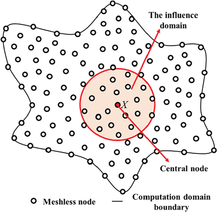
Figure 1: The computation domain of discretization by meshless method

The moment matrix of the polynomial is

PmT=[11⋯1x1x2⋯xny1y2⋯yn⋮pm(x1)⋮pm(x2)⋱⋯⋮pm(xn)] (10)

However, there are n + m variables in Eq. (8), and solving for the coefficient matrices a and b requires adding a little more than m constraints.

∑i=1npj(xi)ai=PmTa=0,j=1,2,⋯,m (11)

Associative Eqs. (8) and (11) lead to the following matrix equation:

U~s=[Us0]=[R0PmPmT0][ab]=Ga0 (12)

Since the matrix R0 is symmetric, the matrix G will also be symmetric, then the coefficient vector a0=G−1U~s , which is carried into Eq. (7) yields

u(x)=NT(x)U~s,NT(x)={RT(x)pT(x)}G−1 (13)

where N(x) is the shape function vector. The radial basis interpolation method obtains the approximate shape function of the unknown function in the influence domain with δ-function property, which is easy to impose the essential boundary conditions.

For equation discretization, this paper utilizes the WLS technique for computational domain solution. The WLS method effectively addresses stability issues associated with meshless discretization formats from the local Petrov-Galerkin method’s computational instability. The local Petrov-Galerkin method generally establishes meshless discretizations based on moving least squares approximation for constructing approximate shape functions, which is computationally expensive without the δ-function property, complicating essential boundary conditions. In contrast, the meshless interpolation approach employing radial basis functions, as adopted here, constructs shape functions with δ-function properties, simplifying essential boundary conditions like controlled bottom-hole flowing pressure. Section 2.3 will present the fundamental principles of the WLS methodology.

2.3 Weighted Least Squares Meshless Methods

Numerous problems ultimately reduce to solving differential equations with defined boundary and initial conditions, meaning the unknown function u(x) must satisfy the differential equation set.

A[u(x)]={A1[u(x)]A2[u(x)]⋮Am1[u(x)]}=0,u∈Ω (14)

Boundary condition

B[u(x)]={B1[u(x)]B2[u(x)]⋮Bm2[u(x)]}=0,u∈∂Ω (15)

where Ai and Bi are differential operators of independent variables.

Since Eq. (14) is satisfied at any point in the domain Ω and Eq. (15) is satisfied at any point on the boundary ∂Ω , it follows that for any functions υ and υ¯ there are

∫ΩυTA[u(x)]dΩ+∫∂Ωυ¯TB[u(x)]d(∂Ω)=0 (16)

The functions υ and υ¯ are termed weight functions, which are function vectors of order m1 and m2 , respectively, and Eq. (16) is the equivalent integral form of the differential equation system (14) and boundary condition Eq. (15). Let uh(x) denote an approximate solution of Eqs. (14) and (15), called the trial function, expressible as a linear combination of a known function set ϕi(x) , namely:

u(x)≈uh(x)=∑i=1nϕi(x)ui=Φ(x)Us (17)

where Us={u1u2u3⋯un}T , ΦT(x)={ϕ1(x)ϕ2(x)⋯ϕn(x)} , ui are parameters to be determined. Obviously, the approximate solutions uh(x) are generally not equal to the exact solutions and they will produce residuals R and R¯ .

R(x)=A[uh(x)],R¯(x)=B[uh(x)] (18)

To obtain the best approximation of the unknown function u(x) , weighting is used to make the residues R and R¯ zero. In weighted least squares, the weighted discrete sum of the residuals R and R¯ squared is made to be

JR=∑k=1r1αkRT(xk)R(xk)+∑k=1r2βkR¯T(xk)R¯(xk) (19)

where αk and βk are the weighting coefficients; xk denotes the coordinates of the matching point; r1 represents the quantity of matching points for calculating the differential equation residuals; r2 signifies the number of matching points for determining the boundary condition residuals. Eq. (19) is attained by minimizing

∂JR∂u=∑k=1r1αk(∂R(xk)∂uj)TR(xk)+∑k=1r2βk(∂R¯T(xk)∂uj)TR¯(xk)=0 (20)

The preceding equation determines the trial function’s n unsolved coefficients. WLS technique necessitates computing residuals at collocation points sans grid background, with the resultant matrix for solving symmetric and less computationally time-intensive vs. the Petrov-Galerkin method, but mandating higher order trial function continuity [28].

3  Meshless Discretization in Low Permeability Tight Reservoirs

The weighted residual methodology is extensively utilized in meshless techniques, constituting an important theoretical foundation for solving intricate control equation discretization. In reservoir engineering, it is often necessary to deal with flow control equations, and traditional finite difference or finite element methods may be limited in handling complex geometric features. To discretize the computational domain and flow control equations more simply and efficiently, this paper utilizes meshless nodal discretization for representing the computational domain. Radial basis point interpolation techniques construct approximate shape functions within the reservoir computational domain. The WLS method discretizes the control equations. This approach demonstrates strong adaptability and efficiency in handling complex geometries and unstructured grids. The established meshless discretization format of the low-permeability tight oil reservoir two-phase flow model is

{∇(λfot∇pft+1)+∇(λfwt∇pft+1)+σkmμo(pmt−pft+1)−(ϕfCtf)tpft+1−pft∂t=0∇(λfwt∇pft+1)−ϕftSwt+1−Swt∂t=0σkmμo(pmt+1−pft+1)+ϕmCtmpmt+1−pmt∂t=0 (21)

Assuming that the reservoir computational domain Ω and boundary Г are discretely characterized by n points. Based on the radial basis point interpolation shape functions approximation, the fracture system pressure, matrix system pressure, and water saturation are expressed as a function of the following approximation:

{pf(x,y)≈∑i=1nNi(x,y)pfi=N(x,y)pfpm(x,y)≈∑i=1nNi(x,y)pmi=N(x,y)pmSw(x,y)≈∑i=1nNi(x,y)Swi=N(x,y)SwN(x,y)=[N1(x,y),N2(x,y),⋯,Nn(x,y)]pf=[pf1,pf2,⋯,pfn]Tpm=[pm1,pm2,⋯,pmn]T (22)

where Ni(x,y) denotes the shape function value of the ith node at the point (x, y), and pfi signifies the fracture pressure at the i-th node, which will be abbreviated as N(x,y) subsequently.

Subsequently, exemplifying with the fracture system seepage control equation, the meshless discretization format for the OW two-phase flow equation will be derived. The residuals are attained by substituting the preceding OW two-phase flow Eq. (22) into Eq. (21).

Rpf(x,y)=[∂N∂x(λfwt+λfgt)∂N∂x+∂N∂y(λfwt+λfgt)∂N∂y+N(λfwt+λfgt)⋅×(∂2N∂x2+∂2N∂y2)]pft+1+σkmμg(Npmt−Npft+1)−(ϕfCtfΔt)t(Npft+1−Npft) (23)

At every computational domain point, the residual Eq. (23) must be satisfied. In other words, boundary points meet the prescribed pressure boundary condition, while internal nodes satisfy Eq. (23). Hence, solving Eq. (23) can be bifurcated into computing the weighted residual for both internal and boundary nodes. As an illustration, the outer constant pressure boundary condition and inner point constant pressure boundary condition are aggregated, therefore the WLS computational format for the fracture system pressure equation is

Πpf=∫Ω(Rpf)TRpfdΩ+∫Γ1α1(Npft+1−pfc)(Npft+1−pfc)dΓ+∫Γ2α2(Npft+1−pi)(Npft+1−pi)dΓ (24)

where α1 and α2 are boundary condition penalty functions. The main idea of the WLS meshless method is to minimize the value of the square of the residual expressed in Eq. (24), when the generalization of Eq. (24) is equal to 0, so that we can get

δΠpf=∑s=1n(δRpf)TRpf|(x,y)=(xs,ys)+∑s=1n1α1NT(Npft+1−pfc)|(x,y)=(xs,ys)+∑s=1n1α2NT(Npft+1−pi)|(x,y)=(xs,ys)=0 (25)

Meshless interpolation methods based on radial basis functions are used to construct shape functions, which possess delta function properties, facilitating the application of essential boundary conditions. The WLS method establishes the variational principle of the unknown problem system equations directly using the least squares method, eliminating residuals at boundary nodes and introducing stabilization terms to form symmetric coefficient matrices. Compared to collocation methods that require background grid integration and Gaussian integration, this approach involves less computational effort [29]. This paper utilizes radial basis functions based on local support domains to construct interpolation functions and employs the WLS method for equation discretization. This synthesis of both methods not only makes the application of essential boundary conditions convenient but also ensures higher computational accuracy and efficiency, making it suitable for characterizing the complex geometries of actual reservoirs.

4  Numerical Examples

As illustrated in Fig. 2, taking well X in a certain block as an example and to account for complex reservoir boundary conditions while simplifying the description, the computational domain is assumed to be an area with an arc boundary. Γ1 , Γ3 represent the left and right boundaries, respectively, forming an arc with a radius of 100 meters. Γ2 , Γ4 are the top and bottom boundaries, respectively, forming straight lines each 300 meters long. All boundaries are set as fixed pressure boundary conditions. Centrally within the computational domain, a horizontal well with six 60-meter half-length radiating fractures exists. Figs. 3 and 4 respectively demonstrate the reservoir models discretized per the Discrete Fracture Model (DFM) and meshless technique. The DFM utilizes 1400 triangular grids, while the meshless model comprises 198 nodes. Significantly, the Discrete Fracture Model (DFM) solution is derived via COMSOL software computations employing fine triangular discretization. Table 1 presents the formation’s physical parameters.

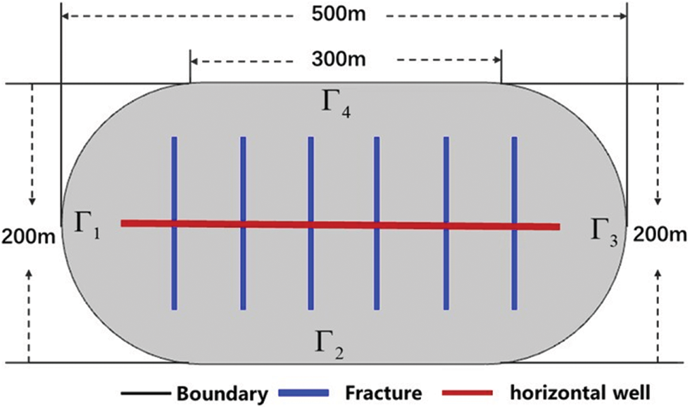
Figure 2: Reservoir model

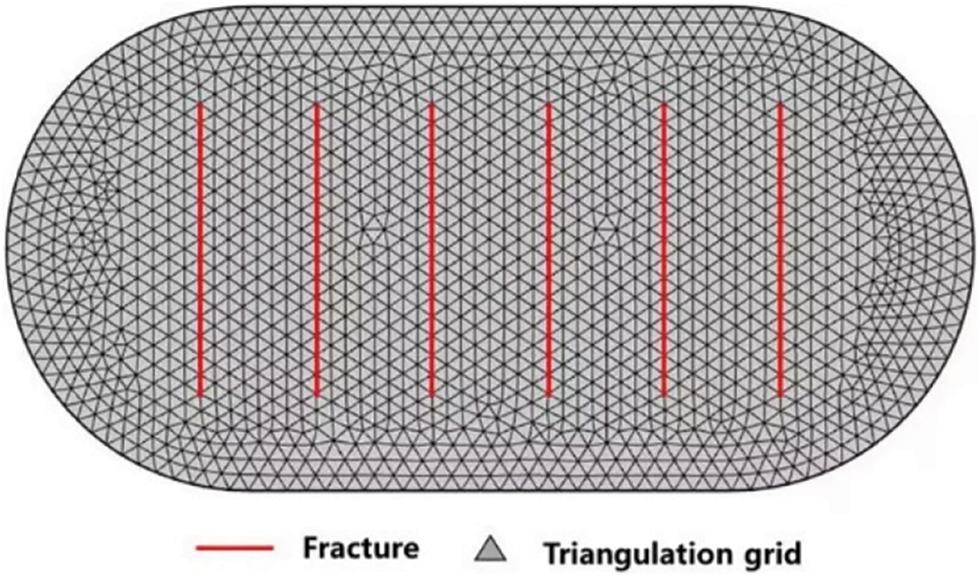
Figure 3: DFM discrete model

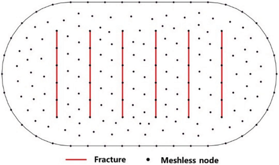
Figure 4: Meshless discrete model

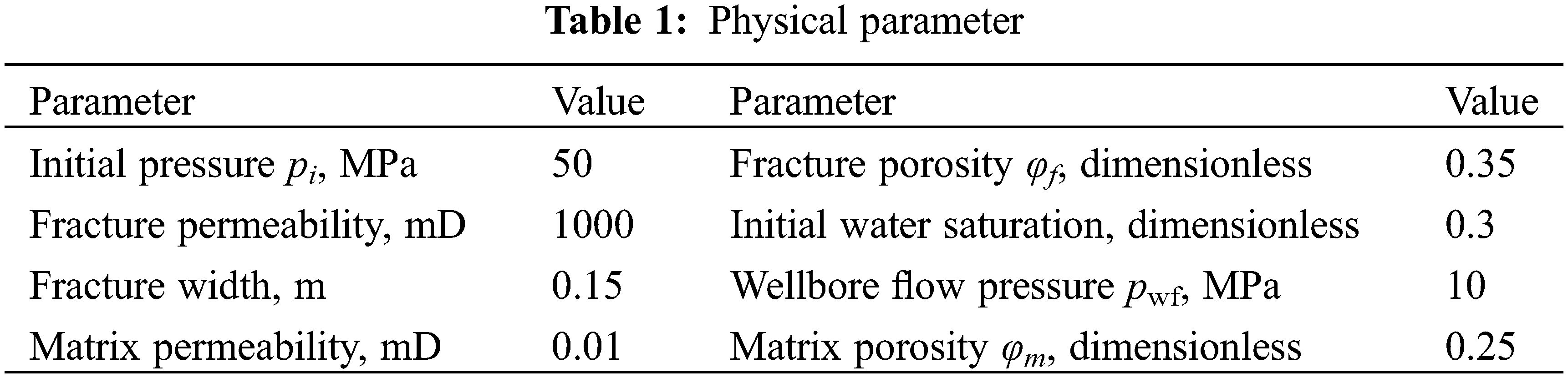
The reservoir model’s initial pressure is established at 50 MPa, and the external boundary is also maintained at 50 MPa. Positioned at the reservoir center along the x-axis is a fractured horizontal well designated for production, with a consistent pressure of 10 MPa. In this investigation of dual-porosity fractured horizontal well models for OW two-phase flow, the fracture pressure at fracturing cluster points is defined as 10 MPa. Table 1 outlines additional fundamental physical properties. The simulation duration spans 150 days, employing a time step of 0.1 day.

Fig. 5 displays the fracture pressures calculated for the first and hundredth days. Even with a relatively coarse model, the meshless method achieved results consistent with those obtained using the finely meshed DFM. Using the DFM results as a reference solution, the pressure calculation accuracy on the 1and 100 days was 97.8% and 98.2%, respectively. In Fig. 6, a comparison is presented between the daily oil and water production curves obtained through the proposed method in this paper and the Discrete Fracture Model (DFM). The results demonstrate a striking similarity, indicating that our method closely aligns with the finely meshed DFM outcomes. The accuracy for daily oil and water production was calculated to be 96.5% and 94.8%, respectively, demonstrating the effectiveness of our method. The notable reduction in computation time observed in our method, in comparison to the finely meshed Discrete Fracture Model (DFM), can be attributed primarily to the meshless method’s ability to provide a more streamlined representation of intricate geometrical features and a lower degree of freedom in the established model. Despite having relatively fewer degrees of freedom, our method successfully produces results that closely match those of the finely meshed DFM. This suggests that the meshless method introduced in this paper is better suited for reservoirs with complex boundaries than the conventional grid-based DFM method.

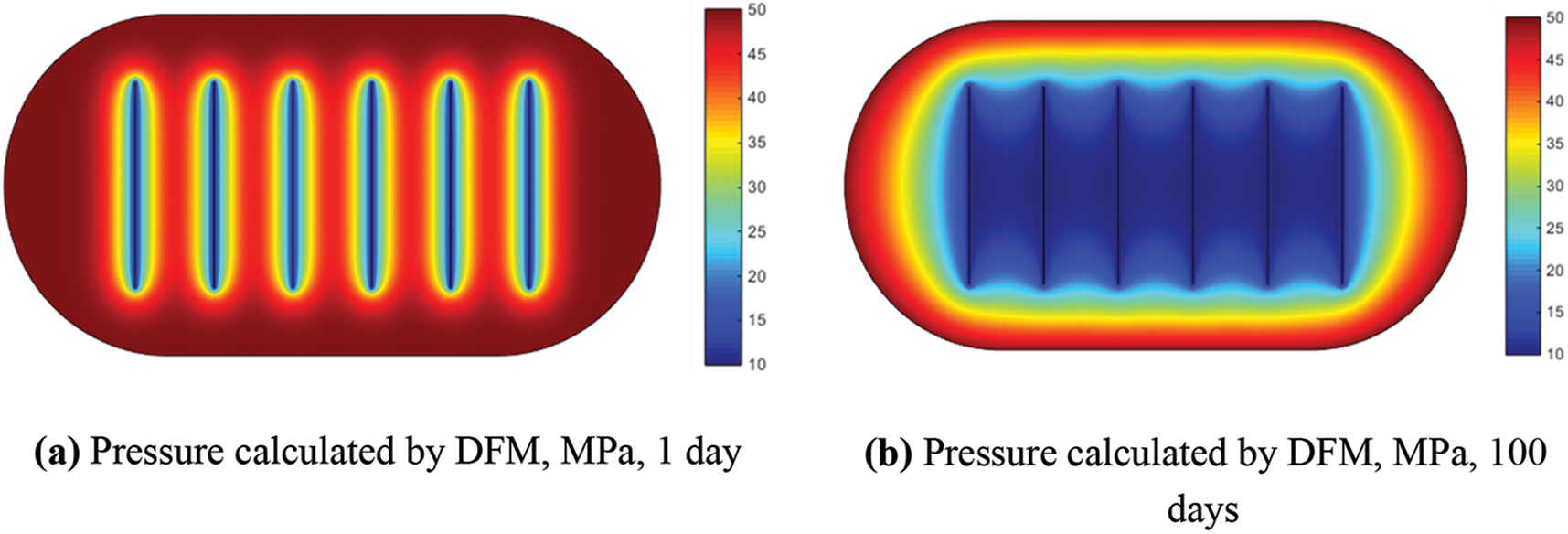
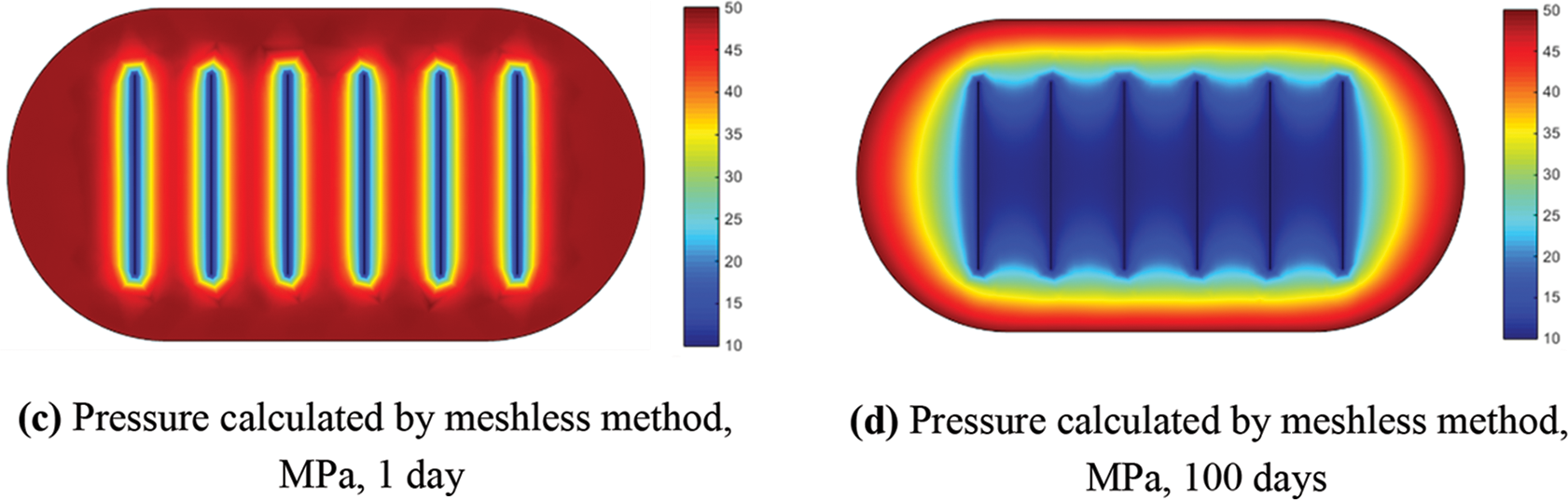
Figure 5: Comparison between the pressure calculated by DFM and the meshless method.

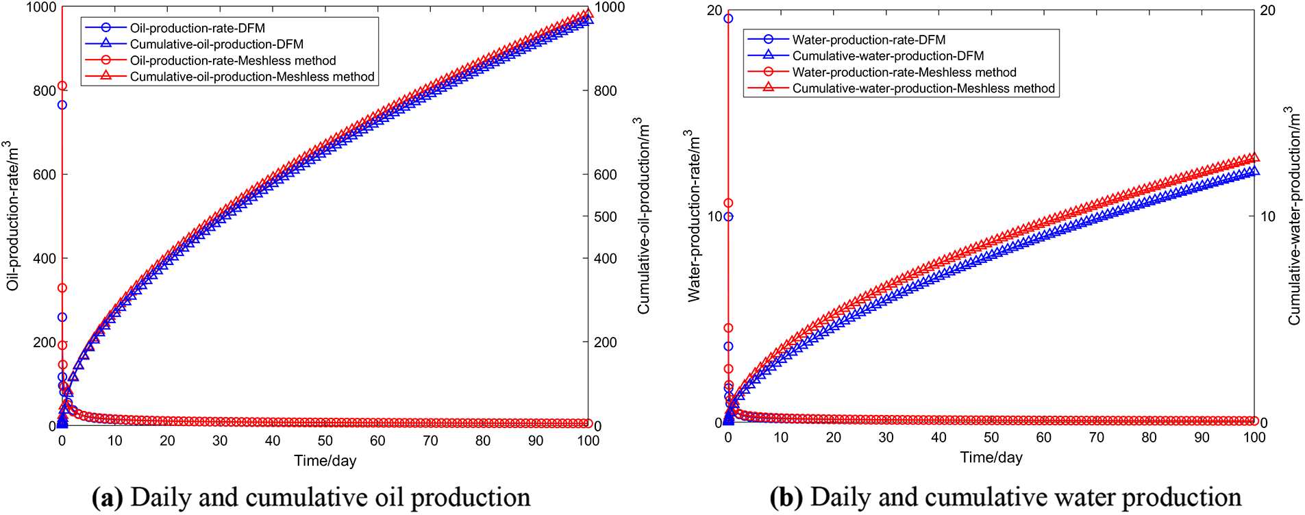
Figure 6: Comparison of oil-production and water-production rate calculated by meshless method and DFM

In-depth analysis focused on the distinct influence of fracture half-length on production. The model, depicted in Fig. 2, incorporates a horizontal well featuring six fractures, each with varying half-lengths of 40, 60, and 80 m. Specifically, Figs. 7 and 8 illustrate the pressure field for fracture half-lengths of 40 and 80 m, respectively. Fig. 9 offers a comprehensive comparison, highlighting the diverse effects of varying fracture half-lengths on production.

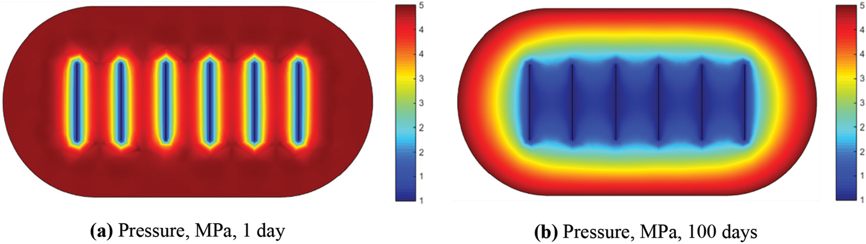
Figure 7: Meshless pressure profile with fracture half-length of 40 m

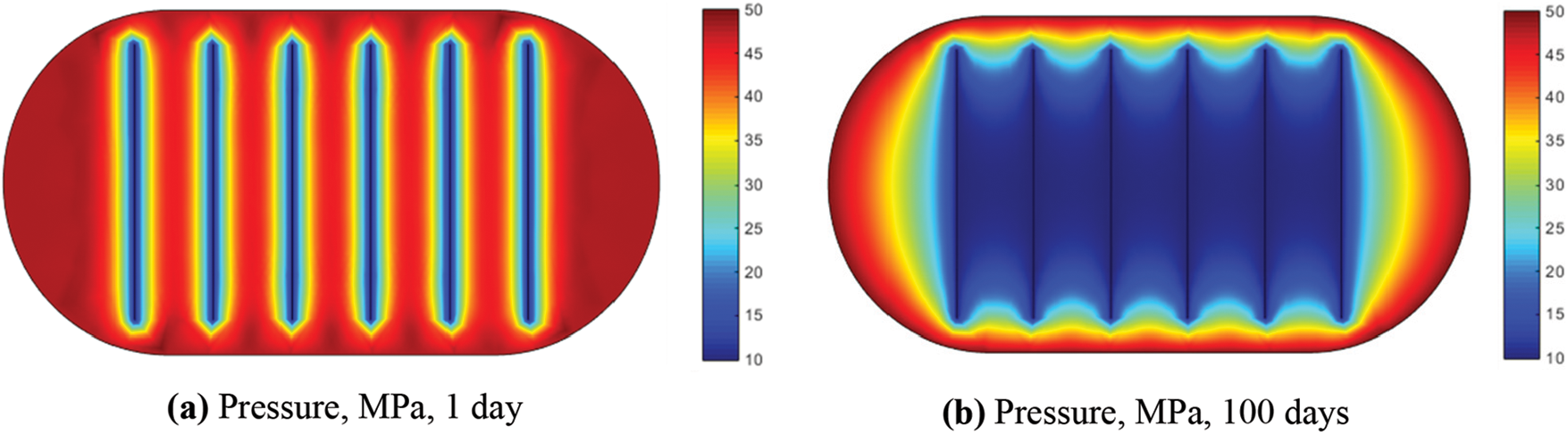
Figure 8: Meshless pressure profile with fracture half-length of 80 m

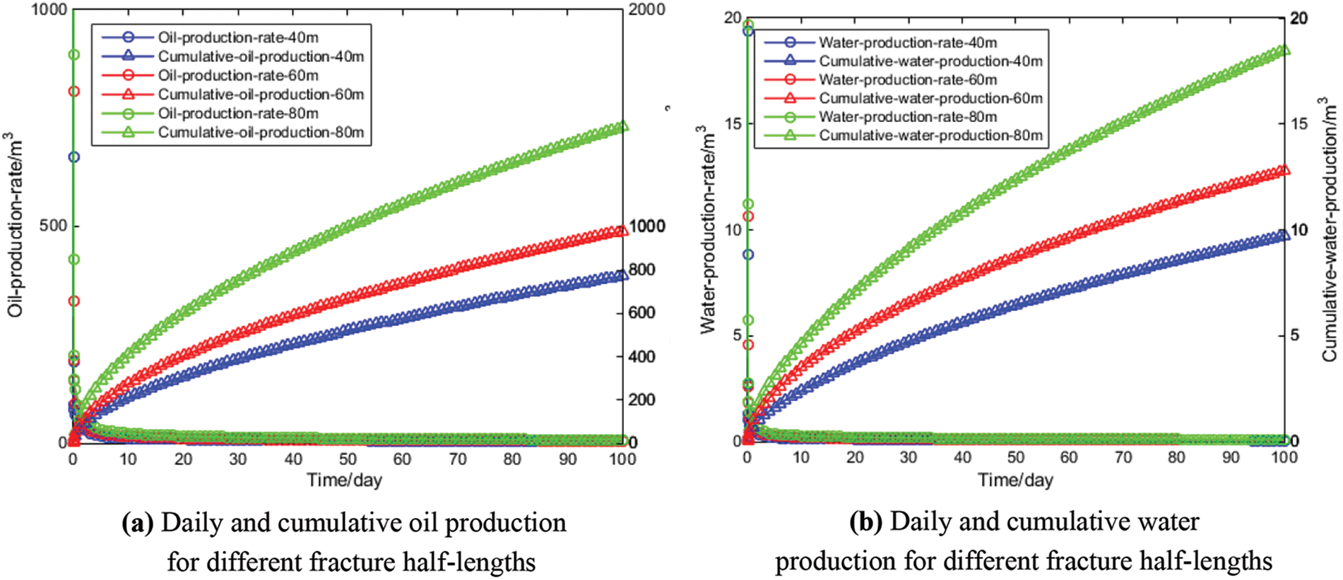
Figure 9: Comparison of oil-production and water-production rate with different fracture half-length

Fig. 9 illustrates the relationship between fracture half-length and both daily and cumulative oil production. It can be observed from the Fig. 9 that as the fracture half-length increases, both daily oil production and cumulative oil production show a positive correlation and increase accordingly. This implies that increasing the half-length of hydraulic fractures can enhance the productivity of fractured wells. This is because when hydraulic fracturing is conducted, increasing the half-length of the fractures enlarges both their length and surface area, thereby enhancing the permeability and fluidity of the rock reservoir. As a result, more crude oil can be released from the rock reservoir, leading to an increase in both daily and cumulative oil production. From the numerical example of this horizontal well, we can observe that the meshless method achieved results consistent with those of the finely meshed Discrete Fracture Model (DFM), which validates the correctness of the method presented in this paper. The meshless method, based on a point cloud, discretizes the reservoir’s computational domain more freely and flexibly, making it simpler to finely delineate the complex geometry of the reservoir. With a smaller degree of freedom in the model, we obtained higher computational accuracy, indicating that our method can achieve high precision in calculations without generating a high-resolution matching point cloud when discretizing complex boundaries. Of course, theoretically, a high-resolution point cloud can achieve more accurate results but at the cost of increased computational time. Therefore, compared to high-resolution grid-based methods, the meshless method can achieve a better balance between computational efficiency and accuracy.

5  Conclusions

1. This study combines the OW two-phase flow model and dual-porosity theory for low-permeability tight reservoirs. It integrates the WLS meshless method, employing radial basis point interpolation functions to formulate shape functions. Consequently, a meshless computational model is established for horizontal well productivity in low-permeability tight reservoirs with circular curved boundaries. The model successfully predicts production dynamics, specifically addressing fractured horizontal wells with varying fracture half-lengths.

2. The meshless method presented in this paper achieves commendable results, surpassing 98.2% accuracy in pressure calculations, even with a reduced number of degrees of freedom compared to the finely meshed Discrete Fracture Model (DFM) used as a reference solution. Notably, our method is versatile, demonstrating adaptability in describing reservoirs featuring complex boundaries or geological conditions, effectively handling intricate geometries.

3. An analysis of the impact of fracture half-length on both daily and cumulative oil production of fractured horizontal wells was conducted. The findings reveal a positive correlation between fracture half-length and both daily and cumulative oil production. To maximize cumulative oil production, it is suggested to enhance fractured well productivity by increasing the half-length of hydraulic fractures.

Acknowledgement: None.

Funding Statement: The authors received no specific funding for this study.

Author Contributions: The authors confirm contribution to the paper as follows: study conception and design: XL; data collection: XL; analysis and interpretation of results: XL, KY, BF; draft manuscript preparation: KY, XS, DF, LY. All authors reviewed the results and approved the final version of the manuscript.

Availability of Data and Materials: The data that support the findings of this study are available from the corresponding author, upon reasonable request.

Conflicts of Interest: The authors declare that they have no conflicts of interest to report regarding the present study.

References

1. Zhang Z, Zhu G, Han J, Jiang S, Li J, Chi L. Tectono-thermal impacts on the formation of a heavy oil in the eastern Tarim Basin (Chinaimplications for oil and gas potential. J Petrol Sci Eng. 2022;208:109353. [Google Scholar]

2. Warpinski NR. Hydraulic fracturing in tight, fissured media. J Petrol Technol. 1991;43(2):146–209. [Google Scholar]

3. Zhang X, He C, Zhou J, Tian Y, He L, Sui H, et al. Demulsification of water-in-heavy oil emulsions by oxygen-enriched non-ionic demulsifier: synthesis, characterization and mechanisms. Fuel. 2023;338:127274. [Google Scholar]

4. Zheng Y, Zhai C, Sun Y, Cong Y, Tang W, Yu X, et al. Effect of reservoir temperatures on the stabilization and flowback of CO2 foam fracturing fluid containing nano-SiO2 particles: an experimental study. Geoenergy Sci Eng. 2023;212048. [Google Scholar]

5. Suri Y, Islam SZ, Hossain M. Numerical modelling of proppant transport in hydraulic fractures. Fluid Dyn Mater Process. 2020;16(2):297–337. doi:https://doi.org/10.32604/fdmp.2020.08421. [Google Scholar] [CrossRef]

6. Isah A, Hiba M, Al-Azani K, Aljawad MS, Mahmoud M. A comprehensive review of proppant transport in fractured reservoirs: experimental, numerical, and field aspects. J Nat Gas Sci Eng. 2021;88:103832. [Google Scholar]

7. Snow DT. Rock fracture spacings, openings, and porosities. J Soil Mech Found Div. 1968;94(1):73–91. [Google Scholar]

8. Warren JE, Root PJ. The behavior of naturally fractured reservoirs. SPE J. 1963;3(3):245–55. [Google Scholar]

9. Pruess K, Narasimhan TN. A practical method for modeling fluid and heat flow in fractured porous media. SPE J. 1985;25(1):14–26. [Google Scholar]

10. Slough KJ, Sudicky EA, Forsyth PA. Grid refinement for modeling multiphase flow in discretely fractured porous media. Adv Water Resour. 1999;23(3):261–9. [Google Scholar]

11. Yaghoubi A. Hydraulic fracturing modeling using a discrete fracture network in the Barnett Shale. Int J Rock Mech Min Sci. 2019;119:98–108. [Google Scholar]

12. Karimi-Fard M, Firoozabadi A. Numerical simulation of water injection in fractured media using the discrete fractured model and the Galerkin method. SPEREE. 2003;6(2):117–126. [Google Scholar]

13. Monteagudo JEP, Firoozabadi A. Control-volume method for numerical simulation of two-phase immiscible flow in two-and three-dimensional discrete-fractured media. Water Resour Res. 2004;40(7). doi:https://doi.org/10.1029/2003WR002996. [Google Scholar] [CrossRef]

14. Rao X, Zhao H, Liu Y. A meshless numerical modeling method for fractured reservoirs based on extended finite volume method. SPE J. 2022;27(6):3525–64. [Google Scholar]

15. Zhan WT, Zhao H, Rao X, Liu W, Xu YF. Numerical simulation of multi-scale fractured reservoir based on connection element method. Chin J Theor Appl Mech. 2023;55(7):1570–81 (In Chinese). [Google Scholar]

16. Bernard PS. A deterministic vortex sheet method for boundary layer flow. J Comput Phys. 1995;117(1):132–45. [Google Scholar]

17. Rao X, Liu Y, Zhao H. An upwind generalized finite difference method for meshless solution of two-phase porous flow equations. Eng Anal Bound Elem. 2022;137:105–18. [Google Scholar]

18. Zhan W, Rao X, Zhao H, Zhang H, Hu S, Dai W. Generalized finite difference method (GFDM) based analysis for subsurface flow problems in anisotropic formation. Eng Anal Bound Elem. 2022;140:48–58. [Google Scholar]

19. Monaghan JJ. Smoothed particle hydrodynamics and its diverse applications. Annu Rev Fluid Mech. 2012;44:323–46. [Google Scholar]

20. Atluri SN, Sladek J, Sladek V, Zhu T. The local boundary integral equation (LBIE) and its meshless implementation for linear elasticity. Comput Mech. 2000;25(2–3):180–98. [Google Scholar]

21. Atluri SN, Zhu TL. The meshless local Petrov-Galerkin (MLPG) approach for solving problems in elasto-statics. Comput Mech. 2000;25(2–3):169–79. [Google Scholar]

22. Zhang X, Hu W, Pan XF, Lu MW. Meshless weighted least-square method. Acta Mech Sin (Chin Ed). 2003;35(4):425–31. [Google Scholar]

23. Honarbakhsh B, Tavakoli A. Numerical solution of the EFIE by the meshfree collocation method. Eng Anal Bound Elem. 2013;37(1):153–61. [Google Scholar]

24. Kiran R, Nguyen-Thanh N, Huang J, Zhou K. Buckling analysis of cracked orthotropic 3D plates and shells via an isogeometric-reproducing kernel particle method. Theor Appl Fract Mech. 2021;114:102993. [Google Scholar]

25. Huang J, Nguyen-Thanh N, Gao J, Fan Z, Zhou K. Static, free vibration, and buckling analyses of laminated composite plates via an isogeometric meshfree collocation approach. Compos Struct. 2022;285:115011. [Google Scholar]

26. Xu Y, Sheng G, Zhao H, Hui Y, Zhou Y, Ma J, et al. A new approach for gas-water flow simulation in multi-fractured horizontal wells of shale gas reservoirs. J Petrol Sci Eng. 2021;199:108292. [Google Scholar]

27. Rao X, Zhan W, Zhao H, Xu Y, Liu D, et al. Application of the least-square meshless method to gas-water flow simulation of complex-shape shale gas reservoirs. Eng Anal Bound Elem. 2021;129:39–54. [Google Scholar]

28. Park SH, Youn SK. The least-squares meshfree method. Int J Numer Methods Eng. 2001;52(9):997–1012. [Google Scholar]

29. Min Z, Wen C. A meshless weighted least square method based on radial basic functions. Chin J Comput Mech. 2011;28(1):66–71 (In Chinese). [Google Scholar]