
 Submit a Paper
 Propose a Special lssue
 Open Access
ARTICLE
Study on the Relationship between Structural Aspects and Aerodynamic Characteristics of Archimedes Spiral Wind Turbines
1 Mechanical and Electrical Engineering Institue, Xinjiang Agricultural University, Urumqi, 830052, China
2 College of Mechanics, Shanghai DianJi University, Shanghai, 201306, China
3 School of Energy Engineering, Xinjiang Institute of Engineering, Urumqi, 830023, China
* Corresponding Author: Yuanjun Dai. Email:
Fluid Dynamics & Materials Processing 2024, 20(7), 1517-1537. https://doi.org/10.32604/fdmp.2024.046828
Received 16 October 2023; Accepted 07 February 2024; Issue published 23 July 2024
 View Full Text
 Download PDF
Abstract
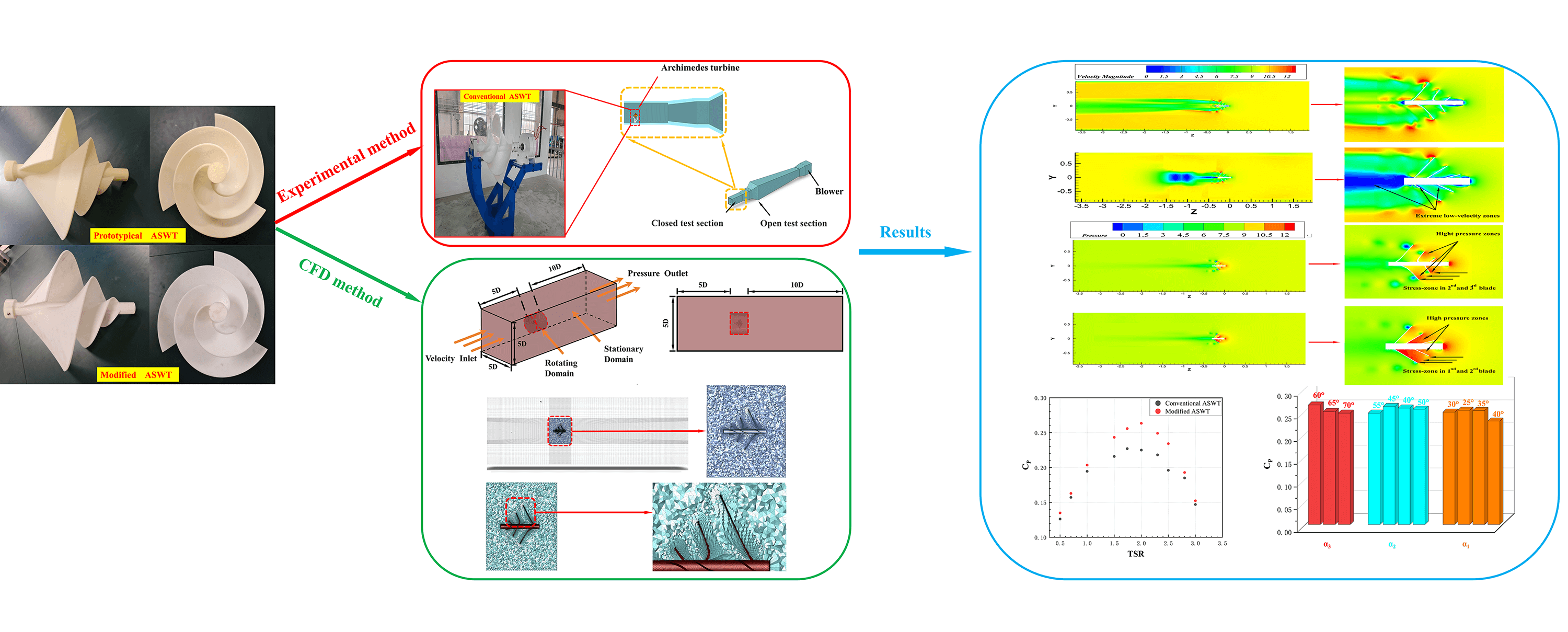
A combined experimental and numerical research study is conducted to investigate the complex relationship between the structure and the aerodynamic performances of an Archimedes spiral wind turbine (ASWT). Two ASWTs are considered, a prototypical version and an improved version. It is shown that the latter achieves the best aerodynamic performance when the spread angles at the three sets of blades are α = 30°, α = 55°, α = 60°, respectively and the blade thickness is 4 mm. For a velocity V = 10 m/s, a tip speed ratio (TSR) = 1.58 and 2, the maximum C values are 0.223 and 0.263 for the prototypical ASWT and improved ASWT, respectively, and the maximum C enhancement is 17.93%. For V = 10 m/s and TSR = 2, the C values of the prototypical ASWT and improved ASWT are 0.225 and 0.263, respectively, with an aerodynamic performance enhancement of 16.88%. Through mutual verification of the test outcomes and numerical results, it is concluded that the proposed approach can effectively lead to aerodynamic performance improvement.Graphic Abstract
Keywords
Nomenclature
| S | Turbine sweeping area (m2) |
| CT | Turbine torque coefficient |
| CP | Turbine power coefficient |
| D | Turbine diameter (m) |
| n | Turbine rotational speed (r/s) |
| T | Turbine output torque (N.m) |
| V | Incoming flow wind speed |
| k | Turbulent kinetic energy (m2/s2) |
| R | Turbine radius (m) |
| Ma | Mach number |
| y+ | Non-dimensional wall distance |
| Re | Reynolds number |
| M | Measured parameter |
| u | Error |
| FD | Obstructive force (N) |
| FDx | Obstructive force parallel to x direction (N) |
| FDy | Obstructive force perpendicular to y direction (N) |
| FL | Lift force (N) |
| FLx | Lift force parallel to x direction (N) |
| FLy | Lift force perpendicular to y direction (N) |
| α | Unfolded angle at the blade (°) |
| ν | Kinematic viscosity (m2/s) |
| μ | Dynamic viscosity of the air (kg/m.s) |
| μt | The turbulent viscosity (kg/m.s) |
| ώ | Turbine angular speed (rad/s) |
| ρ | Air density (kg/m3) |
| ω | Turbulent dissipation rate |
| ASWT | Archimedes Spiral Wind Turbine |
| HAWT | Horizontal-axis wind turbine |
| VAWT | Vertical-axis wind turbine |
| RANS | Reynolds-Averaged Navier-stokes |
| MRF | Multiple Reference Frame |
| CFD | Computational fluid dynamics |
| RE | Relative error |
| TSR | Tip-speed ratio |
| FVM | Finite volume method |
From 2023 onwards, countries worldwide are emphasizing the reliability of energy supply. The emergence of solar panels, while costly to manufacture, prone to damage, and environmentally polluting, has prompted the search for ways to enhance the efficient use of energy, becoming a new consensus. Renewable energy systems [1] have been proposed to offer economically viable options for countries in developing regions that lack infrastructure like power grids [2–4]. Wind energy, among these systems, stands out as a renewable and clean energy source with vast reserves and wide distribution, despite its low energy density and inherent instability. Given specific technical conditions, wind energy can be harnessed as a significant energy source. The technology for converting energy resources [5–7] through wind turbines has rapidly advanced, although its implementation faces challenges, particularly in urban areas, due to technological limitations and space constraints.
Wind turbines typically follow the format of Horizontal Axis Wind Turbines (HAWT) and Vertical Axis Wind Turbines (VAWT) [8–11]. Zhang et al. [12] utilized numerical simulation to study the changes in airfoil structure to evaluate the aerodynamic performance of VAWT under the optimal tip speed ratio. The results indicated that the optimized winglet structure could reduce the tip vortex size, thus improving aerodynamic efficiency. In another study, Zhang et al. [13] employed a CFD-based method to investigate how the maximum curvature of a three-dimensional airfoil structure along the chord direction affects the aerodynamic performance of a vertical-axis wind turbine. Building on these research ideas, the main focus of this paper is the Archimedes Spiral Wind Turbine (ASWT). ASWT is a novel wind turbine design concept based on the modeling idea of the Archimedes spiral equation. The designed spiral structure enables free airflow inside the blades. The three-bladed structure, combined with a 120° circumferential array distribution, incorporates features of both HAWT and VAWT, leveraging their drag and lift characteristics [14,15]. It has the speed regulation characteristics under the wider tip speed ratio (TSR) conditions, and the power coefficient value measured under the optimal tip speed ratio is the best. Hossam et al. [14] in this work by designing a shroud with a flange at its inlet during an optimization technique aims to maximize the coefficient of power (Cp). the results show that at TSR = 2.5, the Cp value of the optimal enveloped ASWT is up to 0.502, which is 2.58 times that of the bare ASWT (Cp = 0.195).
Currently, research on Archimedes Spiral Wind Turbines includes various studies. Chaudhary et al. [16] designed a yawing system that enables the ASWT to automatically face the direction of incoming wind during operation, achieving the optimal yaw angle for wind energy capture. They demonstrated that the Archimedes spiral wind turbine has the advantage of starting at a minimum incoming wind speed of 2.5 m/s. A comprehensive evaluation of its structural characteristics, with good passive yawing effects and low wind input, along with high torque characteristics, makes it applicable in urban areas. Rao et al. [17] studied its aerodynamic characteristics, conducting both numerical simulation and experimental studies on the Archimedes Wind Turbine (AWT) and Archimedes Airfoil Wind Turbine (AAWT). Song et al. [18] conducted numerical simulations on the ASWT at five different blade spread angles to predict its aerodynamic performance and wake characteristics. Kamal Ahmed et al. [19] compared the numerical simulation and test results of the S-series and NACA-series airfoils, finding a 26.88% improvement in aerodynamic performance over the prototypical ASWT. At present, the latest theoretical research analysis related to this wind turbine is about Kazem et al. [20] based on Archimedes screw turbines (AST), an effective physical model was established and the gray wolf algorithm was verified and compared. The results showed that the optimal values of inner diameter and outer diameter, pitch and ratio to outer diameter, inclination angle, and number of blades were 0.43~0.56, 1~1.2, 20~22.5, and 2~4, respectively, and the optimal optimization parameters were found. To prolong the service life of deep-water exploration equipment, it is necessary to develop a new hydrodynamic turbine with good self-starting capability to utilize low-speed current energy in a deep-water environment. Zhang et al. [21] proposed a new type of pipeless Archimedes screw turbine to improve the start-up performance of the system in low-speed current applications. The results showed that the maximum power coefficient and static torque coefficient of the optimized pipeless Archimedes screw turbine were increased by 36.7% and 143%, respectively compared with the initial design.
However, these studies are limited to the comparison of the angle changes of several sets of single models and do not fully consider the changes in the angle of system division and the analysis of the regular changes of related parameters. In the process of modification, according to the change law of ASWT performance parameters, the movement of the pressure surface area is caused by the modification of ASWT. Therefore, in addition to the strict division of the inclination angle specified on the helix equation in the physical modeling process, the researchers should also ensure a fixed distance between the pitches to explore the influence of the blade spread angle on the aerodynamic performance of ASWT. This paper proposes a geometric-physical model for measuring ASWT. Firstly, the design method of the ASWT model is introduced. Unlike traditional methods, this approach combines voltage and current test results to characterize changes in power. Subsequently, numerical simulations of ASWT with different structures were considered, and the simulation results were compared with the experimental results. Finally, the experimental and numerical methods used in this paper are summarized and prospected.
The distribution of the structure in this paper is mainly as follows: the Section 2 describes the design and manufacturing methods of the blade structure. The Section 3 introduces the planning of test methods and equipment. Section 4 mainly discusses the prototypical ASWT and the improved ASWT with the comparison of simulation cases and test results to characterize their aerodynamic properties. Finally, Section 6 draws conclusions.
2 Blade Design and Manufacturing
In this study, the aerodynamic performance of a prototypical Archimedes Spiral Wind Turbine (ASWT) with a fixed spread angle and an ASWT with a variable blade spread angle is compared and analyzed. The ASWT with the spread angle corresponding to the best aerodynamic performance is determined. Based on achieving the optimal aerodynamic performance working condition, the noise characteristics of the ASWT before and after modification are experimentally calculated.
A prototypical ASWT was designed using UG NX12.0 software to serve as an effective reference for modeling the aerodynamic performance evaluation and numerical simulation of the ASWT. Firstly, the parameters for blade spreading angle and blade helix angle are determined, with the blade diameter of the prototypical ASWT set at 360 mm, and the helix angle ranging from 0° to 360°. The blade spread angle is independent of the helix angle. As depicted in Fig. 1a, the blade helix angle is determined by establishing three equidistant points in the range of 0° to 360° according to Archimedes’ helix equation. The blade spread angle, expressed as α1, α2, α3, represents the angle between the blade and the rotating axis, as illustrated in Fig. 1b. For the design of the single-blade structure, α3 is positioned at a helix angle of 0°, α2 at 120°, and α1 at 240° in the angular displacement plane. Finally, the study of the ASWT is crucial by utilizing the spread angle parameters of three different sets of blades Nawar et al. [22] designed three Prototypical ASWT models with a fixed spread angle of 60° and three improved ASWT models with variable the spread angles of α1 = 30°, α2 = 45°, α3 = 60°. Next, we will subdivide the group angles and perform a grouped blade design. As shown in Table 1, the blade design parameters of the prototypical ASWT involved in this paper include a blade thickness (t) of 4 mm, length-to-diameter ratio (L/D) of 0.90, wind turbine diameter (D) of 360 mm, the number of blades (B) of 3, the spread angle α1 = α2 = α3 = 60° for the three groups of blades, fixed pitch (s) of 126 mm, and the diameter of the rotating shaft (d) of 35 mm, as shown in Figs. 1a and 1b. The blade design parameters of the improved ASWT include a blade thickness (t) of 4 mm, a length-to-diameter ratio (L/D) of 0.90, wind turbine diameter (D) of 360 mm, number of blades (B) of 3, the spread angles α1 = 30°, α2 = 55°, α3 = 60° at three sets of blades, fixed pitch (s) of 96 mm, and rotating axis (d) of 35 mm, as shown in Fig. 2a. The light-cured 3D printing setup parameters include a layer thickness of 0.05 mm, an exposure time of 6 s bottom exposure time of 50 s, anti-aliasing level of 8, support infill density of 20%, and an overall blade model infill density of 100%. The solid models before and after the improvement required for the experiment were light-cured 3D printed using Stereo Lithography Appearance (SLA) [23].
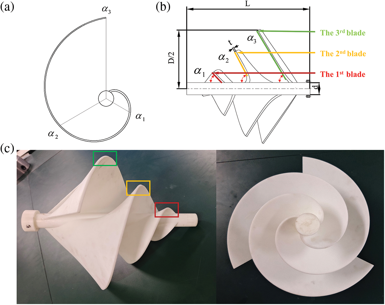
Figure 1: Prototypical ASWT geometry model parameters and printed model
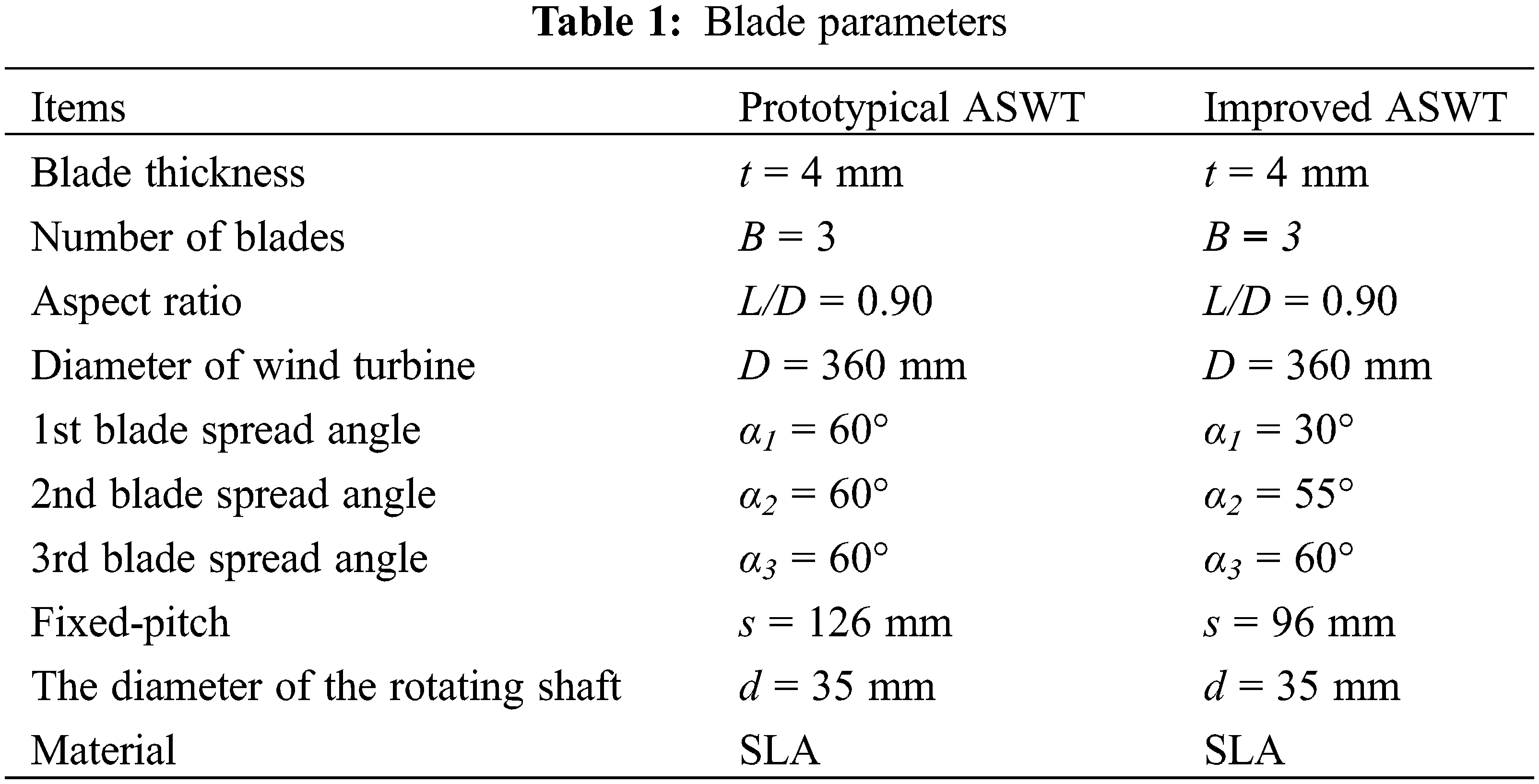
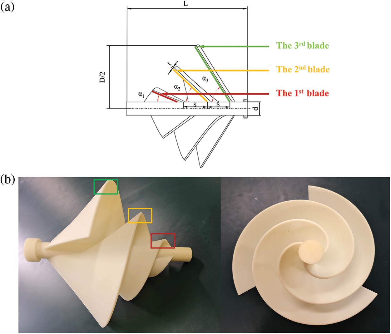
Figure 2: Parameters of improved ASWT geometric model and printed model
The test was conducted in the Key Laboratory of Efficient Energy Utilization of Xinjiang Institute of Engineering (Urumqi, Xinjiang, China). The testing was performed in a low-speed wind tunnel, specifically, the DZS-1400 × 1400/2000 × 2000-I low-speed wind tunnel, which is comprised of an open section (the first test section) and a closed section (the second test section). As the external dimensions of the wind turbine were designed to be that of an Archimedes spiral wind turbine, the aerodynamic performance test was carried out in the closed section of the second test section, as illustrated in Figs. 3 and 4.
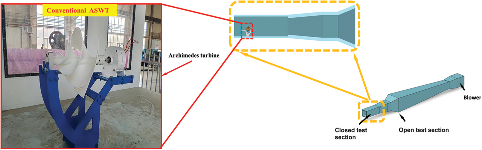
Figure 3: Schematic diagram of the wind tunnel and related installation test locations
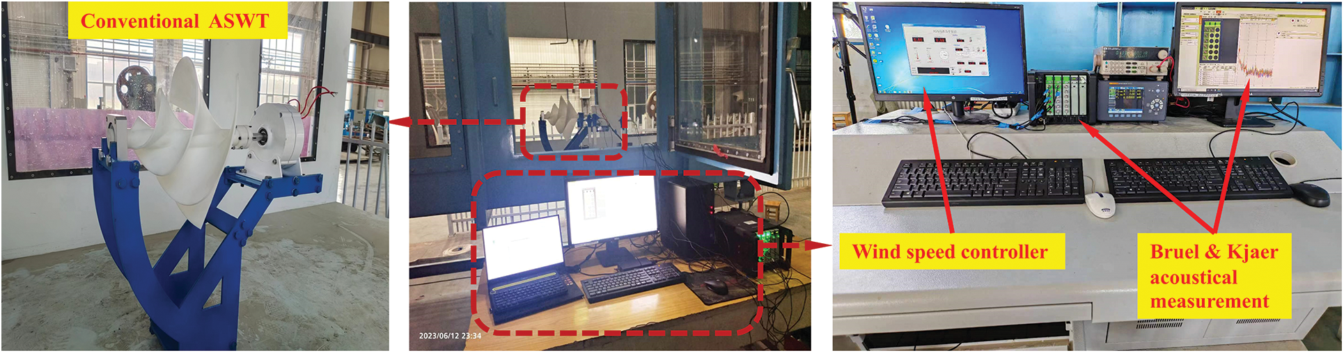
Figure 4: Wind turbines installation and testing platform in closed wind tunnel test section
3.1 Aerodynamic Characteristics and Measuring Equipment
3.1.1 Aerodynamic Characteristics
The aerodynamic characteristics of an ASWT are usually described by a set of dimensionless aerodynamic performance curves [24].
The ASWT test torque is calculated from Eq. (1):
where T is the generated torque, P is the output power, and ω is the angular velocity of the wind turbine.
The power coefficient Eq. (2), the torque coefficient Eq. (3), the force coefficient Eq. (4), and the tip speed ratio Eq. (5) can be calculated from the following equations:
where V is the incoming wind speed, and S is the swept area of the wind turbine when it is facing the incoming wind. ρ is the air density (ρ = 1.225 × 10⁻⁵ kg/m3).
3.1.2 Aerodynamic Measuring Equipment
The measurement equipment includes a power analyzer, as shown in Fig. 5, of type NORMA 4000CN. It has a maximum input voltage of CATII 1000 V and a maximum input current of CATII 1000 A, with an accuracy of ±0.2%. The power values obtained are accurate to two decimal places, which can be used to satisfy the test process by completely measuring the rotational speed and the output power of the ASWT under different working conditions. Aerodynamic performance tests are conducted at a distance from the ASWT. The experiments were conducted in the closed section, specifically 10D from the left side of the open section. The power analyzer and load meter were used in series, and the electronic load meter is shown in Fig. 5, of type IT8512A+.
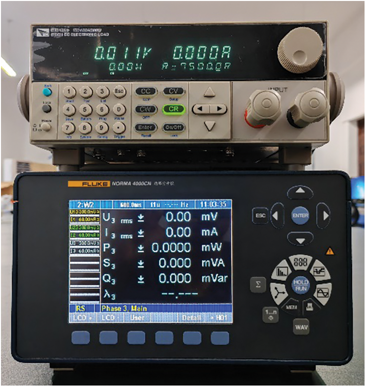
Figure 5: Aerodynamic characteristics and noise measurement process with related equipment: power analyzer type NORMA 4000CN and electronic load meter type IT8512A+
4 Numerical Calculations and Analysis
The geometrical model structure of the ASWT was parametrically designed in UG NX12.0 by establishing the Archimedean helix equation. The designed model was imported into Spaceclaim software for area delineation pre-processing, and then imported into ICEM CFD 2020 R2 and ANSYS-Fluent 2020 R2 Meshing software for structural meshing in the stationary domain and non-structural meshing in the rotating domain, respectively. Finally, the meshes of the two regions were overlapped and imported into the ANSYS-Fluent 2020 R2 solver for the steady-state solution.
4.1 Calculation of the Area Division
The ANSYS-Fluent 2020 R2 software provides a feasible approach to establishing a reasonable meshing and calculation for this computational domain. To obtain accurate calculation results, the meshes in the stationary and rotating domains are refined, respectively. The ANSYS-Fluent 2020 R2 solver, which employs the Navier-Stokes equations (RANS) and the Finite Volume Method (FVM), is capable of meeting the requirements for the accurate prediction of flow fields in the stationary and rotating domains. The rotation domain mesh is refined to ensure the accuracy of predicting the flow field. Additionally, Fig. 6 shows boundary condition settings, such as velocity inlets and pressure outlets.
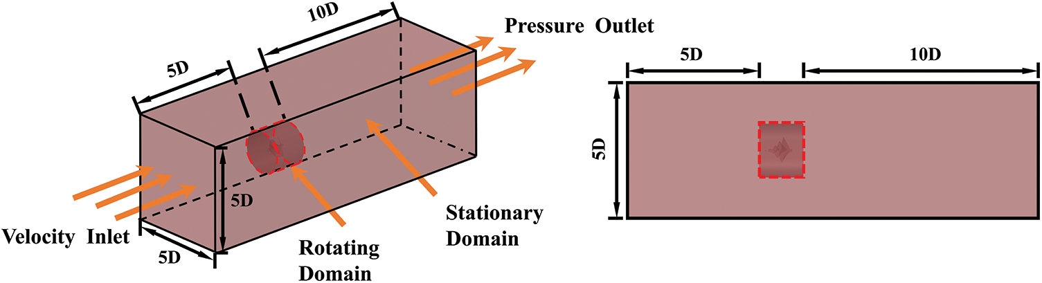
Figure 6: Physical model area division
In Fig. 6, the stationary domain section features a rectangular cross-section (5D), where “D” represents five times the turbine diameter, serving as the velocity inlet. With the downwind direction as the reference, the stationary domain area is delineated both in front of and behind the rotating area, denoted as (5D) and (10D), respectively. The rotating domain dimensions are divided by a cylindrical region with a height of (1.6D) and diameter of (2D). This division is to ensure that the mesh around the blades maintains a skewness less than 0.7 and to guarantee that the final generated body mesh has a minimum orthogonal mass greater than 0.2. The wind speeds flowing through the stationary domain are 4, 6, 8, and 10 m/s, respectively. To obtain accurate calculated values, the above channel data were constructed based on the reference values recommended by Zhang et al. [12]. The actual wind tunnel closed section model.
The meshing of the complete computational region is illustrated in Fig. 7a. Notably, the inflation layer cells around the blade peripheral surface and near the rotating axis surface, as well as the Prism cells, are highlighted in Fig. 7b. The model cell mesh region conditions are based on the method of the rotating coordinate system (MRF). The delineated mesh regions in ANSYS-Fluent include the stationary domain and encrypted region, the rotating domain and mesh interface, the blade surface mesh, and the expansion layer mesh.
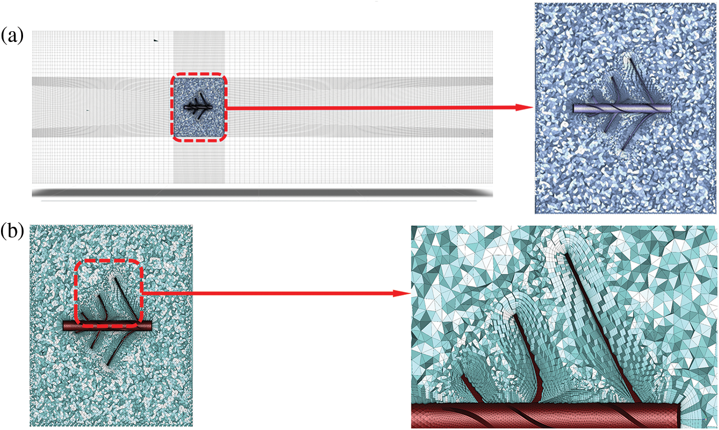
Figure 7: (a) Complete computational domain mesh, (b) Prism layer mesh
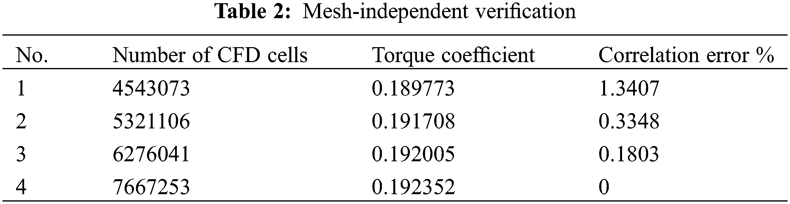
In this case, the growth rate of all the blades and the rotating axis boundary is 1.2. The height of the first layer is 2 × 10⁻⁵ m. The direction of the incoming flow is distributed in the normal direction, so the number of layers of the prismatic layer around the blades is set to 18 to ensure computational convergence, all of which remain unchanged in the mesh independence verification, as shown in Table 2. To ensure that the changes in the size of the cell do not affect the accuracy of the results of the calculations. The gradual incremental increase in the number of grids obtained is 4543073, 7667253, 5321106, and 6276041 cells. All the models above keep y+ < 1 for calculation. The relative error is a minimum of 0.1803%, as shown in Table 2. The prototypical ASWT has a total of 6276041 grid cells, of which the static domain grid cells are about 2701284. The rotational domain grid cells are about 3574757, and the relative error of the grid is 0.1803%, indicating sufficient computational accuracy.
4.2 CFD Turbulence Model Setup
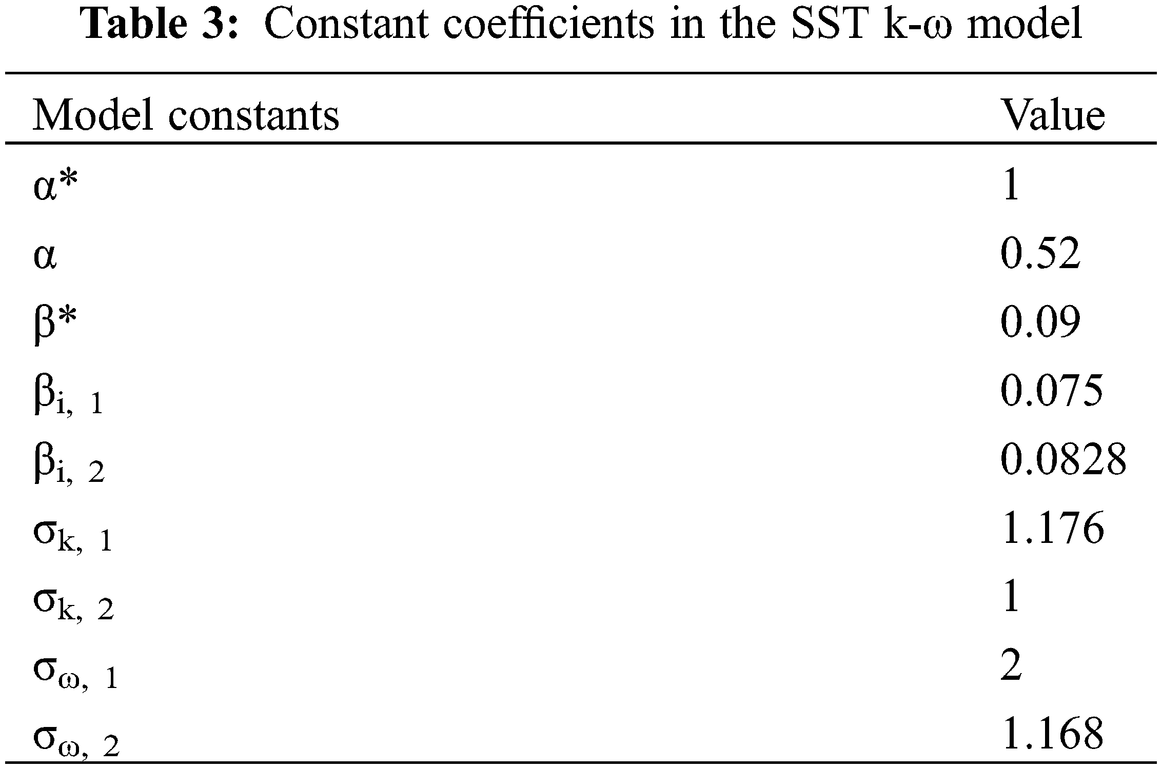
To be able to accurately predict the aerodynamic performance of a prototypical ASWT, the model solution is initially simulated using the RANS equations for the flow field. The numerical solution of the moments is obtained after the convergence of the flow field [25]. Since the flow velocity of the ASWT wind turbine studied in this paper is lower than the Mach number (Ma) of 0.3, it can be simulated as a steady-state incompressible flow by considering the effect of viscous forces on it. The constant coefficients in the SST k-ω model are shown in Table 3.
Momentum Eq. (7):
Reynolds stress tensor Eq. (8):
where
k-ω is SST based on the derivation of the Eqs. (11), (12) shown below [27]:
Gk and Gω are represent the turbulent kinetic energy generated by the mean velocity gradient down k and ω, respectively. Yk and Yω are represent the turbulent dissipation generated by k and ω. Sk and Sω mean it is a user-defined source term, Гk and Гω are represent the effective diffusivity defining k and ω, respectively.
The turbulent viscosity is calculated as follows:
4.3 Numerical Calculation Procedure
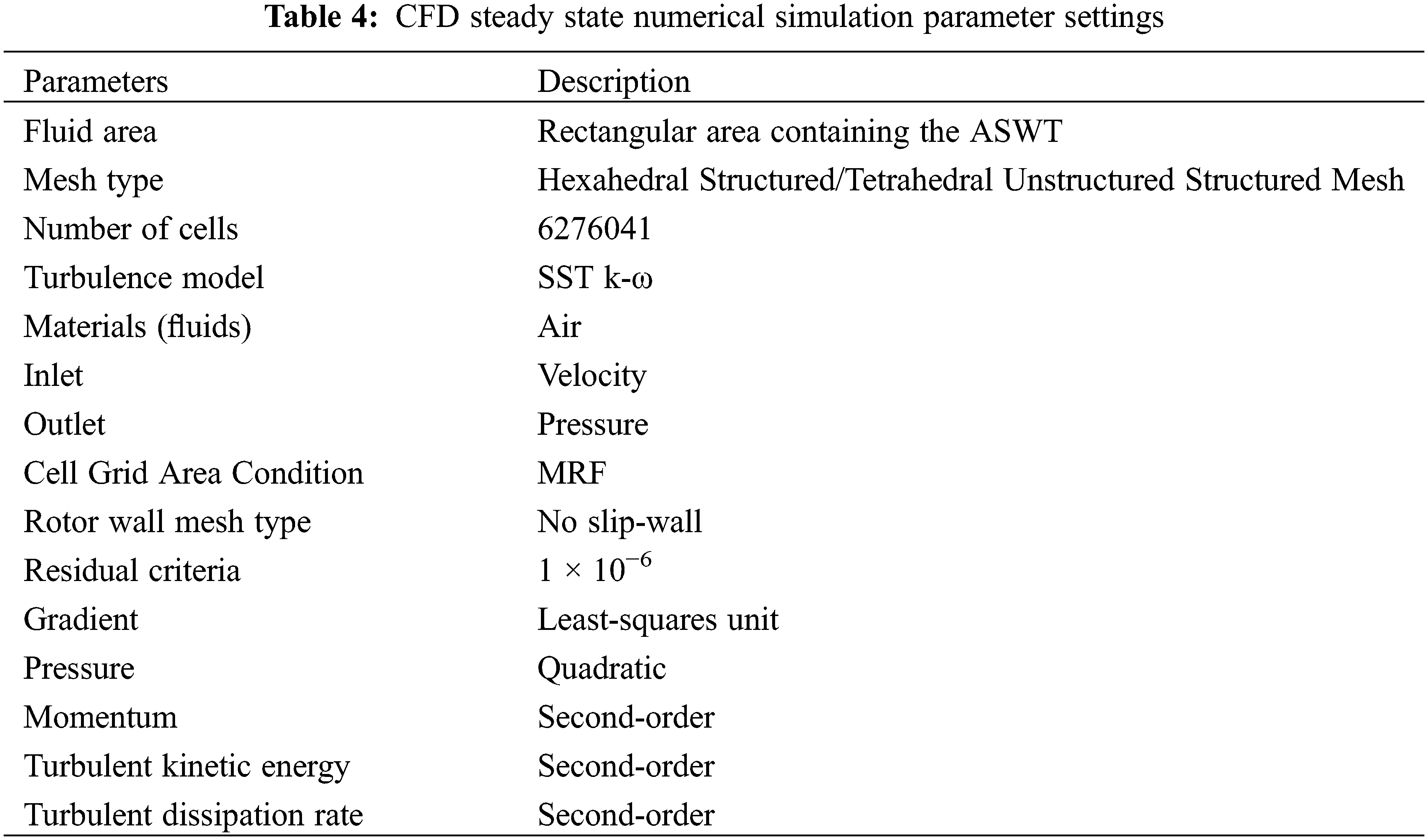
First, the steady-state solution is established by setting reference values for inlet velocity, windswept area, air density, and reference chord length to calculate torque and wind power coefficients. Second, the method employs the Coupled algorithm [19,28,29] using higher-order term relaxation to enhance the startup and general solution behavior of the flow simulation. The method couples pressure and velocity, and the spatial discretization gradient is based on the least squares cell. The convection and pressure terms are set to the second order. Since the rotational domain is a tetrahedral unstructured mesh, the momentum, turbulent kinetic energy, and turbulence dissipation rate are in the second-order windward format. The residuals are in the windward format. The convergence criterion is defined as 1 × 10⁻⁶. The detection point at the center of the rotation axis is defined to monitor the trend of the moment change. After about 200 iterations, it is observed that the monitoring value does not tend to be smoothed with the change in the number of iterative steps, and the residual curve steadily decreases to the vicinity of 1 × 10⁻⁶, indicating that the convergence condition is reached. The output of the steady-state flow results is torque. The steady-state computational parameter settings are shown in Table 4.
5.1 Aerodynamic Characterization
In this section, the primary focus is on the evaluation of the aerodynamic characteristics of the prototypical ASWT wind turbine and the improved ASWT.
5.1.1 Prototypical ASWT Aerodynamic Performance Evaluation
An error analysis of the actual measurement results is also a crucial step. Test errors may arise from imperfections in the test program, personal reading errors, instrument errors, and various other factors. Taylor’s theory is employed for the error analysis of the measurement results. The findings indicate that the relative errors of the torque coefficients at 10 and 8 m/s are 1.44% and 0.90%, respectively, and the errors of the power coefficients at 10 and 8 m/s are 98.56% and 99.1%, respectively.
where M is the measured result,
Here, the relative error is RE,
The prototypical ASWT is initially validated numerically at steady incoming wind speeds of 4, 6, 8, and 10 m/s. Figs. 8 and 9 illustrate the comparison between the experimental and numerically calculated results for CT and Cp, respectively. The results demonstrate a good agreement between the experimental values and the numerically calculated results in the corresponding TSR range at different wind speeds of 4, 6, 8, and 10 m/s.
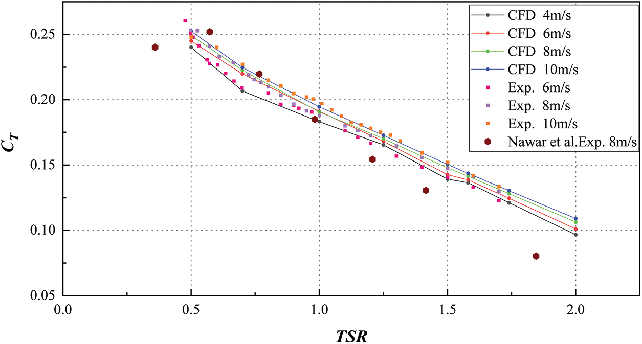
Figure 8: Experimental and numerical results of CT in different TSR ranges
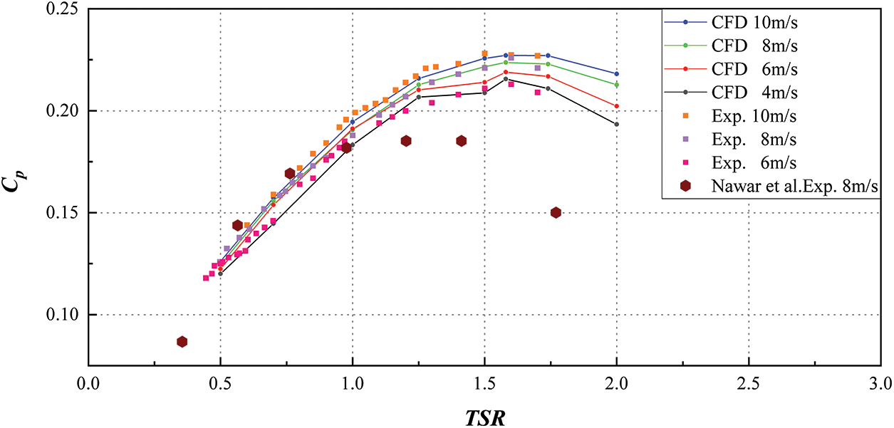
Figure 9: Experimental and numerical results of CP in different TSR ranges
The predicted values of CT and Cp were found to be slightly higher than those measured experimentally for the low wind conditions 6 and 8 m/s. To prevent the accumulation of excessive turbulent kinetic energy in the stagnation region, the SST k-ω turbulence model [30] is constrained by the use of the Kato-Launder limiter [26,30]. Under operating conditions with wind speeds up to 10 m/s, the numerical and experimental results agreed when the production limiting correction factor was applied. At high wind speeds of 10 m/s, where the Reynolds number reaches 2.47 × 10⁵, and the flow is in a fully developed turbulent state, the SST k-ω turbulence model alone is sufficient for accurate performance prediction of the ASWT.
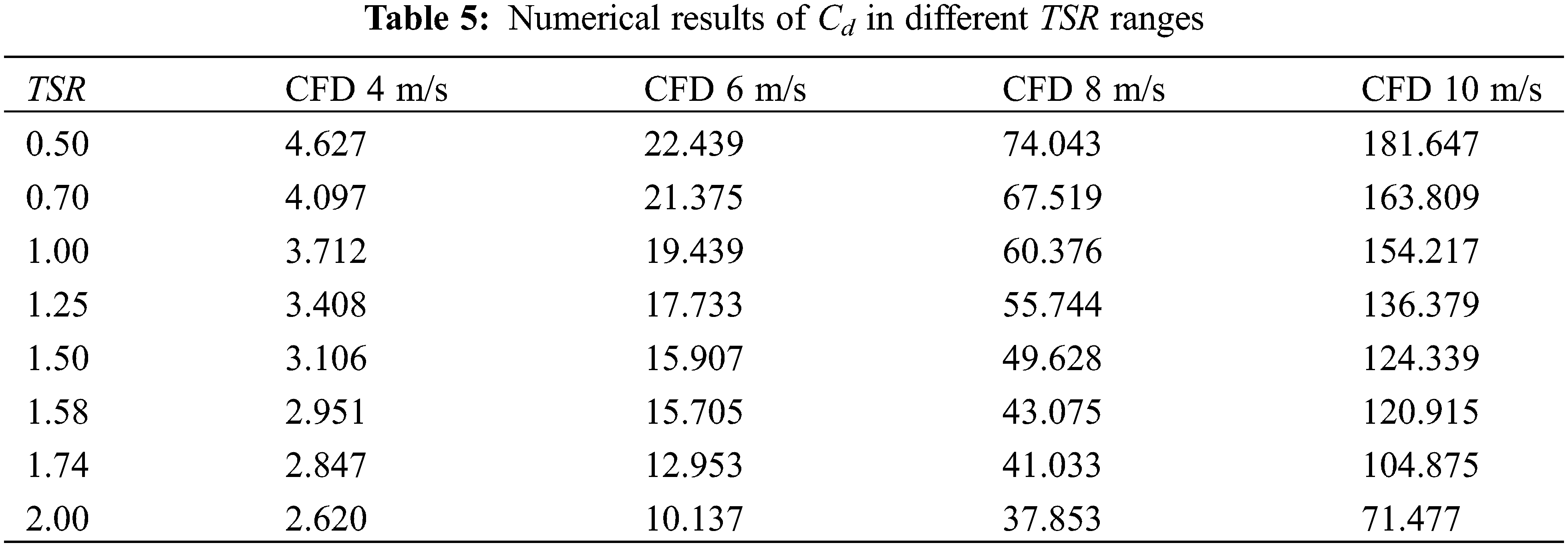
However, in the transition region with Reynolds numbers of 1.48 × 10⁵ and 1.98 × 10⁵ at wind speeds of 6 and 8 m/s, respectively, it is more appropriate to use the SST k-ω turbulence model with the Kato-Launder limiter. As shown in Fig. 8, numerical calculations reveal that the maximum values of CT are 0.244, 0.249, and 0.252 at TSR equal to 0.5 at wind speeds of 6, 8, and 10 m/s, respectively. Experimental results show slightly higher maximum values of CT at 0.260, 0.252, and 0.248 for the corresponding TSR under the same operating conditions. As shown in Fig. 9, the maximum values of CP are 0.219, 0.223, and 0.227 at TSR equal to 1.58, 1.58, and 1.58 when the wind speed is 6, 8, and 10 m/s, respectively. As a result, the maximum CP value is enhanced by 3.65% when the incoming wind speed is 8 and 10 m/s compared to the incoming wind speed of 6 m/s, and the maximum CP value is enhanced by 1.79% when the incoming wind speed is 10 m/s compared to the incoming wind speed of 8 m/s. The experimental results exhibit maximum values of CP at 0.213, 0.226, and 0.228 for the same operating conditions at TSR equal to 1.6, 1.6, and 1.5, respectively. Therefore, the maximum values of CP are enhanced by 7.04% when the incoming wind speed reaches 8 and 10 m/s compared to that at the incoming wind speed of 6 m/s. As shown in Fig. 8, the thrust coefficient decreases gradually with the increase of TSR due to the dominant role of torque in the case of fixed incoming wind speed. When the aerodynamic force in the X-direction increases gradually with the increase of incoming wind speed, the trend of thrust coefficient is significantly higher than that under low wind speed, and the overall trend remains the same, as shown in Table 5.
Under completely turbulent conditions, the ASWT exhibits unique peak-like curves that are plotted by the dimensionless parameters (CP, CT, TSR). These curves follow similar characterization principles as other wind turbine aerodynamic characteristics, showing distinct peaks unless there is a change in the flow pattern [31].
5.1.2 Effect of the Near-Wall Surface Function y+ on the Model
The boundary layer mesh height is specified according to the range of values of the dimensionless number y+ to ensure a reasonable range of y+ values for analyzing prototypical ASWT wind turbine models. The ASWT generates power by relying on both lift and drag to produce rotational motion. The results of numerical calculations comparing y+ < 3 and y+ < 1 are shown in Fig. 10. It is verified and discussed that the value of y+ < 1 is more suitable for the results of the experimental tests than the numerical case of y+ < 3.
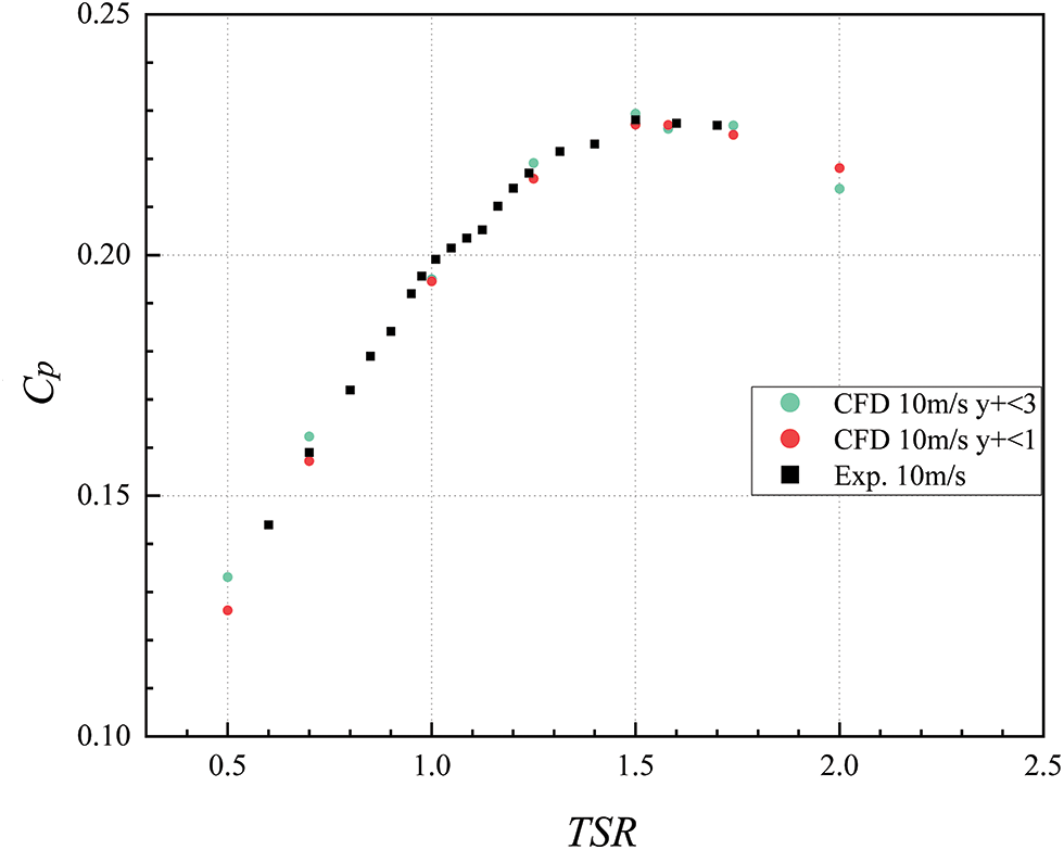
Figure 10: Experimental and numerical results of y+ for prototypical ASWT
5.1.3 Comparison of Retrofit Results Based on CFD Numerical Simulation Analysis
Under the premise of keeping y+ < 1,the improved ASWT is divided into eleven groups of blade models for numerical simulation and comparison. Three groups of the blade spread angles α1, α2, and α3 were grouped and numerically analyzed in the simulation. Firstly, the angle of α2 is discussed basded on α1 = 30°, α2 = 45°, α3 = 60°, and α2 varies in the ranges of 40°, 45°, 50°, 55°, while α1 and α3 remain constant at 30° and 60°, respectively. When α2 = 55°, the simulated range of TSR during the operation of this wind turbine is (0.5~3.0) and the CP reaches a maximum value of 0.263 when TSR is equal to 2, V = 10 m/s. Therefore, it is concluded that the optimal angle of α2 is 55°, as shown in Fig. 11a.
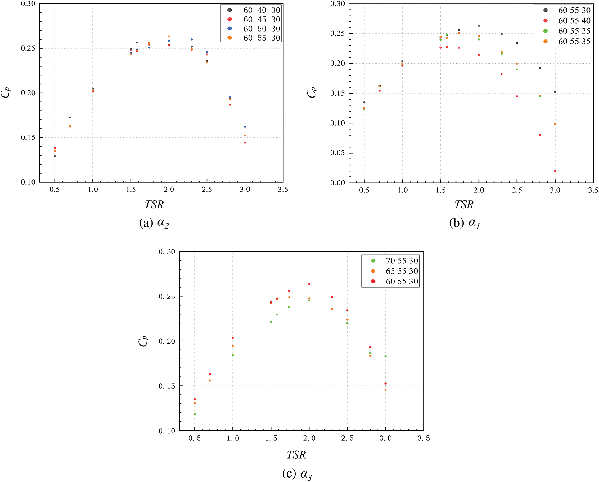
Figure 11: Effect of the spread angles: (a) α2, (b) α1, (c) α3 on CP values at V = 10 m/s
Under the same condition of wind speed V = 10 m/s, the effect of α1 on the CP value is analyzed, and α1 varies in the range of 25°, 30°, 35°, and 40°, while α3 and α2 are kept constant at 60° and 55°, respectively. A regular change of the data can be found in Fig. 11b, where α1 varies from the range of 25° to 40° with an initial increase and then a decrease in the CP value. At the same time, it validates Nawar et al. [22] designed the improved ASWT with the spread angles of α1 = 30°, α2 = 45°, and α3 = 60° for good aerodynamic performance. It is worth noting that changing the spread angle at the three sets of blades does not have any effect on the range of TSR. It can form a good interval of aerodynamic curves during the change of α1, and it also shows that ASWT was characterized by a wide speed range. When α1 = 30°, the TSR ranges from (0.5~3.0), and TSR is equal to 2, V = 10 m/s with CP reaches a maximum value of 0.263. Therefore, it is concluded that the optimum angle of α1 is 30°. α3 varies in the range of 60°, 65°, and 70°, and meanwhile, α1 = 30°, α2 = 55° are selected to keep the same as shown in Fig. 11c. It found that the variation of α3 has a more significant enhancement for the ASWT in the TSR range of (0.5~3.0) has a more significant enhancement. It is worth noting that reducing α3 from 70° to 60° finds that the aerodynamic performance in the TSR range of (0.5~3.0) is enhanced with the reduction of the angle and 60° is taken at α3 as the best.
Finally, it was concluded that the optimum blade spread angle of the improved ASWT was α1 = 30°, α2 = 55°, α3 = 60°. Fig. 12 shows the maximum CP of the improved ASWT is 0.263 at TSR = 2. In addition, the analysis of the figure shows that the TSR speed range of the improved ASWT is wider, and the maximum CP value of the improved ASWT is 17.93% higher than that of the prototypical ASWT. In addition, Fig. 13 summarizes the effect on the retrofitted ASWT under the variation of each parameter.
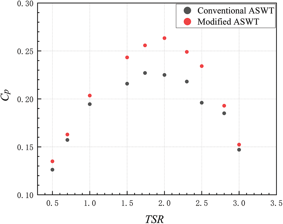
Figure 12: Comparison of the magnitude of the CP values of the improved ASWT and the prototypical ASWT
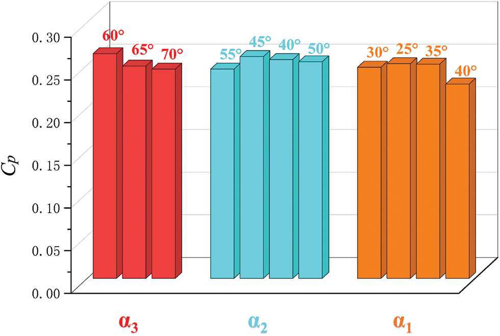
Figure 13: Effect of parameters on the maximum CP value of improved ASWT at V = 10 m/s
According to the design prototye, ASWT generates aerodynamic sources that are distributed in three dimensions. Therefore, it is particularly important to analyze the aerodynamic forces on the forward-looking datum. The aerodynamic analysis of the prototypical ASWT shown in Fig. 14 is performed by vector translation from the rotation axis to the tip area, C, U, and W represent the absolute velocity in the inflow direction, the linear velocity in the apical region, and the relative velocity synthesized from the absolute and linear velocities, respectively. β is between the absolute and relative velocities angle. The forces FX and FY generated in the incoming flow direction are decomposed into the lifting force FL and the drag force FD, FX can be decomposed into FLx, FDx, and FY can be decomposed into FLx, FDy. Therefore, the rotational motion of the ASWT is mainly dominated by FY. It is concluded that during the rotation of the ASWT. The three parts of the blades are arranged in alternating rows of 120°, so that the airflow is uniformly and repeatedly acted on each group of blades under the dominant effect of FY, thus achieving the purpose of power generation.
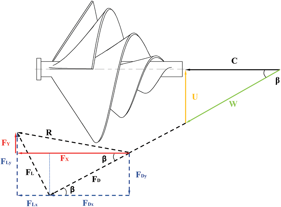
Figure 14: ASWT aerodynamic analysis
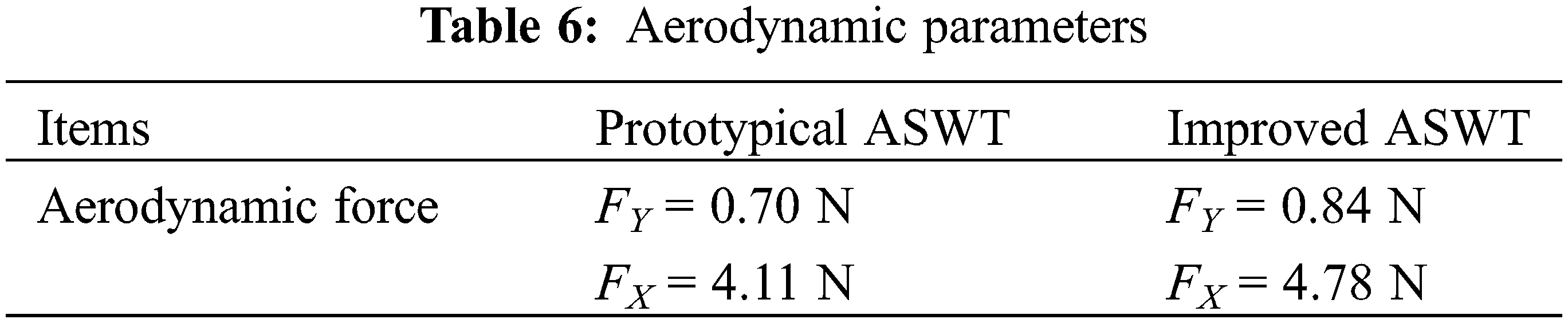
Table 6 shows the ASWT before and after the improvement when TSR is equal to 2, V = 10 m/s, with CP reaching its maximum value. The aerodynamic FY value of the prototypical ASWT is 0.70 N, and the aerodynamic FY value of the improved ASWT is 0.84 N. The FY value of the improvement is 20% higher than that of the prototypical ASWT. The aerodynamic FX value of the prototypical ASWT is 4.11 N, and the aerodynamic FX value of the improvement ASWT is 4.78 N. The FX value of the modification is 16.3% higher than that of the prototypical ASWT.
5.1.4 Characterization of the Flow Field
In this paper, the study of the velocity flow field and pressure field contours can effectively help to understand the effect of ASWT on aerodynamic performance before and after the modification. At TSR = 2, V = 10 m/s, Figs. 15a, 15b reveal the comparison of velocity and pressure contours of prototypical and improved ASWT, respectively. When the turbulent kinetic energy starts to impinge on the surface of the blades, it generates different When the turbulent kinetic energy starts to flow into the blade surface, different high and low-pressure regions in the windward and leeward directions of the incoming velocity. With the improvement of the blade, the high-pressure region is shifted from the second and third blades before the improvement to the first and second blades after the modification, and the low-pressure region is also smaller with the modification.
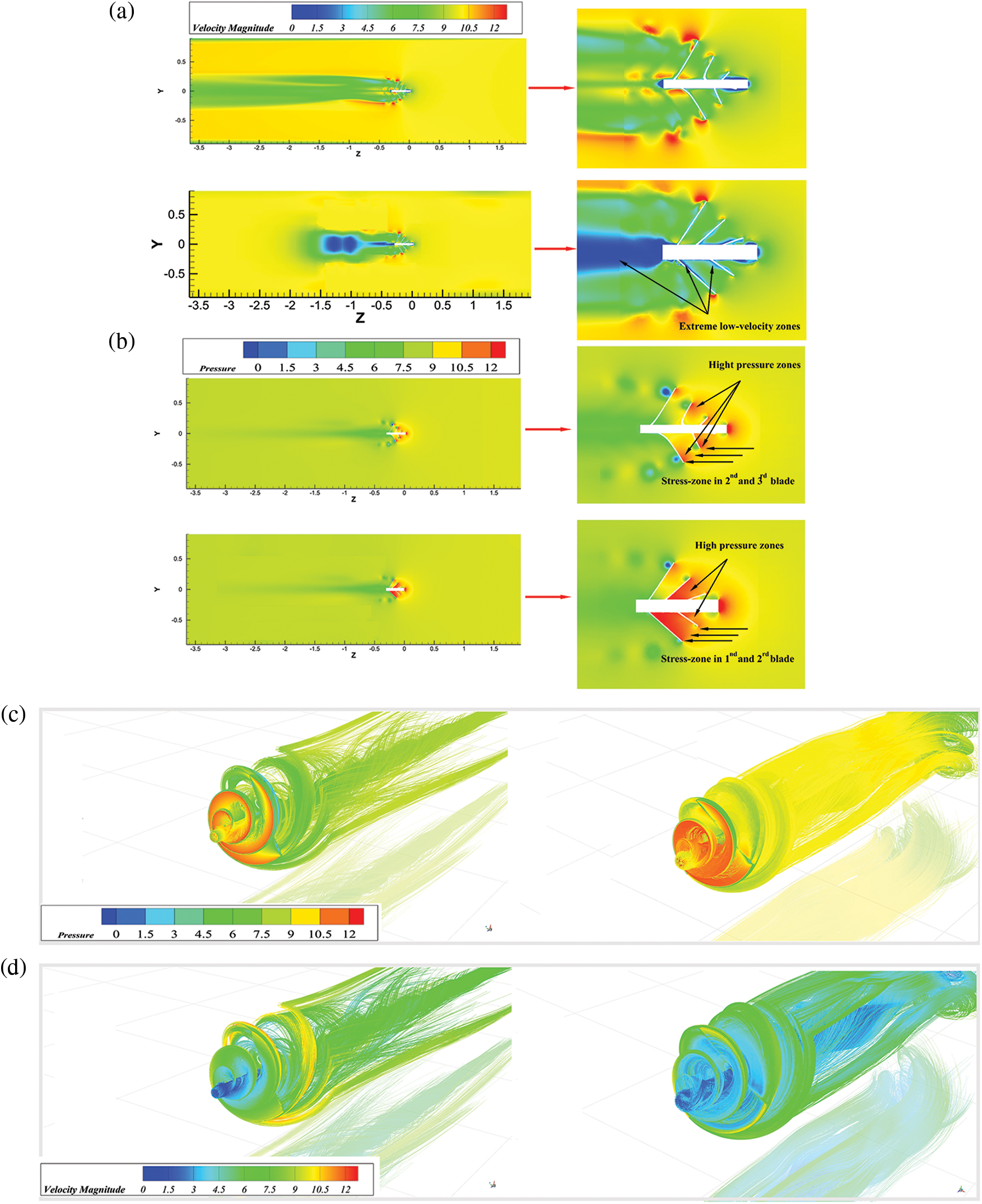
Figure 15: (a) Velocity contours comparing the prototype and modification, (b) Pressure contours comparing the prototype and modification, (c) Pressure contours comparing the flow streamline distribution of the prototype and modification, (d) Velocity contours comparing the flow streamline distribution of the prototype and modification
As shown in Fig. 11, the improved ASWT as α1 decreases in the range of (35° to 30°) and the blade spread angle α2 increases in the range of (40° to 45°), as in Figs. 15a and 15c. Therefore, a certain high-pressure region is formed upstream of the spread angles α1, α2 at the first and second blades. The formation of a corresponding low-pressure region downstream of the blades is conducive to the improvement of the ASWT’s ability to capture wind energy. As shown in Figs. 15b and 15d, the comparison of the velocity contours and flow field streamlines found that the improved ASWT forms an extremely low-velocity region in the downstream region of the incoming wind speed, implying that more efficiency can be obtained when the improved ASWT operates in comparison with the prototypical ASWT, which is verified with each other and with the analysis of the above results.
The aerodynamic performance of the prototypical ASWT and the improved ASWT was investigated. Using CFD modeling, a variable angle structure was applied to the ASWT, and the effects of different blade structure changes on the aerodynamic performance of the ASWT under the optimal aerodynamic performance were evaluated. The main conclusions are as follows: The numerical calculations in the operating range of the total leaf tip speed ratio are consistent with the comparison of the test results.
1. When the airflow through the ASWT reaches a Reynolds number of 2.47 × 10⁵, indicating fully developed turbulence, with a rotor radius of 35 mm and wind speed of 10 m/s, experimental results show that for incoming wind speeds of 6, 8, and 10 m/s, and TSR of 1.6, 1.6, and 1.5, the maximum values of the CP are 0.213, 0.226, and 0.228, respectively.
2. Based on the flow field analysis, the second blade was found to have a dominant role in influencing the aerodynamic performance of the ASWT in the Z-axis coordinate equivalent plane. The best aerodynamic performance of the retrofitted ASWT was attained when α1 = 30°, α2 = 55°, and α3 = 60°. At a wind speed of 10 m/s, the aerodynamic performance of the improved ASWT is 15.99% higher than that of the prototypical ASWT. The relative errors of the experimental and simulated values are 1.44% and 0.90% for wind speeds of 10 and 8 m/s, respectively, and the torque coefficient measurement accuracies are 98.56% and 99.10%, respectively.
Our research is an effective supplement to the existing research. It has good reference significance, which can provide reference and reference for ASWT performance research, experimental optimization design, and performance prediction. In the future, the airfoil-related parameters will be applied to the ASWT to compare the optimization of its aerodynamic performance and the optimization of the acoustic propagation law.
Acknowledgement: None.
Funding Statement: This study was supported by the National Natural Science Foundation of China. Project under Grant (Nos. 51966018 and 51466015).
Author Contributions: The authors confirm contribution to the paper as follows: supervision, project administration, funding acquisition and writing-review & editing: Yuanjun Dai, Zetao Deng, Baohua Li; study conception and design: Zetao Deng; experiment and data collection: Zetao Deng, Lei Zhong, Jianping Wang; analysis and interpretation of results: Zetao Deng, Lei Zhong, Jianping Wang; draft manuscript preparation: Zetao Deng. All authors reviewed the results and approved the final version of the manuscript.
Availability of Data and Materials: Since more comparative studies will be conducted in the future, the authors hope that the data will be publicly displayed after the research field and research content are further broadened. The authors do not have permission to share data.
Conflicts of Interest: The authors declare that they have no known competing financial interests or personal relationships that could have appeared to influence the work reported in this paper.
References
1. Hu Y, Bu SQ, Luo JQ, Wen JX. Generalization of oscillation loop and energy flow analysis for investigating various oscillations of renewable energy systems. Renew Energ. 2023;218:119352. [Google Scholar]
2. Michael WJ, Maximilian H, Jan G, Tom T, Julian S, Patrick K, et al. Global LCOEs of decentralized off-grid renewable energy systems. Renew Sust Energ Rev. 2023;183:1–2. [Google Scholar]
3. Armin A, Li W, Sandberg OJ, Xiao Z, Ding LM, Nelson J, et al. A history and perspective of non-fullerene electron acceptors for organic solar cells. Adv Energy Mater. 2021;11(5):1–2. [Google Scholar]
4. Maria S, Pei H, Chris B, Erik D. Evaluation of hosting capacity of the power grid for electric vehicles—a case study in a Swedish residential area. Energy. 2023;284:129293. [Google Scholar]
5. Yang SY, Gao HO, You FQ. Integrated optimization in operations control and systems design for carbon emission reduction in building electrification with distributed energy resources. Appl Energy. 2023;284:100144. [Google Scholar]
6. Kishwar A, Du J, Dervis K, Judit O, Satar B. Do environmental taxes, environmental innovation, and energy resources matter for environmental sustainability: evidence of five sustainable economies. Heliyon. 2023;9(11):e21577. [Google Scholar]
7. Liu Y, Li YP, Huang GH, Lv J, Zhai XB, Li YF, et al. Development of an integrated model on the basis of GCMs-RF-FA for predicting wind energy resources under climate change impact: a case study of Jing-Jin-Ji region in China. Renew Energ. 2023;219:119547. [Google Scholar]
8. Liu X, Lu C, Li GQ, Godbole A, Chen Y. Effects of aerodynamic damping on the tower load of offshore horizontal axis wind turbines. Appl Energy. 2017;204:1101–14. [Google Scholar]
9. Jan K, Chen J, Junhua W, Yang HX, Fu WN. A novel magnetic levitated bearing system for vertical axis wind turbines (VAWT). Appl Energy. 2012;90(1):148–53. [Google Scholar]
10. Ahmad H, Amne E, Michel E. Numerical investigation of the use of flexible blades for vertical axis wind turbines. Energy Convers Manag. 2024;299:117867. [Google Scholar]
11. Bai HM, Wang NN, Wan DC. Numerical study of aerodynamic performance of horizontal axis dual-rotor wind turbine under atmospheric boundary layers. Ocean Eng. 2023;280:114944. [Google Scholar]
12. Zhang TT, Elsakka M, Huang W, Wang ZG, Ingham DB, Ma L, et al. Winglet design for vertical axis wind turbines based on a design of experiment and CFD approach. Energy Convers Manag. 2019;195:712–26. [Google Scholar]
13. Zhang TT, Wang ZG, Huang W, Ingham D, Ma L, Pourkashanian M. A numerical study on choosing the best con fi guration of the blade for vertical axis wind turbines. J Wind Eng Ind Aerodyn. 2020;201:9–10. [Google Scholar]
14. Hameed HSA, Hashem I, Nawar MAA, Attai YA, Mohamed MH. Shape optimization of a shrouded Archimedean-spiral type wind turbine for small-scale applications. Energy. 2023;263:125809. [Google Scholar]
15. Hossam H, El Maksoud Rafea Mohamed ABD. A comparative examination of the aerodynamic performance of various seashell-shaped wind turbines. Heliyon. 2023;9(6):e17036. [Google Scholar]
16. Chaudhary S, Shubham J, Nanda RK, Saurabh P, Parmod K, Dhar V, et al. Comparison of torque characteristics of archimedes wind turbine evaluated by analytical and experimental study. Int J Mech Prod Eng. 2016;4(8). [Google Scholar]
17. Rao SS, Shanmukesh K, Naidu MK, Kalla P. Design and analysis of archimedes aero-foil wind turbine blade for light and moderate wind speeds. Int J Recent Technol Mech Electr Eng. 2018;5(8). [Google Scholar]
18. Song K, Huiting H, Yuchi K. Aerodynamic performance and wake characteristics analysis of archimedes spiral wind turbine rotors with different blade angle. J Energies. 2022;16(1):385. [Google Scholar]
19. Kamal Ahmed M, Nawar Mohamed AA, Attai Youssef A, Mohamed Mohamed H. Archimedes spiral wind turbine performance study using different aerofoiled blade profiles: experimental and numerical analyses. Energy. 2023;262:1–2. [Google Scholar]
20. Kazem S, Gholamhassan N, Rizalman M, Fairusham GM, Ei-Shafy AS, Mohamed M. Introducing a design procedure for archimedes screw turbine based on optimization algorithm. Energy Sustain Dev. 2023;72:162–72. [Google Scholar]
21. Zhang D, Penghua G, Qiao H, Jingyin L. Parametric study and multi-objective optimization of a ductless archimedes screw hydrokinetic turbine: experimental and numerical investigation. Energy Convers Manag. 2022;273:116423. [Google Scholar]
22. Nawar MAA, Abdel Hameed HS, Ramadan A, Attai YA, Mohamed MH. Experimental and numerical investigations of the blade design effect on archimedes spiral wind turbine performance. Energy. 2021;223:4–5. [Google Scholar]
23. Quan H, Zhang T, Xu H, Luo S, Nie J, Zhu X. Photo-curing 3D printing technique and its challenges. Bioact Mater. 2020;5(1):110–5. [Google Scholar] [PubMed]
24. Bachant P, Wosnik M. Effects of reynolds number on the energy conversion and near-wake dynamics of a high solidity vertical-axis cross-flow turbine. Energies. 2016;9(2):8–11. [Google Scholar]
25. Coughtrie AR, Borman DJ, Sleigh PA. Effects of turbulence modelling on prediction of flow characteristics in a bench-scale anaerobic gas-lift digester. Bioresour Technol. 2013;138:297–306. [Google Scholar] [PubMed]
26. Menter Florian R. Two-equation eddy-viscosity turbulence models for engineering applications. AIAA Journal. 1994;32:1598–605. [Google Scholar]
27. Bastian N. OpenFOAM: a tool for predicting automotive relevant flow fields. Division of Fluid Dynamics, Department of Applied Mechanics, Chalmers University of Technology: Sweden; 2020. [Google Scholar]
28. Mehran M, Mojtaba T, Hossein NM, Narek B. Optimization of airfoil based savonius wind turbine using coupled discrete vortex method and salp swarm algorithm. J Clean Prod. 2019;222:47–56. [Google Scholar]
29. He KP, Ye JH. Dynamics of offshore wind turbine-seabed foundation under hydrodynamic and aerodynamic loads: a coupled numerical way. Renew Energ. 2023;202:453–69. [Google Scholar]
30. Kato M, Brian L. The modelling of turbulent flow around stationary and vibrating square cylinders. In: Proceedings of the 9th Symposium on Turbulent Shear Flows, 1993; Kyoto, Japan. [Google Scholar]
31. Peter B, Martin W. Effects of reynolds number on the energy conversion and near-wake dynamics of a high solidity vertical-axis cross-flow turbine. Energies. 2016;9(2):73. [Google Scholar]
Cite This Article
 Copyright © 2024 The Author(s). Published by Tech Science Press.
This work is licensed under a Creative Commons Attribution 4.0 International License , which permits unrestricted use, distribution, and reproduction in any medium, provided the original work is properly cited.
 Downloads
 Citation Tools