Coupled CFD-DEM Numerical Simulation of the Interaction of a Flow-Transported Rag with a Solid Cylinder

1  Introduction

In the realm of fluid dynamics, the flow around bluff bodies is a prevalent research topic with practical engineering applications in fields such as aviation, aerospace, marine, and defense. Among these, the flow around a cylinder exemplifies a typical bluff body flow, where the cylindrical geometry obstructs the fluid flow and generates distinct forces in various directions. The resulting flow field exhibits strong nonlinearity and uncertainty, impacting the stability of the geometry. Therefore, investigating the flow characteristics around cylinders holds substantial theoretical and practical significance.

Researchers have extensively analyzed the flow characteristics around cylinders. Some scholars, such as Zobeyer et al. [1], have used experimental approaches to explore the effects of different center distances on the mean and turbulent flow profiles around cylinders. Kim et al. [2] experimentally investigated the dynamics of a cylinder arranged between two sidewalls in a uniform flow.

Alternatively, other scholars have opted for numerical simulation methods to investigate flows around cylinders. Vinodh et al. [3] studied the dynamics between two closely spaced cylinders. Zhao et al. [4,5] numerically analyzed flow models of a cylinder at different Reynolds numbers to find that the length of the wake region and the turbulence intensity increase with the Reynolds number of the incoming flow. Afroz et al. [6] conducted a numerical study on laminar cross-flow over a cylinder with smooth and longitudinal groove surfaces. Ali et al. [7] investigated the impact of arrangement of two cylinders on their flow-induced vibrations (FIV) and heat transfer behavior at a Reynolds number of 100, while Mahbub et al. [8] studied the effects of different non-parallel tandem cylinder arrangements on flow states. Rajpoot et al. [9] numerically explored various cylinder-to-wall gap ratios (0.1 ≤ G/D ≤ 4.0) and inter-cylinder spacing ratios (0.5 ≤ S/D ≤ 8.0), at a certain Reynolds number (Re) = 100. Lee et al. [10] investigated the effectiveness of installing small control rods upstream of a cylindrical body. Other scholars have conducted research from a theoretical perspective. For instance, Wang et al. [11] conducted a detailed study on the ISW forces acting on a cylinder using a three-dimensional numerical wave tank and the large-eddy simulation (LES) method.

Currently, research on flows around cylinders predominantly center on the pure liquid phase, with relatively few numerical investigations involving both liquid and solid phases. Huang et al. [12,13] conducted numerical simulations on the dispersion distribution of particles in the wake of a sparse liquid-solid two-phase flow around a cylinder. Wei et al. [14] used a computational fluid dynamics (CFD) method to study the mechanism of tip leakage vortex and energy loss caused by pump cavitation. Li et al. [15] numerically simulated large particle solid-liquid two-phase flows and wall wear in curved pipes with different wall shapes.

While the combined computational fluid dynamics and discrete element method (CFD-DEM) approach is widely adopted for numerical simulations of solid-liquid two-phase flows, studies have mainly focused on spherical particles or slender structural fibers, neglecting square fibers like rags. Therefore, this study aims to investigate the motion of rags in the flow around a cylinder, considering factors such as bending and stretching of the fabric during motion. Based on the CFD-DEM method, a new improved Hertz Mindlin (no slip) model is proposed, incorporating parameters such as shear strength, normal strength, normal stiffness per unit area, and shear stiffness per unit area. To verify the feasibility of the proposed numerical model, simulation data are compared with experimental data.

2  CFD-DEM Coupling Method

The CFD-DEM method is a combination of CFD and DEM techniques. In the CFD-DEM method, liquid is regarded as a continuous phase and particles are regarded as a discrete phase. In the calculation process, the continuous medium is controlled by a continuity equation and momentum by a Navier-Stokes equation. The discrete phase, which is more challenging to compute, is the focus of this study.

Coupling between the continuous phase and discrete phase is mainly accomplished by the two-way exchange of momentum and mass. A flow chart of this process is shown in Fig. 1 [16].

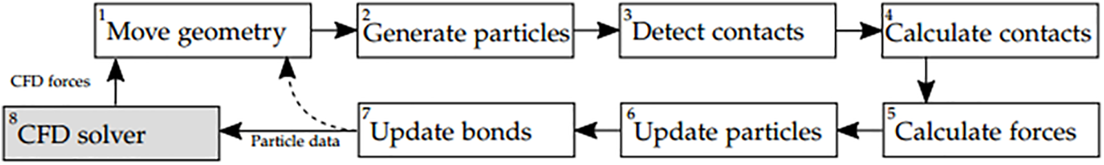
Figure 1: Overview of an iteration in EDEM when coupling to ANSYS Fluent

2.1 Continuous Phase Control Equation

The fluid flow in the sink is governed by the principles of mass conservation, momentum conservation, and energy conservation. Given the negligible impact of heat exchange and temperature changes on the water tank, and considering the fluid medium as incompressible, it is sufficient to focus on the simplified mass conservation (Eq. (1)) and momentum conservation (Eq. (2)):

∂ui∂xi=0, (1)

∂(ρui)∂t+∂(ρuiuj)∂xj=∂τij∂xj−6πμa(u−up), (2)

where t is time, ρ is the fluid density, u is the fluid velocity, up is the particle velocity, a is the particle radius, and μ is the fluid dynamic viscosity. The variable τ is the total stress tensor, which is expressed as:

τij=−pδij+μ(∂ui∂xj+∂uj∂xi), (3)

where p is the fluid pressure.

2.2 Discrete Phase Control Equation

To better analyze the forces acting on particles in a cylindrical flow, the forces can be categorized based on their distinct modes of action into three groups: forces unrelated to the relative motion between the fluid and particles (e.g., gravity, inertia force, and pressure gradient); forces caused by the relative motion between particles and fluids in the direction of particle motion velocity (e.g., drag force, virtual mass force, and Basset force); and forces arising from the relative motion between particles and fluids, but acting perpendicular to the relative motion direction (e.g., Magnus forces and Safhmn forces).

Due to the small velocity gradient in the mainstream region of the flow field and the particle size less than 5 mm, the virtual mass force, Safhmn lift, and Magnus lift forces acting on solid particles are excluded from consideration in this simulation. It is assumed that particles primarily experience gravity, inertial forces, pressure gradient forces, drag, and Basset forces, as well as contact forces between particles. The resulting motion equation for solid particles is:

mpd2xpd2t=Fc+Fp+Fg+Fin+Fr+FB, (4)

where mp is the mass of the particle and xp is the translational displacement. Fc ,  Fp , Fg , Fin , Fr , and  FB represent contact force, pressure gradient force, gravity, inertial forces, drag, and Basset forces, respectively.

Unlike the rigid particle two-phase flow model, the flexible impurity two-phase flow model comprises multiple particle models arranged in a row, with contact between particles. Therefore, it is necessary to consider the contact force between particles, primarily consisting of normal and tangential contact forces (Fig. 2a). The following section provides mainly a detailed introduction to the contact force between particles.

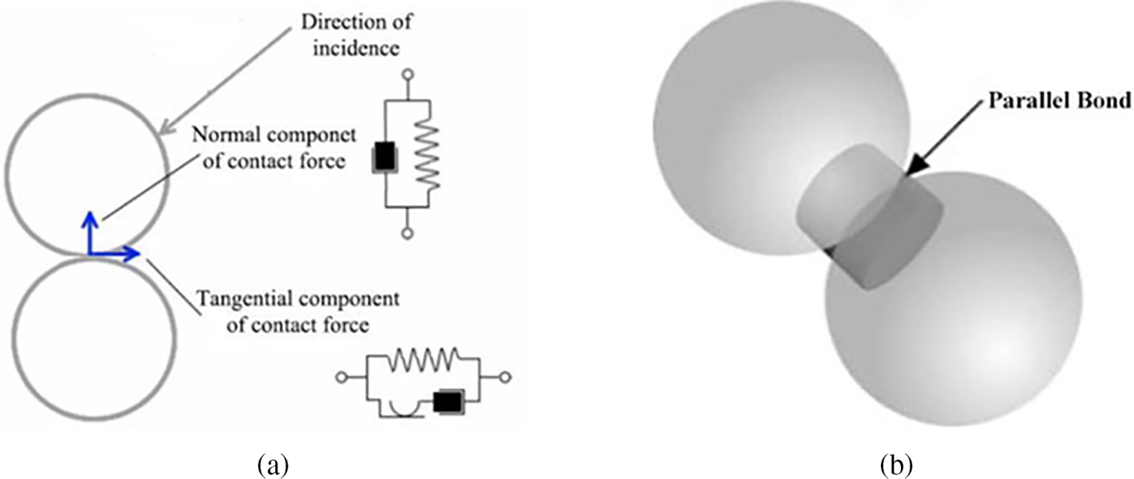
Figure 2: Particle connection diagram. (a) DEM particle contact model (b) Granular binding

The Hertz-Mindlin non-slip model can be used to calculate the particle contact force. This contact model is a variant of the nonlinear spring-damper contact model [17], as shown in Fig. 2a. The contact force is determined as follows:

Fc=Fn+Ft, (5)

where Fn denotes the normal contact force, and the normal contact is replaced by the combined action of a spring and damper. As depicted in Fig. 2a, the spring reflects the stiffness of the material in the normal direction (Young’s modulus), while the damper represents the normal recovery. Thus, the normal contact force Fn is defined as:

Fn=−Kndn−Nnυn, (6)

where Kn is the normal elastic coefficient, dn represents the normal displacement between particles, Nn is the normal damping coefficient, and vn denotes the normal relative velocity between particles.

The tangential contact force Ft  is replaced by the combined action of a spring, damper, and slider. As shown in Fig. 2a, the spring reflects the stiffness of the material in the tangential direction (Young’s modulus), while the damper represents the tangential recovery and the slider represents the friction. The normal contact force Ft is defined as follows:

Ft=−Ktdt−Ntυt, (7)

where Kt represents the tangential elastic coefficient, dt is the tangential displacement between particles, Nt is the tangential damping coefficient, and υt indicates the tangential relative velocity between particles.

The particles are connected by massless bonds, as illustrated in Fig. 2b.

2.3 Rag Model Structure

The soft sphere model simplifies the normal force between particles into springs and dampers, and the tangential force into springs, dampers, and sliders. Accordingly, its application allows for the creation of more intricate particle models, including shapes like bending and folding. In this simulation, the particle cluster model is employed to group particles and transform them into complex shapes, as shown in Fig. 3. Displacement coordinates are recorded at points located at the top, middle, and bottom of the model.

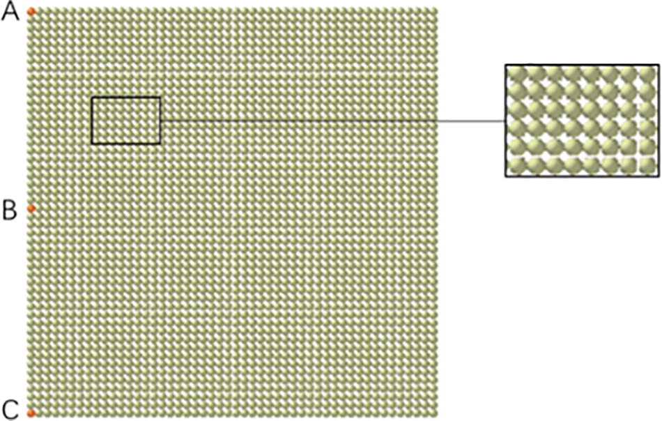
Figure 3: Particle model

The particles constituting the rag have a radius of 1 mm, and the contact radius is 1.2 mm. The size of the rag used in the simulation is 100 mm × 100 mm, resulting in a configuration with 50 particles × 50 particles. The density of spherical particles is 2500 kg/m3, Poisson’s ratio is 0.25, and the shear modulus is 1 × 108 Pa.

3  Experimentation

To verify the proposed method’s feasibility, the model calculation results were compared with erosion wear experimental data for a right angle bend provided by Baker Petroleum Tools Company, USA [18]. The simulated right angle bend (Fig. 4) has a pipe diameter of D = 25.4 mm, with the upstream pipeline L1 extending 16 times the pipe diameter and the downstream pipeline L2 extending 20 times the pipe diameter. The computational area was divided into zones, utilizing a hexahedral structured grid throughout. In the experiment, both the upstream and downstream lengths of the right angle bend were 140.589 mm, and liquid water was used as the conveying medium with fluid velocities of 15.24 and 26.15 m/s, respectively. The solid particles are semi-circular quartz sand with a diameter of 256 μm and a mass flow rate of 0.077 kg/s. The pipe wall material is Inconel718.

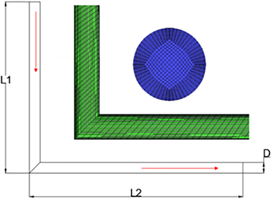
Figure 4: The geometric structure and grid diagram of a right-angle bend

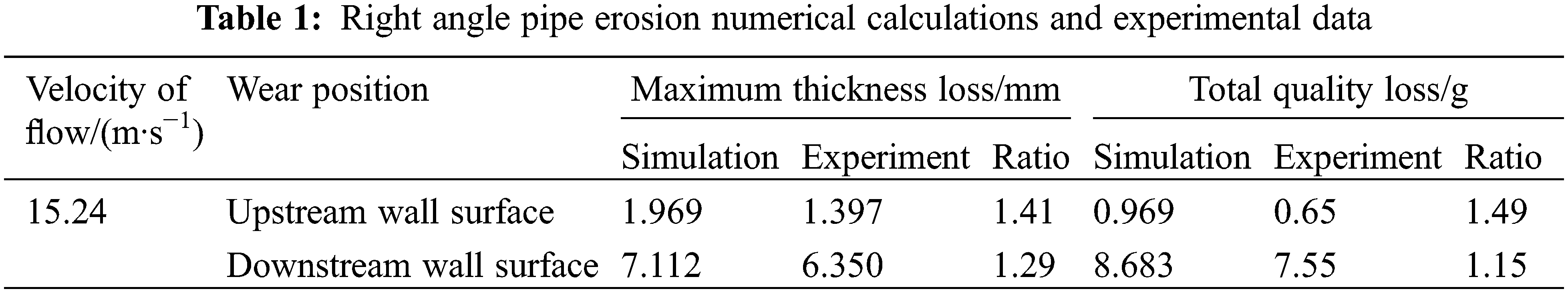
According to the wear chart (Fig. 5), the maximum wear position on the upstream pipe wall is located on the inner side of the 90° angle, resulting from the direct impact of solid particles carried by the fluid. The maximum wear position of the downstream pipe wall occurs on the inner side of the pipe wall, a distance away from the bending angle. Both positions are consistent between the numerical and experimental results. The numerical calculation results of the overall mass loss and maximum wear thickness are generally larger than the experimental results (Table 1), with errors within 1.5 times.

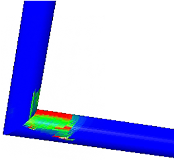
Figure 5: Erosion distribution diagram of right angle bend at 15.24 m/s

The model is capable of accurately predicting the location of maximum wear on the right angle pipe, affirming the feasibility of the proposed method. Building on this foundation, the consideration of connection forces between particles is crucial for accurately simulating the behavior of the rag.

4  Numerical Simulation

4.1 Tank Structure

Interactions between flexible 2D rags and fixed 3D cylindrical obstacles, ignoring gravity, are taken into account in this simulation. The rag is transported in a rectangular channel flow and initially located perpendicular to the flow direction. The initial shape of the sink is shown in Fig. 6. The size of the sink is 0.45 m × 0.2 m × 0.2 m, the diameter of the cylinder is 0.05 m, the distance from the center of the cylinder to the upstream area is 0.2 m, the distance to the downstream area is 0.2 m, the distance to the lower wall is 0.08 m, and the distance to the upper wall is 0.12 m.

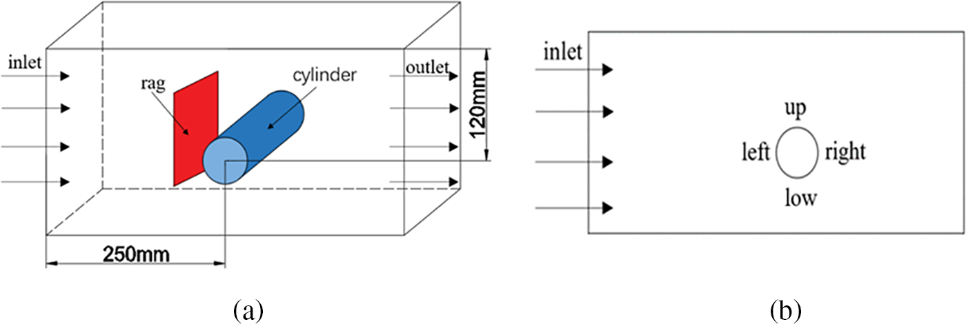
Figure 6: Water tank model. (a) Three-dimensional diagram (b) Cross section

4.2 Mesh and Boundary Conditions

The computational fluid domain uses hexahedral structured mesh. Grid independence verification was conducted on the model to reduce the influence of the number of grids on the numerical solution. Table 2 shows the variations in drag coefficient (Cd) and lift coefficient (Cl) with the number of grids. The drag coefficient reflects the degree of obstruction of the fluid to the motion of an object, while the lift coefficient reflects the vertical upward force generated by the fluid on the object. The hydrodynamic effects on a cylinder can be evaluated through these two coefficients. In this case, increasing the number of grids beyond 1001286 has a negligible imapact on the calculation results. Therefore, the chosen grid count is 1001286. The grid division is depicted in Fig. 7.

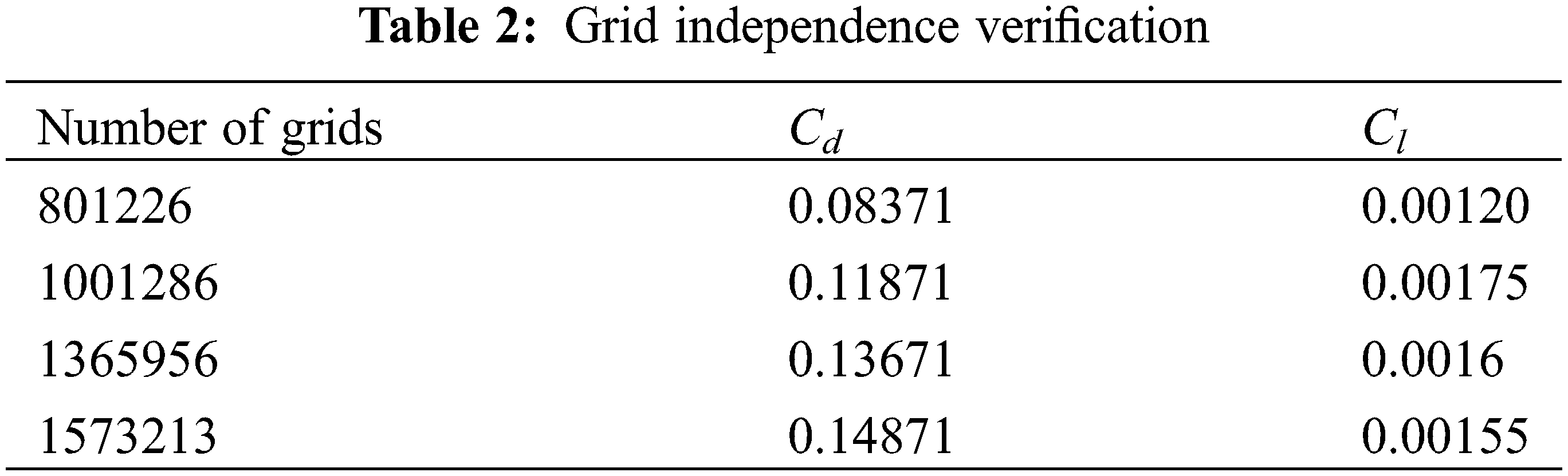
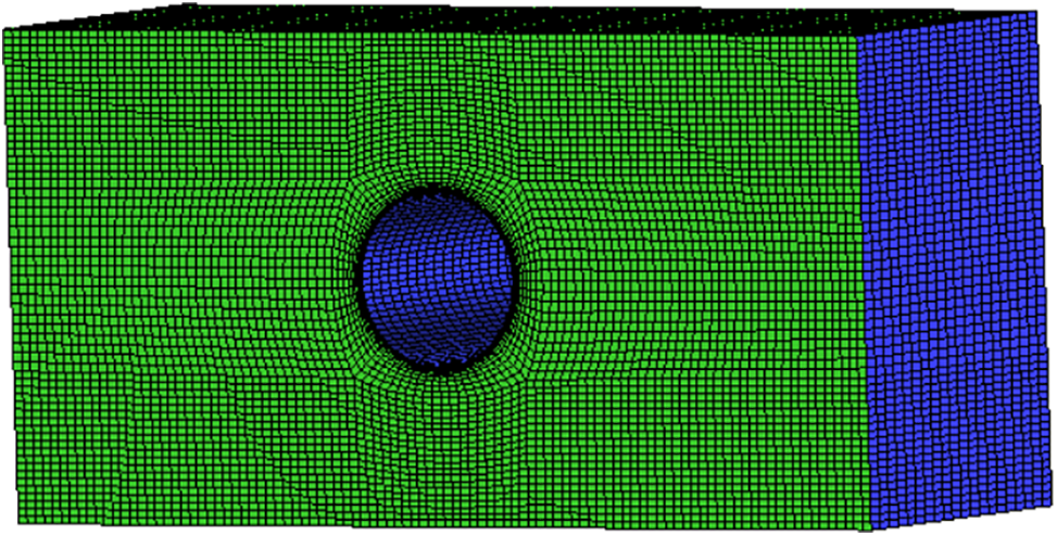
Figure 7: Schematic diagram of grid division

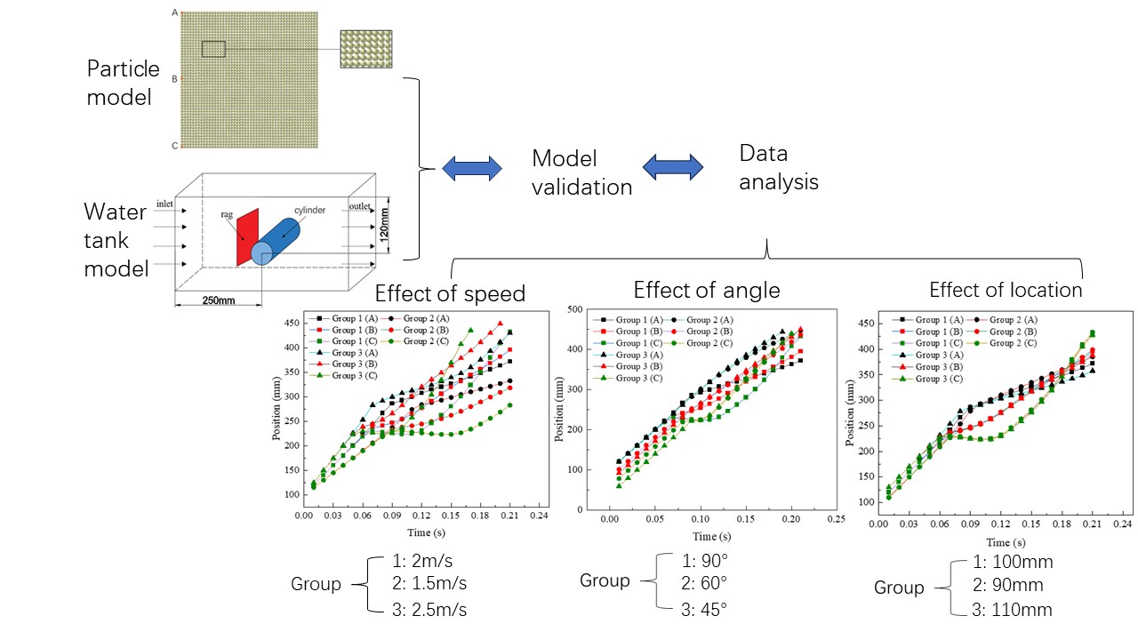
The trajectory of a rag in a water tank and the influence of different factors on its trafficability was simulated with the CFD-DEM method. Table 1 outlines seven schemes established for this analysis, each with distinct conditions. In FLUENT, the velocity inlet and pressure outlet were selected as the boundary conditions for calculation. The SIMPLE method in pressure-velocity coupling was chosen as the numerical calculation scheme. The structure is relatively simple, so the relevant requirements were satisfied by setting the momentum, turbulent kinetic energy, and turbulent dissipation rate as first-order upwind. All walls were set as non-slip boundaries.

Real-time data transmission is essential for accurate coupling calculation results. To satisfy this requirement, FLUENT was operated with transient calculation processes. The time step in FLUENT, in accordance with the necessary integer multiple of 10–100 with the time step in EDEM, was set to 1.0 × 10−4 s with an EDEM time step of 5.0 × 10−6 s. The Reynolds numbers were 75000, 100000, and 125000 for groups with velocities of 1.5, 2, and 2.5 m/s, respectively.

5  Results and Analysis

5.1 Rag Movement Track at Different Time Points

The trajectory of Group 1 (2 m/s, 90°, 100 mm) was analyzed to begin the analysis. The evolution at six consecutive instants is illustrated in Fig. 8. Initially, before contact with the cylinder, the rag moves linearly in the fluid. Upon contact, the middle part of the rag halts on the cylinder’s surface while its ends continue to move in the fluid direction. Subsequently, propelled by the upper end, the rag ascends along the cylinder as a whole. Finally, after passing over the cylinder, the rag continues to move downstream in the channel propelled by the fluid.

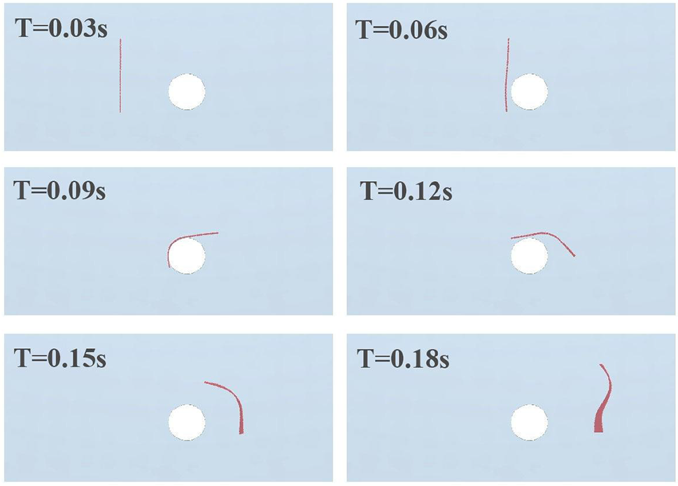
Figure 8: Fragments at different time points during collision

The time point at 0.09 s was isolated for a closer examination of pressure and velocity distributions during rag-cylinder contact. The velocity and pressure distributions at 0.09 s are shown in Figs. 9 and 10, respectively. As shown in Fig. 9, the fluid velocity is lower on the left side of the cylinder due to contact with the rag, creating smaller vortices on the right side. Velocity gradually increases with distance. The distance between the upper and lower regions of the cylinder influences fluid velocity; as it decreases, the fluid velocity in these regions increases. Simultaneously, the velocity in the upper region of the rag surpasses that in the lower region, propelling the rag forward. As illustrated in Fig. 10, the pressure is mainly concentrated in the contact area between the rag and the cylinder. Negative pressure forms in the upper and lower areas of the cylinder, with lower pressure in the lower area compared to the upper area.

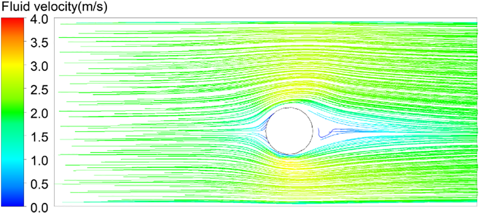
Figure 9: Velocity distribution in Group 1

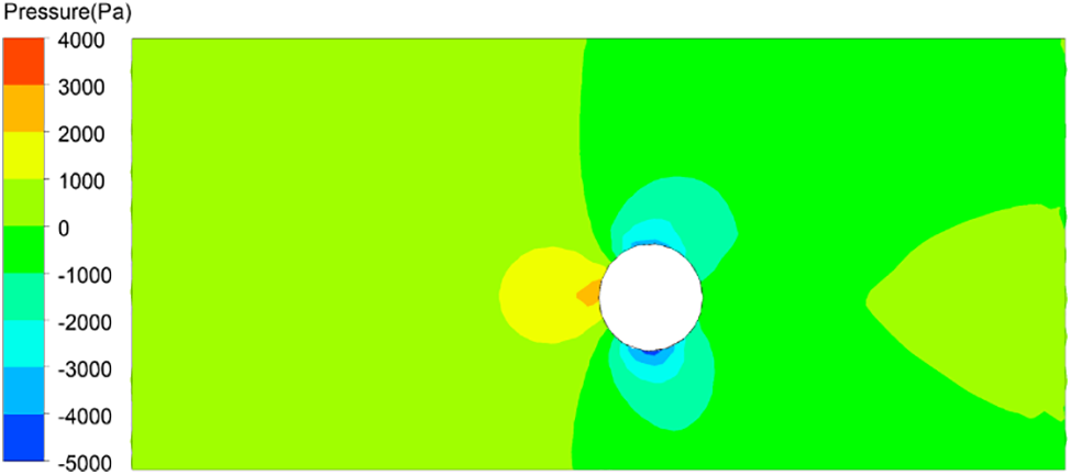
Figure 10: Pressure distribution in Group 1

The displacement of three points (marked A, B, and C) on the edge of the rag (Fig. 3) is shown in Fig. 11. The collision process can be divided into four consecutive stages [19].

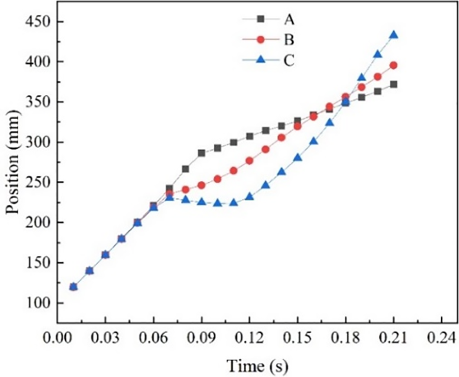
Figure 11: Evolution of three-point displacement in Group 1 with time

(1) In the first stage, the rag is displaced before colliding with the cylinder. The trajectory remains essentially linear from the release point.

(2) In the second stage, collision occurs. The middle point of the rag lags behind the stagnation point, while its tips continue translating along the flow direction as the rag wraps around the obstacle.

(3) In the third stage, the rag slides slowly on the upper part of the cylinder. The lower point (C) is pulled up while the other two points move slowly downstream.

(4) In the final stage, the rag is released behind the cylindrical obstacle.

The simulation results obtained in this study align with the four stages of rag movement summarized in the literature, validating the feasibility of the proposed method.

5.2 Effect of Speed on Trafficability

Table 3 shows three sets of experiments with the same angle and entry position, namely, Group 1 (2 m/s inlet velocity), Group 2 (1.5 m/s inlet velocity), and Group 3 (2.5 m/s inlet velocity), with the same angle and entry position, are shown in Fig. 12. The overall motion trends of the three experimental groups are similar, as are the relative changes in the displacement of the three points corresponding to each group. The motion process in Group 2 and Group 3 conforms to the four stages of rag collision mentioned above. However, speed has a marked effect on the rag’s movement. Although higher velocities result in faster overall movement and larger corresponding values, distinctions persist among the different groups. Prior to 0.18 s, the value of Point A in Group 1 exceeds that of Point C, signifying normal movement. However, after that time point, the value of Point A falls below that of Point C, indicating the flipping of the rag. Coincidentally, Group 3 undergoes a similar transition and the rag flips at 0.14 s, while no such phenomenon was observed in Group 2.

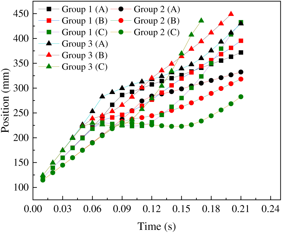
Figure 12: Evolution of three-point displacement with time in speed control group

Fig. 13 presents three corresponding streamline maps of fluid velocity, with similar overall distributions. The fluid velocity in the frontal and rear regions of the cylinder is low, whereas the fluid velocity in the upper and lower regions of the cylinder is relatively high. The maximum velocity roughly 1.5 times the inlet velocity, indicating a similar velocity variation. Furthermore, as speed increases, the vortices produced by the fluid behind the cylinder become more pronounced. Additionally, the maximum and minimum fluid velocity values intensify as the inlet velocity escalates.

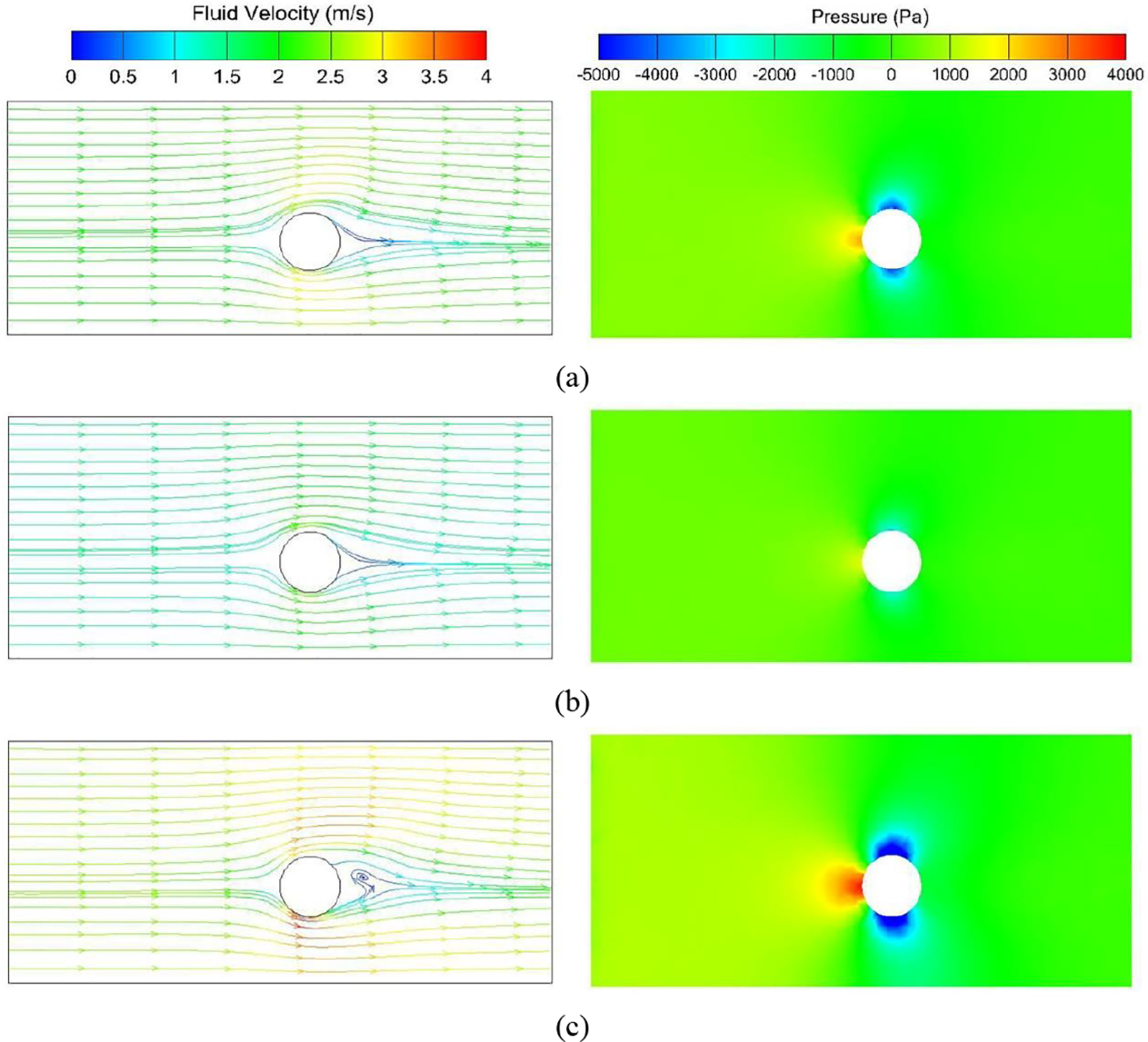
Figure 13: Velocity and pressure distribution at 0.09 s for (a) Group 1, (b) Group 2, (c) Group 3

Fig. 13 depicts the relationship between pressure distribution and velocity for three fluid sets. The various colors in the pressure contour map indicate that pressure fluctuations become more pronounced as the entry velocity rises. The fluid pressure on the left side of the cylinder increases, while the negative pressure in the upper and lower areas of the fluid diminishes. Simultaneously, the area of negative pressure expands, and the overall distribution remains analogous. As the speed increases, the maximum and minimum fluid pressure values also increase. Furthermore, due to the presence of the rag, the fluid pressure at the upper end of the cylinder surpasses the pressure at the lower end.

Fig. 14 shows the particle velocity distribution at 0.09 s. The position of the moving rag and the velocity of each area are relatively large at the upper end. In effect, higher speed is conducive to the rag’s passage through the cylinder.

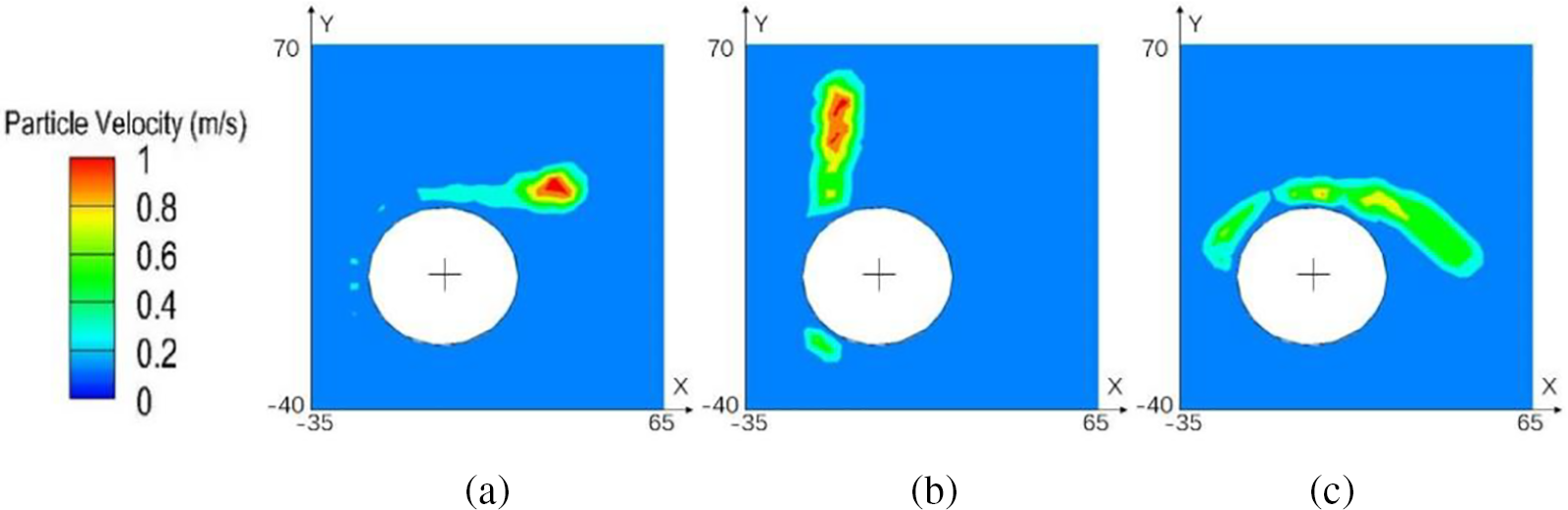
Figure 14: Relative position and velocity distribution at 0.09 s for (a) Group 1, (b) Group 2, (c) Group 3

5.3 Impact of Angle on Trafficability

Table 4 shows three sets of experiments with the same speed and entry position. The displacements of three points located on the edge of the rag in Groups 1, 2, and 3 at various time intervals are illustrated in Fig. 15. The entry inclinations for these three groups, relative to the horizontal direction, are 90°, 60°, and 45°, respectively. Three entry angles of the rag were examined (45°, 60°, and 90°) while keeping the entry speed and position constant. Examining Fig. 15 reveals a consistent overall motion trend among the three groups, with similar relative changes in the displacement of the three points corresponding to each group. Groups 4 and 5 also adhere to the four stages of the collision process mentioned above.

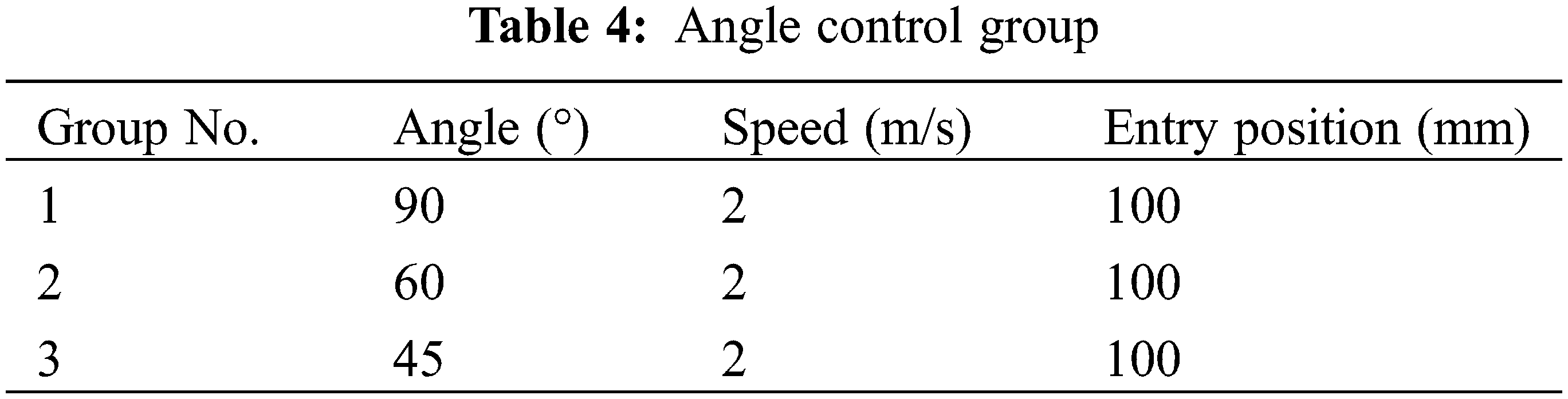
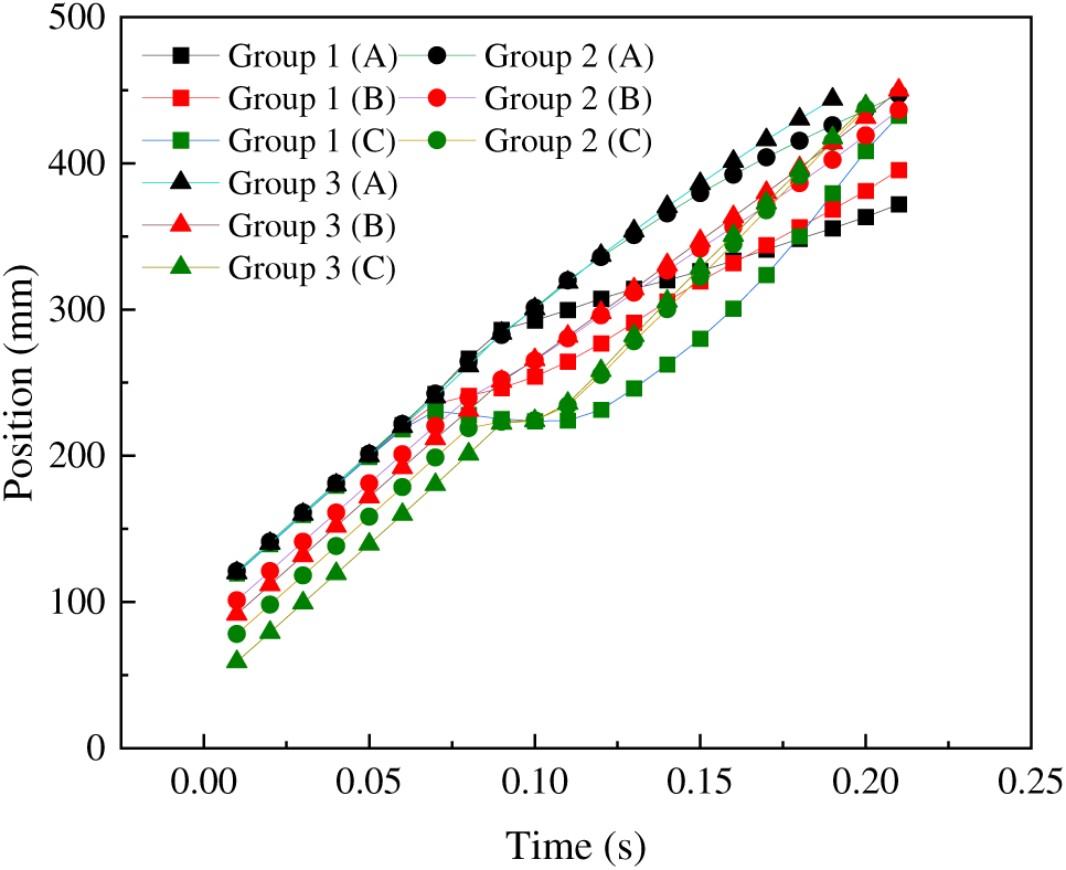
Figure 15: Evolution of three-point displacement with time in angle control group

Due to the angle inclination, the upper initial positions of the three groups are roughly at the same distance, while the middle and bottom positions of the 60° and 45° groups are farther behind. However, in the subsequent movement, the two groups increase steadily while the 90° group demonstrates a relatively flat area and a reversal. The last 45° group existed the tank promptly, but there is no substantial overall gap between the last three groups. The group that entered at 45° bends after passing through the cylinder. At 0.19 s, Point C at the bottom exceeds Point B at the middle, but when leaving the channel, the bottom (Point C) does not exceed the top (Point A). The 60° group also bends after passing through the cylinder. At 0.18 s, the bottom (Point C) exceeds the middle (Point B), and the bottom (Point C) surpasses the top (Point A) at 0.2 s. The 90° group completes a rag flip in 0.19 s, with the bottom (Point C) in the front and the top (Point A) at the back.

Fig. 16 shows velocity streamline diagrams of the three corresponding fluid groups, revealing a striking similarity in their overall distributions. The fluctuation of fluid velocity from the inlet to the left side of the cylinder is relatively small, approximately 2 m/s. As the fluid flows through the cylinder, its velocity decreases while increasing in the upper and lower regions. Notably, due to the smaller distance between the lower end of the cylinder and the channel boundary compared to the upper end, the fluid velocity on the lower side of the cylinder exceeds that on the upper side, leading to the formation of vortices of similar size on the right side of the cylinder. As these vortices gradually move away from the cylinder, velocity increases as both the maximum and minimum values exhibit similar distributions. This suggests that changing the angle does not significantly impact velocity, with the three groups experiencing similar changes. The overall magnitude and range of velocity changes are essentially identical, confirming the limited impact of angle on velocity.

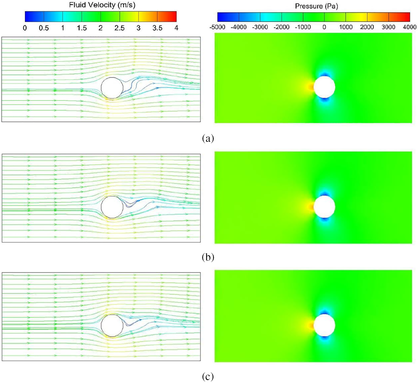
Figure 16: Velocity and pressure distribution at 0.15 s. (a) Group 1 (b) Group 2 (c) Group 3

The distributions of the three pressure groups are illustrated in Fig. 16. The pressure changes and distributions of the three groups appear to be roughly the same with varying angles. The pressure on the left side of the cylinder is higher than the pressure on the right side, and the pressure in the contact area between the fluid and the left side of the cylinder is the highest. Clear boundaries and similar positions are present in all three groups, with relatively low pressure in the upper and lower areas. Moreover, the maximum and minimum pressure values are similar across these groups. However, as the angle increases, the area where the fluid pressure on the lower side of the cylinder is less than −2000 Pa gradually expands.

From Fig. 17, it can be seen that these three groups exhibit similar positions at 0.15 s, with higher breaking speeds in the area near the upper boundary of the channel. The maximum velocity values are also comparable, all measuring 1 m/s. All three groups exhibit a trend of the rag bending. Based on these results, the incidence angle has a minimal impact on the rag’s trafficability. However, a 45° inclination is advantageous for the rag to pass through the cylinder.

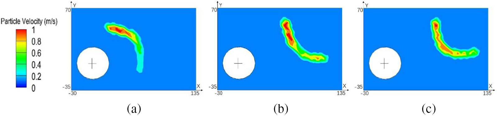
Figure 17: Relative position and velocity distribution at 0.15 s. (a) Group 1 (b) Group 2 (c) Group 3

5.4 Impact of Location on Trafficability

Table 5 shows three sets of experiments with the same angle and speed. Fig. 18 depicts the displacement over time for Groups 1, 2, and 3 at different entry positions. The velocities and entry angles of the three experiments are identical, with distances of 90, 100, and 110 mm from the entrance boundary of the channel, respectively. From Fig. 18, it is evident that the motion trends of the three groups of experiments are similar, and the relative displacement changes for the three points corresponding to each group are similar as well. The motion process of Groups 6 and 7 conforms to the four stages of the collision process described above.

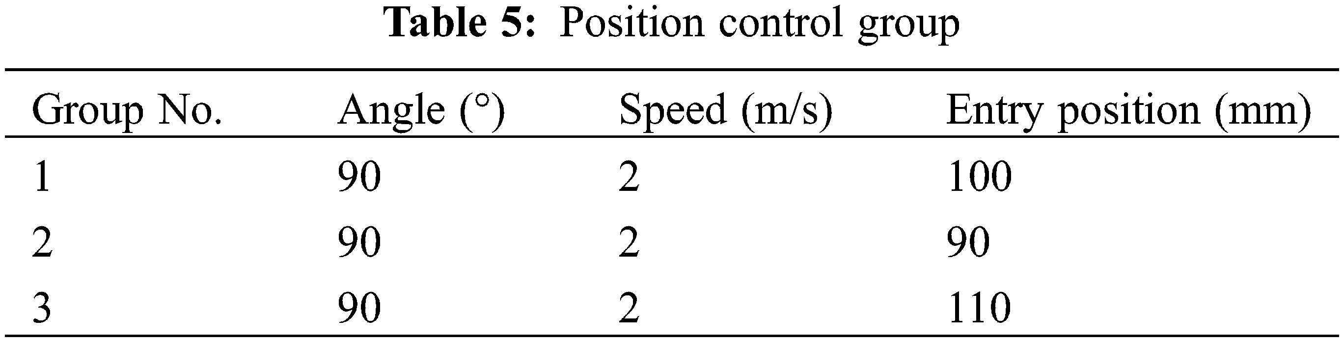
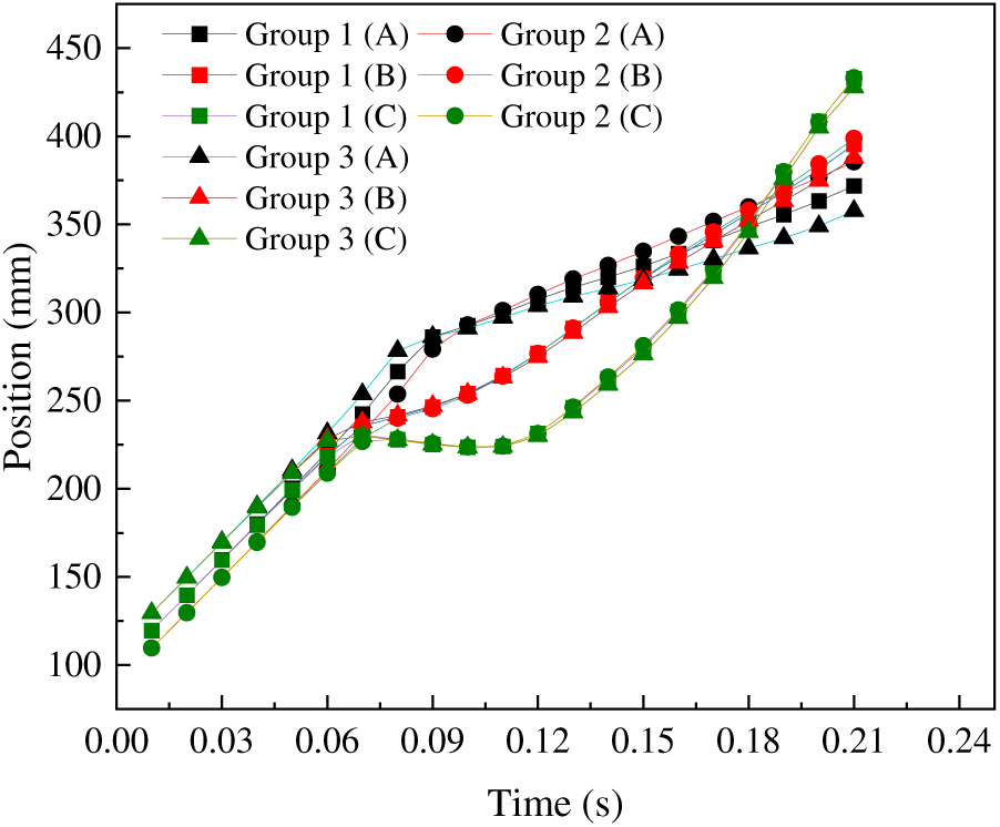
Figure 18: Evolution of three-point displacement with time in position control group

Prior to the collision with the cylinder at 0.08 s, the slopes of the three groups are essentially the same. The numerical differences at the corresponding points at the same time mirror those at the initial position. This indicates that the motions are comparable across the three groups of experiments. After 0.08 s, the positions of the three lower points (C) decrease, mainly due to rebounding of the lower area of the model after the collision, causing the position to move backward. After 0.12 s, the rag begins to leave the cylinder and resumes rightward movement, where the values began to increase. Subsequently, all three sets of rags begin to bend and fold after leaving the cylinder until flipping at 0.19 s. The displacement differences in the corresponding points are close to the initial differences for all three experimental groups.

The velocity streamlines of three sets of experiments with similar overall distributions are shown in Fig. 19. From the entrance to the left side of the cylinder, the fluid velocity fluctuates slightly at around 2 m/s. In the contact area between the fluid and the left side of the cylinder, the fluid velocity decreases while the velocity in the upper and lower areas increases. The maximum velocity of the three groups of experiments is also similar, measuring 3.5 m/s. As the fluid moves away from the cylinder, the velocity gradually decreases to 2 m/s, while the velocity distributions of the three groups are nearly identical. Therefore, changes in distance from the entrance boundary of the channel when the model enters have a negligible impact on speed. However, as the distance from the entrance boundary of the channel increases, the vortex on the right side of the cylinder gradually intensifies.

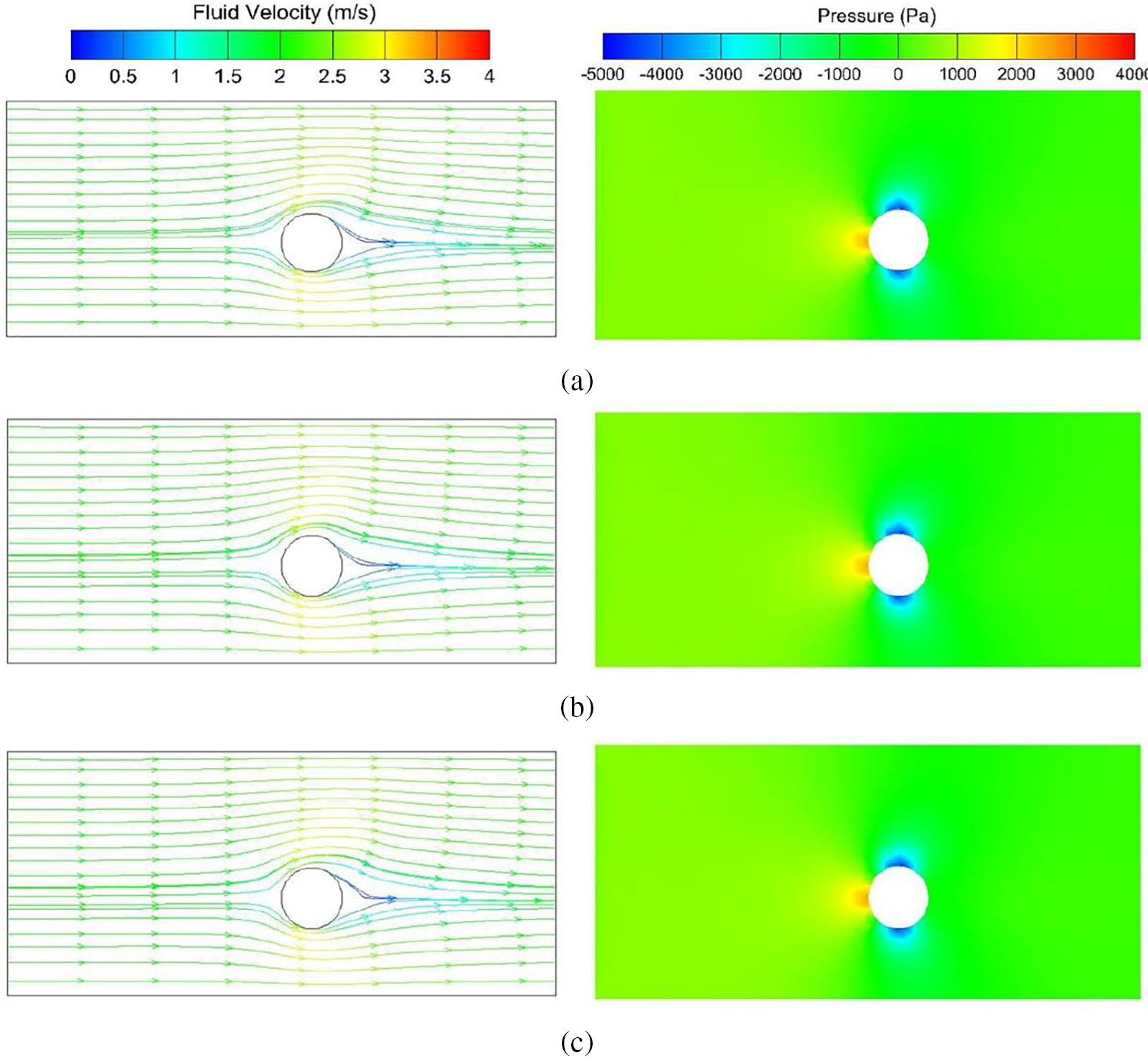
Figure 19: Velocity and pressure distribution at 0.09 s. (a) Group 1 (b) Group 2 (c) Group 3

Pressure cloud maps of three groups of experiments are also provided in Fig. 19, where the images reveal close similarities in the distributions of pressure among the three groups. Pressure is consistently higher on the left side of the cylinder and lower on the right side. The pressure in the upper and lower regions is also lower than the mid-section. The maximum and minimum pressure values are similar, and the pressure distributions are very close, indicating that changes in distance from the cylinder when the model enters have a negligible impact on pressure.

Fig. 20 displays a rag velocity cloud map as the rag moves in the channel at various entry distances for 0.09 s. The image reveals that the rag has a more forward-facing trajectory and higher top velocity when it enters the cylinder farther away from the inlet boundary.

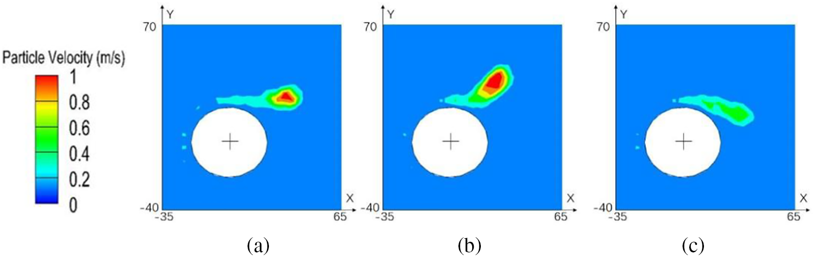
Figure 20: Relative position and velocity distribution at 0.09 s. (a) Group 1 (b) Group 2 (c) Group 3

6  Conclusion

A detailed study was conducted on the motion of rags in the flow around a cylinder. This study was conducted using the improved Hertz Mindlin (no slip) model to simulate the trafficability of rags at different inlet speeds, entry angles, and entry positions.

The main concluding observations are summarized as follows:

1.    Effect of inlet velocity on trafficability: Under identical conditions, an increase in inlet velocity results in higher velocities above and below the cylinder, accentuating the vortex on the right side of the cylinder. Additionally, the pressure difference on the left and upper sides of the cylinder increases with inlet velocity, facilitating easier passage of the rag through the cylinder. The passage time for square fibers is also shorter, with a maximum speed at 2.5 m/s which is 1 m/s higher than the maximum speed at 1.5 m/s.

2.    Impact of entry angle on trafficability: Under the same conditions, although the particle model inclined at 45° enters quickly, the final passage time does not differ compared to other angles, indicating a small impact on trafficability. This does have a slight impact on velocity, however, with a maximum velocity of approximately 3 m/s and a similar pressure distribution around the cylinder.

3.    Effect of entry position on trafficability: Under the same conditions, changes in the entry position have a minimal impact on speed and pressure during the rag’s passage. The overall distribution, maximum, and minimum values remain basically the same. Proximity to the cylinder facilitates easier passage.

Acknowledgement: The authors would like to thank the editor and the anonymous reviewers for their insightful comments and helpful suggestions to improve the quality of this manuscript, which significantly enhanced the paper’s presentation.

Funding Statement: This research was funded by the Zhejiang Provincial Natural Science Foundation of China (Grant Nos. LY21E060004, LGG22E060011), National Natural Science Foundation of China (Grant No. 51976193).

Author Contributions: The authors confirm contribution to the paper as follows: study conception and design: Yun Ren, Lianzheng Zhao; data collection: Lianzheng Zhao; analysis and interpretation of results: Xiaofan Mo, Shuihua Zheng, Youdong Yang; draft manuscript preparation: Yun Ren. All authors reviewed the results and approved the final version of the manuscript.

Availability of Data and Materials: The external characteristic data in this article was obtained through experiments, while the internal flow field data was obtained through specific software. Data will be made available on request.

Conflicts of Interest: The authors declare that they have no conflicts of interest to report regarding the present study.

References

1. Zobeyer H, Baki ABM, Nowrin SN. Interactions between tandem cylinders in an open channel: impact on mean and turbulent flow characteristics. Water. 2021;13(13):1718. [Google Scholar]

2. Kim J, Kim D. Flow-induced vibration and impact of a cylinder between two close sidewalls. J Fluid Mech. 2022;937:A28. [Google Scholar]

3. Vinodh A, Supradeepan K. A numerical study on influence of the control cylinder on two side-by-side cylinders. J Braz Soc Mech Sci. 2020;42(4):192. [Google Scholar]

4. Zhang T, Zhao YT. Analysis of flow field around a single cylinder at different reynolds numbers. New Technol New Process. 2020;389(5):33–6. [Google Scholar]

5. Zhao HX. Numerical simulation and mechanical analysis of flow around multiple cylinders. Res Explor Lab. 2023;42(7):130–5. [Google Scholar]

6. Afroz F, Sharif MAR. Numerical study of cross-flow around a circular cylinder with differently shaped span-wise surface grooves at low Reynolds number. Eur J Mech-B/Fluids. 2022;91:203–18. [Google Scholar]

7. Ali U, Islam M, Janajreh I. Hydrodynamic and thermal behavior of tandem, staggered, and side-by-side dual cylinders. Physics of Fluids. 2024;36(1):013605. [Google Scholar]

8. Alam MM, Rastan MR, Wang L, Zhou Y. Flows around two nonparallel tandem circular cylinders. J Wind Eng Ind Aerodyn. 2022;220:104870. [Google Scholar]

9. Rajpoot RS, Anirudh K, Dhinakaran S. Numerical investigation of unsteady flow across tandem square cylinders near a moving wall at Re = 100. Case Stud Therm Eng. 2021;26:101042. [Google Scholar]

10. Lee SJ, Lee SI, Park CW. Reducing the drag on a circular cylinder by upstream installation of a small control rod. Fluid Dyn Res. 2004;34(4):233. [Google Scholar]

11. Wang Y, Wang LG, Ji Y, Xi ZC, Zhang WW. A numerical study on the mechanisms producing forces on cylinders interacting with stratified shear environments. Fluid Dyn Mater Process. 2021;17:471–85. doi:https://doi.org/10.32604/fdmp.2021.014652. [Google Scholar] [CrossRef]

12. Huang YD, Wen WQ. Discrete eddy numerical study on particle diffusion distribution in the wake of liquid solid two phase circular cylinder flow. Appl Math Mech. 2006;27(4):477–83. [Google Scholar]

13. Huang YD, Wen WQ, Zhang HW. Numerical study on the effect of vortex on particle motion in unsteady unsteady liquid solid two phase flow. Adv Water Sci. 2002;13(1):1–8. [Google Scholar]

14. Li W, Liu M, Ji L, Li S, Song R, Wang C, et al. Study on the trajectory of tip leakage vortex and energy characteristics of mixed-flow pump under cavitation conditions. Ocean Eng. 2023;267:113225. [Google Scholar]

15. Li Y, Cao J, Xie C. Research on the wear characteristics of a bend pipe with a bump based on the coupled CFD-DEM. Multidiscip Digit Publish Inst. 2021;9(6):672. [Google Scholar]

16. Huang K. Performance research and optimization design of centrifugal pump based on CFD-DEM coupling calculation (Master Thesis). Jiangsu University: China; 2021. [Google Scholar]

17. Renzo AD, Maio F. Comparison of contact-force models for the simulation of collisions in DEM-based granular flow code. Chem Eng Sci. 2004;59(3):525–41. [Google Scholar]

18. RusSell R, Shirazi S, Macrae J. A new computational fluid dynamics model to predict flow profiles and erosion rates in dawnho1e completion equipment. In: SPE Annual Technical Conference and Exhibition; 2004. [Google Scholar]

19. Specklin M, Dubois P, Albadawi A, Delauré YMC. A fully immersed boundary solution coupled to a Lattice-Boltzmann solver for multiple fluid-structure interactions in turbulent rotating flows. J Fluids Struct. 2019;90:205–29. [Google Scholar]