A Numerical Investigation of the Effect of Boundary Conditions on Acoustic Pressure Distribution in a Sonochemical Reactor Chamber

1  Introduction

Acoustic cavitation occurs in a fluid under the influence of high-frequency sound waves (ultrasound). The cavitation phenomena involves sequential expansion, compression and destruction of gas bubbles [1,2]. Acoustic cavitation in fluid occurs at amplitude of acoustic pressure corresponding to cavitation threshold [3,4]. The results of acoustic cavitation investigations are used in the designing of chambers of sonochemical reactors and also make it possible to assess the contribution of cavitation effects to the processes of synthesis, extraction and separation of various substances [5–7].

One of the most important and time-consuming tasks in an experimental study of cavitation phenomena is the development and improvement of methods for visualizing acoustic fields in the cavitation zone. Observation and systematic study of cavitation zones often require high costs and special conditions to minimize the influence of measuring equipment and negative factors on fluid parameters.

One of the main methods of studying cavitation zones, which has become widespread, is considered a foil test method based on the erosion effect of aluminum foil [8,9]. It is cavitation erosion that occurs during the operation of various equipment that pushes many researchers to actively study cavitation in order to reduce noise, wear of the base material of the solid surface and reduce the risk of metal destruction [10,11]. A method based on the use of hydrophone has also become widespread. Due to the hydrophone capable of acting as a scanner, it is possible to obtain data, for example, on energy at various points of the acoustic field [12]. A significant limitation of the use of the hydrophone, in addition to its relatively high cost, is the effect of the sound receiver (microphone) on the acoustic field. As an alternative to the traditional hydrophone development of fiber-tip sensors, which have higher spatial resolution is conducted and allow to carry out measurements in limited spaces [13,14]. Despite this, the described methods are used both in the study of the evolution of cavitation zones and in the visualization of stationary acoustic fields in the cavitation zone.

It is known that the propagation of ultrasonic waves in the liquid significantly affects the distribution of pressure inside the sonochemical reactor. The distribution of acoustic pressure and the location of cavitation zones is determined by many factors: external conditions, the geometry of the sonochemical reactor chamber, the physicochemical properties of the fluid, the presence of various impurities and solid particles, as well as the configuration, location and frequency of the ultrasound source. The most effective method for studying the distribution of acoustic pressure under various conditions is numerical simulation [15–18]. Numerical simulation and experiments provide a more complete understanding of the acoustic field above the ultrasound source and a more detailed study of the pressure distribution in the cavitation zone [19–22].

In this work, the structure of the steady-state acoustic pressure field in the sonochemical reactor chamber is studied numerically. The influence of the piezoelectric transducer configuration and boundary conditions on the distribution of acoustic pressure in the fluid is studied. Comparison of the data on the location of cavitation zones obtained in the experiment by the foil test method and the structure of the simulated acoustic field in the fluid is carried out.

2  Methodology

The steady-state acoustic field is simulated using the Finite Element Method (FEM). The geometry of the sonochemical reactor chamber is shown schematically in Fig. 1. The dimensions of the camera are 160 × 110 × 116 mm3. The bottom and side surface of the chamber were assumed to be solid (Plexiglas-water boundary). The top of the chamber was assumed to be open (water-air boundary). A three-dimensional reactor chamber is considered to approach the conditions of the full-scale experiment [23].

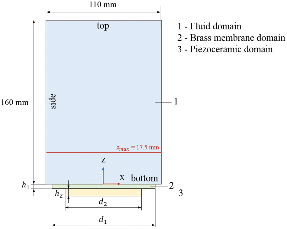
Figure 1: Geometry setup of the model. In the figure, zmax = 17.5 mm is the coordinate of the local maximum acoustic pressure pmax above the emitter

Sound waves in the fluid domain are generated by the surface of a thin brass membrane, which in turn oscillates under the action of a piezoelectric transducer (Fig. 1). This membrane with a diameter of d1 = 88 mm and a thickness of h1 = 0.4 mm contacts the bottom of the sonochemical reactor chamber. At the same time, the membrane contacts a piezoelectric transducer with a diameter of d2 = 62 mm located below. The thickness of the piezoelectric transducer h2 is 0.25; 0.40; 0.80; 1.0; 1.25; 2.5 and 5.0 mm.

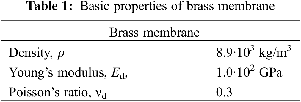
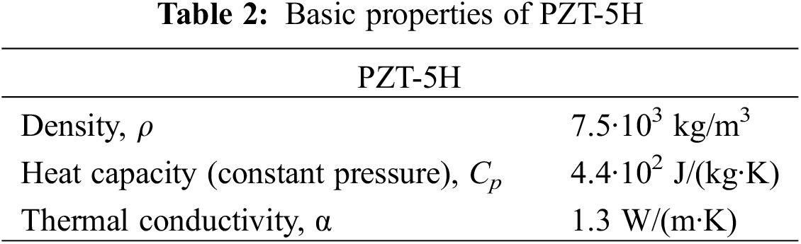
The piezoelectric transducer material is PZT-5H which is a type of lead zirconate titanate piezoceramics (PZT). The basic properties of brass and PZT-5H are shown in Tables 1 and 2.

The fluid domain is filled with water with parameters at a temperature of T0 = 293 K and a pressure of p0 = 105 Pa. The water density is ρ = 1.0·103 kg/m3, and the sound wave velocity is с = 1.5·103 m/s. Attenuation of sound waves in water is characterized by attenuation coefficient α = 1.3 Np/m. In this paper, the effect of convection and acoustic flow on the distribution of sound pressure in the liquid is not considered.

Simulation of the steady-state sound field in the water taking into account the interaction at the interfaces of the water, membrane and piezoelectric transducer. The calculation of stresses and deformations in the membrane is carried out together with the electric field in the piezoelectric transducer, which are also time-harmonic.

2.1 Acoustic Pressure Field (Fluid Domain)

The isentropic case is assumed, where the total change in entropy is zero and pressure is only a function of density. In addition, the case of an ideal fluid (water) is considered without taking into account the external mass force (gravity). Thus, taking into account the Fourier transform, the Helmoltz wave equation in the frequency domain is used in terms of the total acoustic pressure pt. The Helmholtz wave equation assumes a spatial constant sound velocity c0 and an average density of ρ [24].

∇⋅(−1ρ(∇pt))−ω2ρc2 pt=0 (1)

where ρ is the water density, c is the sound velocity in the water. It is assumed that the acoustic pressure in the water varies linearly with an angular frequency of ω = 2πf. The attenuation of the sound wave associated with the occurrence of cavitation gas bubbles and thermo-viscous processes in the water [25] is not taken into account in this work.

The interaction of a sound wave with a side boundary depends on whether the boundary is “sound hard” or “sound soft” free or closed. For an incident sound wave on a “sound hard” boundary, there is no normal velocity of water particles, i.e., n→⋅u→=0 . At the “sound soft” boundary, the sound pressure in the water is set equal to the initial pressure p0, or taken equal to p = 0. Therefore, different types of boundary conditions are modeled depending on the behavior of sound waves at the boundary (Table 3).

2.1.1 Type 1

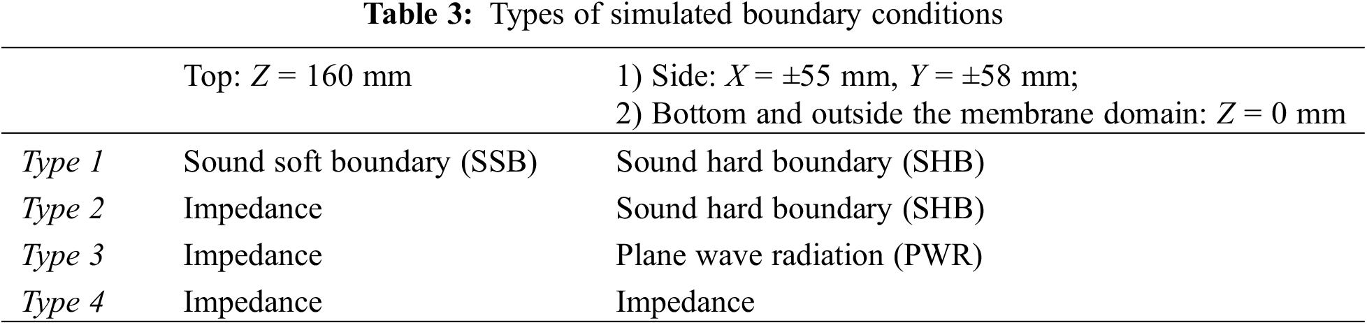
The top of the fluid domain (Z = 160 mm) is set to the Sound Soft Boundary (“SSB”) condition:

pt=0 (2)

This condition corresponds to a 180° phase shift of the sound wave at ideal reflection. In this case the acoustic impedance gets zero at the boundary.

At the side wall (X = ±55 mm, Y = ±58 mm) and bottom (Z = 0 (outside the membrane domain)) the Sound Hard Boundary (“SHB”) condition is set [24]:

∂pt∂n→=0 (3)

where n→ is the normal vector to the wall.

The reflection coefficient at the boundary is 1 (total reflection), which corresponds to the infinite impedance at the boundary. This condition also means that the normal derivative of the total acoustic pressure is 0 at the surface. Under this condition, the incident and reflected sound waves have the same phase [26].

2.1.2 Type 2

At the bottom (Z = 0 (outside the membrane domain)) and at the side wall (X = ±55 mm, Y = ±58 mm), the “SHB” condition is set. At the top (Z = 160 mm) the “Impedance” condition is set [27]:

1ρ∂pt∂n→=−iωptZ1 (4)

This condition implies that the top boundary is the water-air interface, which is characterized by the acoustic impedance Z1. The acoustic impedance denotes the ratio between the local pressure and the local normal particle velocity. The impedance boundary condition in this case is a good approximation of the locally reacting surface, for which the normal velocity at any point depends only on the pressure at this exact point. For example, an acoustic impedance of air is Z1 = 412 Pa·s/m (density 1.2 kg/m3, sound wave velocity 343 m/s).

2.1.3 Type 3

The top of the fluid domain (Z = 160 mm) is set to the “Impedance” condition. The side wall (X = ±55 mm, Y = ±58 mm) and bottom (Z = 0 (outside the membrane domain)) are assumed to be non-reflective, where the Plane Wave Radiation (“PWR”) condition is set [28]:

∂pt∂n→=−ikpt (5)

where k=ωc−iα –complex wave number with regard to attenuation, α–attenuation coefficient.

This condition corresponds to a non-reflective (absorbing) walls that allows the outgoing plane wave to leave the fluid domain with minimal reflections when the incident angle is close to normal.

2.1.4 Type 4

The top of the fluid domain (Z = 160 mm) is set to the “Impedance” condition (Eq. (4)).

The bottom (Z = 0 (outside the membrane domain)) and side wall (X = ±55 mm, Y = ±58 mm) of the chamber are characterized by acoustic impedance Z2 = 3.24·106 Pa·s/m (the density of plexiglass is 1.2·103 kg/m3, sound wave velocity 2.7·103 m/s [23,29]):

1ρ∂pt∂n→=−iωptZ2 (6)

2.2 Displacement, Stress and Deformation (Brass Membrane Domain)

Solid Mechanics module is used to simulate mechanical stresses and strain in a membrane (Fig. 1). The position of the solid particles is described by the Cauchy stress tensor σ in the approximation of an isotropic linear elastic medium:

ρ∂2u→∂t2=∇σ+fV→ (7)

where ρ is density of membrane material in undeformed state, u→ is vector of structural displacement, fV→ is vector of volumetric force acting on unit of deformed volume. Thermal losses in the membrane material during deformation are not taken into account.

At the side boundary of the membrane (X = ±d1/2), the condition u→ = 0 is set.

The relationship between the total acoustic pressure pt in the fluid domain (Pressure Acoustic module) with structural acceleration a→ in the membrane domain (Solid Mechanics module) is set using the Acoustic-Structure Boundary module. The interaction between the water and the membrane on the contact surface (Z = 0) is described by the following system of equations:

1ρ∂pt∂n→=−n→⋅a→ (8)

fA→=ptn→ (9)

where n→ is the normal vector to the contact surface, fA→ is the stress (force per unit area) experienced by the membrane from the water side.

2.3 Electric Field, Electric Displacement Field and Potential Distribution (Piezoceramic Domain)

To simulate the distribution of an electric field in a piezoelectric plate (Fig. 1a) the Electrostatics module is used. The relationship between the electric field and the electric potential φ is represented in the form of Gauss’s law:

∇⋅(ε0εrE→)=ρv (10)

E→=−∇φ (11)

where E→ is the electric field strength, ε0 is the electric constant, εr is the electric permeability of the brass, the ρ is the bulk density of the electric charge, and φ is the scalar electric potential.

At the side boundary of the piezoelectric transducer (X = ±d2/2) zero charge is set

n→⋅D→=0 (12)

At the bottom of the piezoelectric transducer (Z = −(h1 + h2)) the zero potential is set

φ=0 (13)

On the contact surface of the membrane and the piezoelectric transducer (Z = −h1), an AC electric potential is set φ = φ0, which is called the exciting voltage V0. This electric potential value, also called the excitation voltage V0, determines the amplitude of the sound wave to be excited. Excitation voltage is taken equal to V0 = 5.0 V.

2.4 Piezoelectric Effect (PZT-5H Domain)

The piezoelectric effect in the PZT-5H domain is considered in terms of linear piezoelectric material [30]:

T→=cES→−etE→ (14)

D→=eS→−εSE→ (15)

where T→ is the stress, S→ is the strain, E→ is the electric field at each point of the piezoelectric material, at each moment in time, and D→ is the charge density displacement vector. The superscript t denotes the transpose and cE is the stiffness or elasticity matrix, εS is the dielectric matrix and e the electromechanical coupling term.

The dynamics of the piezoelectric material are determined from Newton’s second law:

ρ∂2u→∂t2=∇⋅T→ (16)

In the absence of sources or sinks of charge

∇⋅D→=0 (17)

3  Mesh

Unstructured mesh with elements in the form of tetrahedra was used for numerical simulation. The parametric study of the mesh is based on the analysis of the convergence of the maximum acoustic pressure pmax at zmax = 17.5 mm above the brass membrane (Fig. 1) and the dependence of pmax on the mesh elements size Δ and the number of mesh elements N. The number of elements N was set manually for the fluid domain, brass membrane domain, and PZT-5H domain. Each domain was characterized by the number of elements m per height (thickness) of the domain. Mesh resolution increased near the edges of the membrane.

In the fluid domain (Fig. 1) the number of elements per height was set to m1 = 75. The maximum mesh element size Δmax is determined based on the number of mesh elements per wavelength λ:

Δmax = λ/n =c/(f⋅n) (18)

Based on the parametric study, the most optimal value n = 6 is determined which corresponds to Δ1max = 6.3 mm. The minimum mesh element size is Δ1min = 0.24 mm. The total number of mesh elements is N1 = 167700.

In the brass membrane domain (Fig. 1) the number of elements per height was set to m2 = 5. The maximum mesh element size is Δ2max = 3.23 mm. The minimum mesh element size is Δ2min = 0.032 mm. The total number of mesh elements is N2 = 7740.

In the PZT-5H domain (Fig. 1) the number of elements per height was set to m3 = 5. The maximum mesh element size is Δ3max = 3.23 mm. The minimum mesh element size is Δ3min = 0.032 mm. The total number of mesh elements is N3 = 4040.

User-controlled mesh was used to study the acoustic pressure distribution in the reactor chamber (Fig. 2).

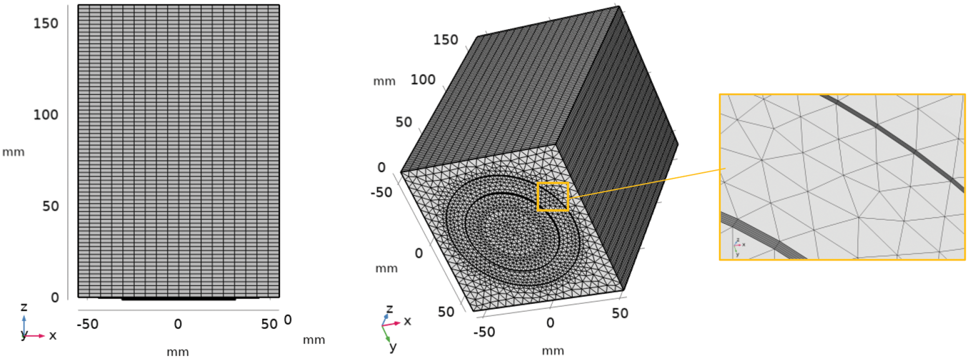
Figure 2: Unstructured tetrahedral user-controlled mesh

The mesh was also tested in the emitter region. The distribution of internal stresses during membrane deformation (brass membrane domain in Fig. 1) as well as the electrical potential within the piezoelectric transducer (PZT-5H domain in Fig. 1). The distribution of stresses and electrical potential for each domain was considered at Y = 0.

The distribution of stress tensor σ along Z = −h1/2 inside the membrane (Fig. 3a) and along Z = −(h1 + h2/2) inside the piezoelectric emitter (Fig. 3b) was obtained using a mesh at m = 5. The distribution of the electric potential inside the piezoelectric transducer is obtained at m = 5 (Fig. 4).

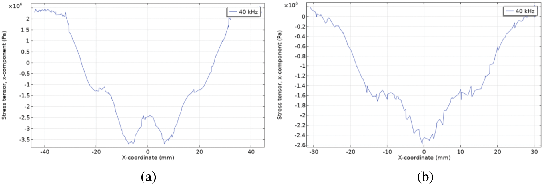
Figure 3: The distribution of internal stress σ along x-axis caused by: (a) membrane deformation; (b) piezoelectric transducer deformation

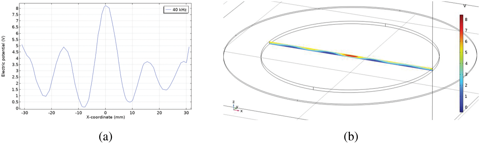
Figure 4: (a) The distribution electric potential φ along x-axis into piezoelectric transducer; (b) electric potential field inside a piezoelectric transducer

4  Results and Discussion

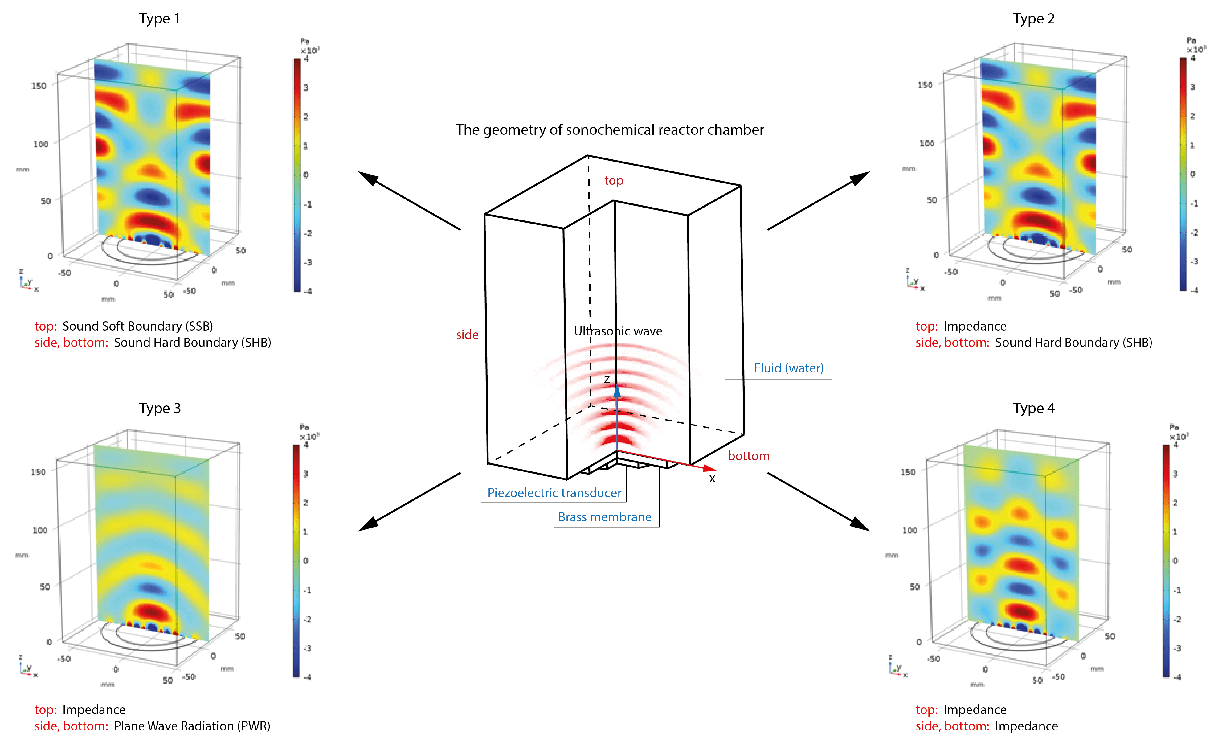
For acoustic standing waves the structure of the sound field depends on the geometry of reactor chamber and boundary conditions [26]. The use of different boundary conditions leads to a change in the location of the acoustic pressure peaks, which is due to the interaction of incident and reflected waves (interference).

The structure of the acoustic pressure field pt (x, z) above the emitter (brass membrane and piezoelectric transducer) has been studied numerically. Various boundary conditions are considered (Table 3). Fig. 5 shows the differences for distribution of total acoustic pressure in the reactor chamber created by a piezoelectric transducer with a thickness of h2 = 1.0 mm at f = 40 kHz. In each case, the acoustic pressure field is an alternation of high (red) and low (blue) pressure regions.

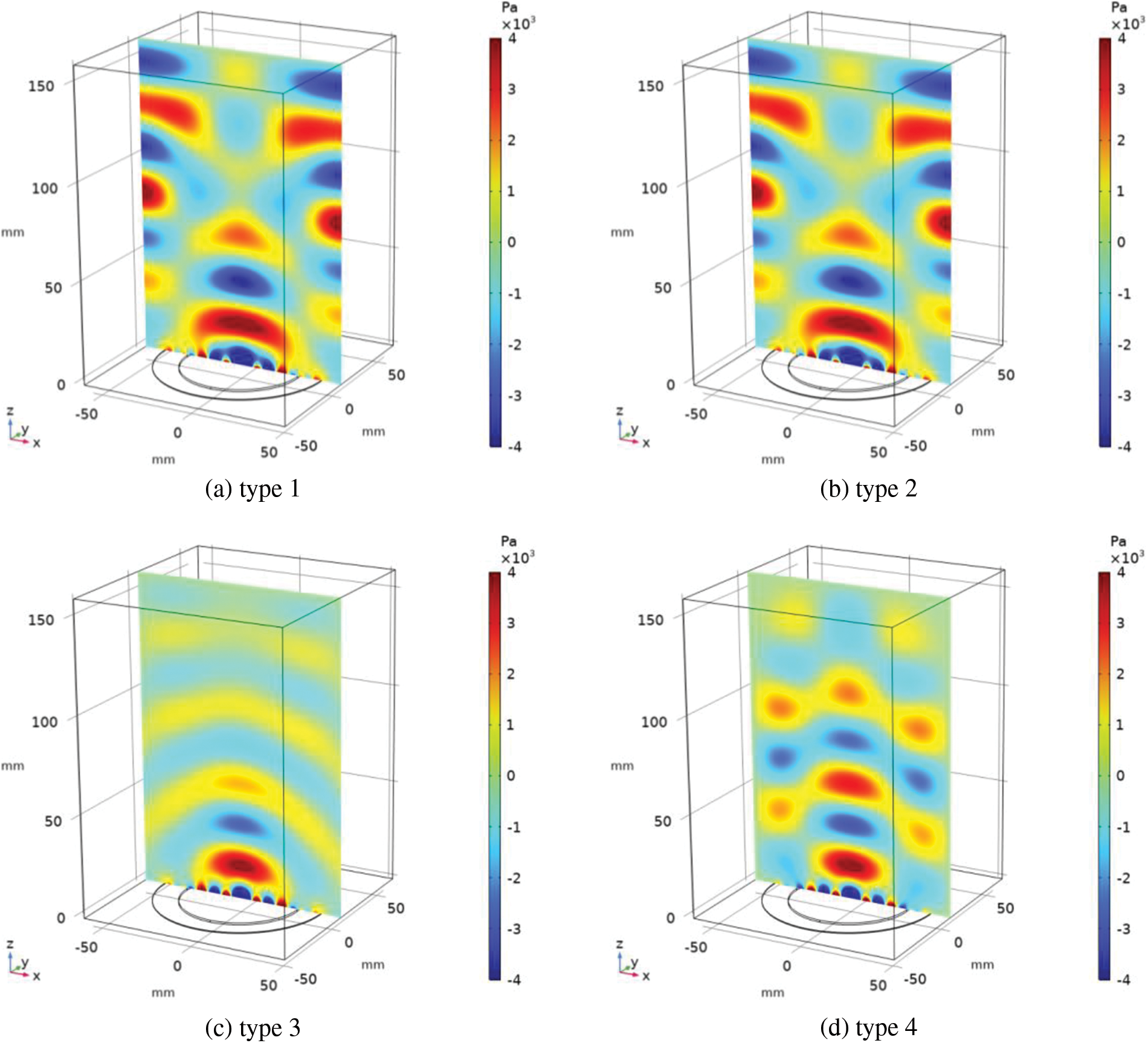
Figure 5: Acoustic pressure distribution in the center (Y = 0) of the chamber at the different types of boundary conditions (h2 = 1.0 mm, f = 40 kHz)

4.1 Effect of Boundary Conditions

For boundary conditions of type 1 and 2 (Figs. 5a,b) the zones of maximum total acoustic pressure (pt ~ 4·103 Pa) are mainly formed near the surface of the emitter and in the central part at the side walls. Additionally, on the acoustic axis of the emitter there are two local areas of high acoustic pressure: in the center of the reactor chamber pt ~ 2.5·103 Pa, at the top boundary pt ~ 1.2·103 Pa. The acoustic pressure distribution is the same for type 1 and 2 boundary conditions [31,32].

For non-reflective side walls (boundary conditions of type 3) the distribution of total acoustic pressure pt (x, z) in the reactor chamber is similar to the sound field from a point source in the area without boundaries (Fig. 5c). The maximum acoustic pressure region (pt ~ 4·103 Pa) in this case is also above the emitter surface. When moving away from the emitter, the ultrasonic wave attenuates and the wavefront bends. The amplitude of acoustic pressure pt ~ 1·103 Pa near the side boundaries of the reactor chamber. The sound wavefront tends to a plane wave shape near the top boundary of the reactor chamber. In the steady-state distribution of total acoustic pressure pt (x, z), there are four high-pressure and four low-pressure regions. Despite the most ordered structure of the sound field, this type of boundary conditions does not seem physical enough for the problem under consideration [21,26].

For boundary conditions of type 4 (Fig. 5d), in addition to the zone of maximum total acoustic pressure (pt ~ 4·103 Pa) near the emitter, there are several local areas of high pressure in the center of the chamber (along the acoustic axis of the emitter) and at the side walls of the chamber. Distribution of zones of highest and lowest pressure along acoustic axis of radiator is periodic and is caused by reflection from side boundaries. In addition, this type of boundary condition changes the pressure distribution near the top of chamber.

Boundary conditions of type 4 are further used to investigate the effect of emitter thickness on the distribution of total acoustic pressure pt (x, z) in the reactor chamber.

4.2 Effect of Piezoelectric Plate Thickness

For boundary conditions of type 4 dependence of the distribution of total acoustic pressure pt (x, z) on thickness h2 of piezoelectric transducer with frequency f = 40 kHz is considered.

When ultrasonic waves are excited in a water by an emitter of small thickness (h2 < 1 mm), a maximum acoustic pressure region is not formed above the emitter (Fig. 6a,b). The structure of acoustic pressure field is still an alternation of high and low pressure regions. In turn, a high pressure region (pt ~ 2·103 Pa) centered on the acoustic axis of the emitter is observed near the top boundary. In the center of the chamber there is a localized region of minimum total acoustic pressure (pt ~ (−2·103) Pa).

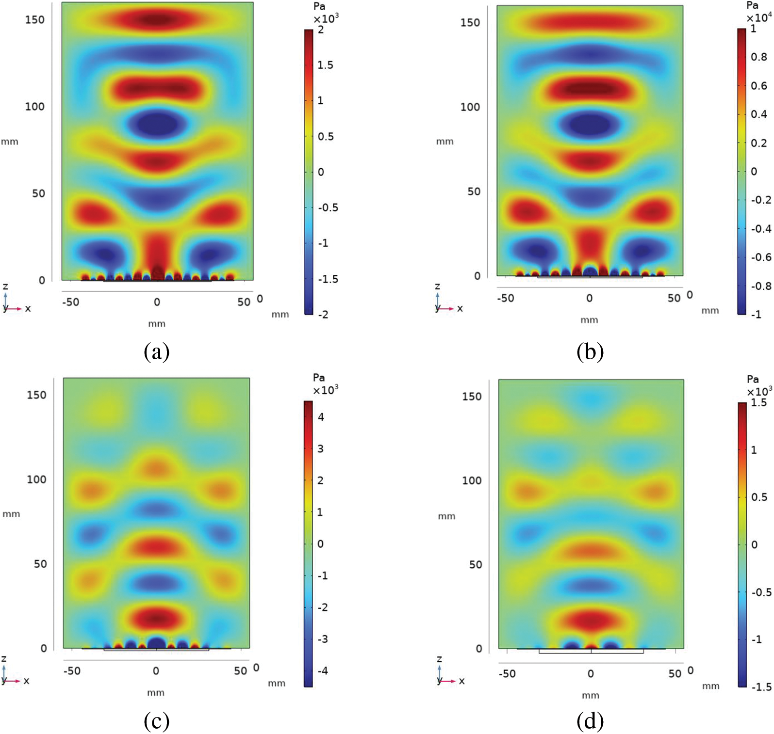
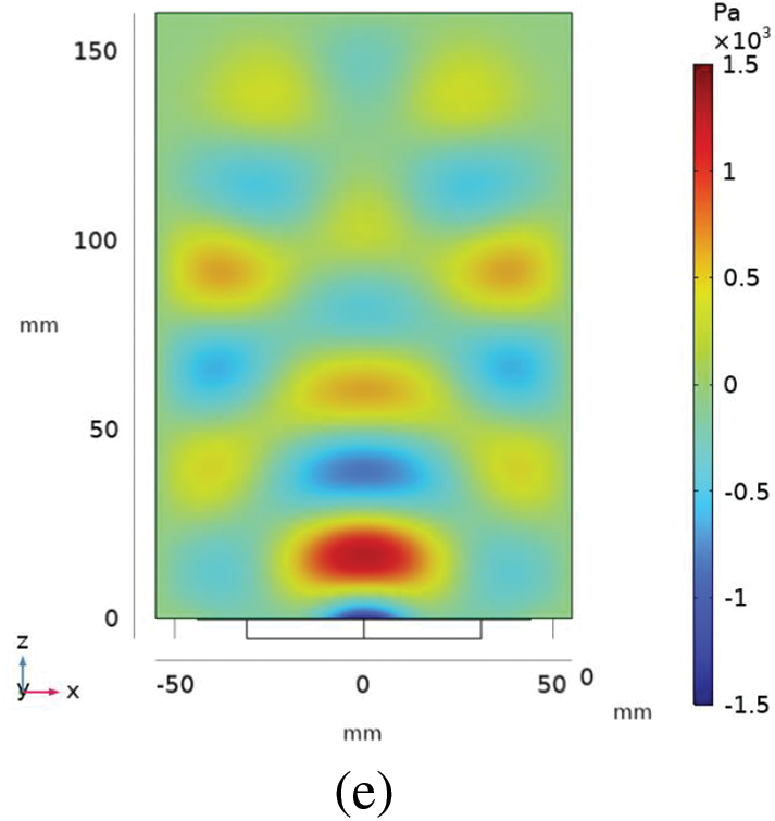
Figure 6: Effect of the thickness h2 of a piezoelectric plate with f = 40 kHz on the total acoustic pressure pt (x, z) in the center of the reactor chamber: (a) 0.4 mm; (b) 0.8 mm; (c) 1.0 mm; (d) 2.5 mm; (e) 5.0 mm

As the thickness of the emitter h2 increases, the acoustic pressure distribution changes (Fig. 6c–e). Region of maximum acoustic pressure above emitter is formed. Several high-pressure regions local to the side walls are formed in the water and alternate with the low-pressure regions. As the thickness h2 of the emitter increases, there is a change in distribution of total acoustic pressure pt (x, z) near the top boundary and a decrease in the pressure amplitude along the acoustic axis of the emitter.

The amplitude of the acoustic pressure at a distance of 17.5 mm from the emitter is maximum at h2 = 0.8 mm, which is apparently due to vibrations of the membrane in the resonance mode (Fig. 7). Therefore, a piezoelectric transducer at h2 = 0.8 mm and boundary conditions of type 4 is used to compare numerical simulation with experiment.

Figure 7: On axis total acoustic pressure pmax at 17.5 mm in front of the emitter

4.3 Comparison with Experiment

The results of numerical simulation are compared with the experiment data described in [23]. A parallelepiped-shaped cuvette with dimensions of 110 × 116 × 160 mm3 was used. The tank was made of acrylic glass with a thickness of 3 mm. As an ultrasound source, a piezoelectric transducer attached to a metal plate with a diameter of 88 mm was used, placed on the bottom of the tank so that the center of the emitter coincided with the center of the bottom. It was connected to an ultrasonic generator with a frequency of f = 40 kHz.

The distribution of cavitation zones was obtained from an experiment using the foil test method. The aluminum foil located in the center of the liquid layer is taken after 5 min from the start of the generator. The surface of the aluminum foil is destroyed by ultrasound as shown in Fig. 8a. The appearance of alternating horizontal black and white regions indicates the creation of a standing wave in the water. Localized erosion of aluminum foil is due to the distribution of energy in the standing wave between high pressure regions and low pressure regions. As a result, six cavitation zones (white regions) are formed in the water, distributed along the acoustic axis of the emitter. The average distance between the centers of the cavitation zones is 2.5 cm.

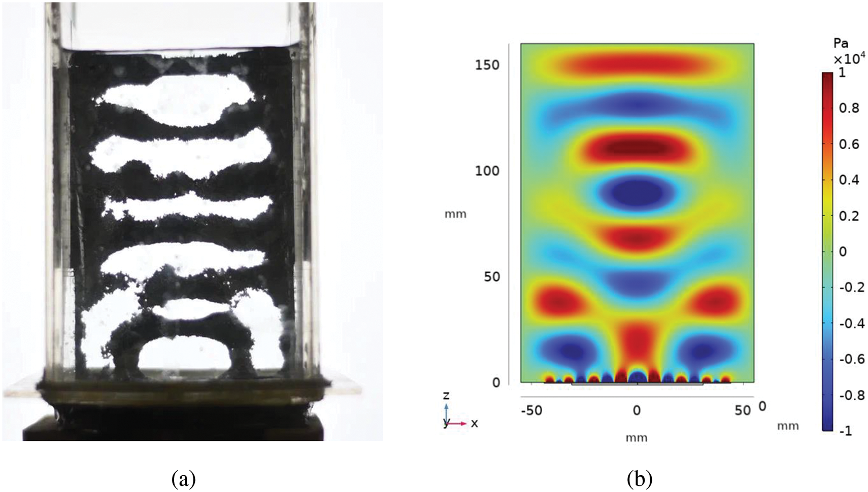
Figure 8: (a) The distribution of cavitation zones in the reactor chamber is studied using the foil test method (photo from article [22]. Copyright ©2020, IOP publishing); (b) total acoustic pressure pt (x, z) in the center of the reactor chamber (h2 = 0.8 mm, f = 40 kHz)

The intensity of cavitation activity is proportional to the size of the white regions on the foil (Fig. 8a). The intensity of erosion of the foil near the top of the tank is comparable in intensity to the cavitation activity near the emitter. Minimal cavitation activity appears near the side walls (black regions). Therefore, there is no destruction of the foil in this region.

The results of the numerical simulation were compared with experimental data to determine the type of boundary conditions that provide the best qualitative match of the acoustic pressure field structure in the central region of the reactor chamber [33]. The main assumption when comparing the sound field with the image of aluminum foil (Fig. 8a) consists in the fact that the location of cavitation zones in the water is associated with the structure of the steady sound field [21]. The comparison showed that the best agreement between the experiment data and the numerical results is achieved by boundary conditions of the type 4 with the thickness of the piezoelectric transducer h2 = 0.8 mm (Fig. 8b).

5  Conclusion

The acoustic pressure distribution in the sonochemical reactor chamber has been studied numerically. A study performed using COMSOL software showed the dependence of the sensitivity of the acoustic pressure field structure on boundary conditions for different thicknesses of the piezoelectric transducer. According to the results of the study, the amplitude of the acoustic pressure is minimal in the case of absorbing boundaries (type 3), and the attenuation becomes more significant as the thickness of the emitter increases.

The novelty of this study lies in the attempt to establish an interrelation between the location of the zones of maximum cavitation activity and the acoustic pressure field in the chamber of the sonochemical reactor. Comparison with experimental data by the foil test method showed that the regions of maximum sound pressure are located in the center of the reactor chamber along the acoustic axis of the emitter. For a more accurate comparison with the experiment, it seems more correct to use the impedance boundary condition (type 4). It is shown that the maximum amplitude of acoustic pressure in the water is achieved for a piezoelectric transducer with h2 = 0.8 mm at f = 40 kHz, which may indicate a resonant radiation mode.

The steady-state pressure field pt (x, z) obtained during numerical simulation is qualitatively consistent with the experimental data. The distribution of the sound field makes it possible to estimate the structure and location of the zones of cavitation activity in the reactor chamber.

Acknowledgement: None.

Funding Statement: The authors received no specific funding for this study.

Author Contributions: The authors confirm contribution to the paper as follows: study conception and design: Tatyana Lyubimova, Ivan Sboev, Konstantin Rybkin; data collection: Ivan Sboev, Michael Kuchinskiy, Konstantin Rybkin; analysis and interpretation of results: Ivan Sboev, Tatyana Lyubimova, Konstantin Rybkin, Michael Kuchinskiy; draft manuscript preparation: Ivan Sboev, Tatyana Lyubimova, Konstantin Rybkin. All authors reviewed the results and approved the final version of the manuscript.

Availability of Data and Materials: Data sets generated during the current study are available from the corresponding author on reasonable request.

Conflicts of Interest: The authors declare that they have no conflicts of interest to report regarding the present study.

References

1. Ashokkumar, M., Lee, J., Kentish, S., Grieser, F. (2007). Bubbles in an acoustic field: An overview. Ultrasonics Sonochemistry, 14(4), 470–475. [Google Scholar] [PubMed]

2. Ashokkumar, M. (2011). The characterization of acoustic cavitation bubbles—An overview. Ultrasonics Sonochemistry, 18(4), 864–872. [Google Scholar] [PubMed]

3. Yasui, K., Yasui, K. (2018). Acoustic cavitation and bubble dynamics, pp. 1–35. Cham: Springer International Publishing. [Google Scholar]

4. Nguyen, T. T., Asakura, Y., Koda, S., Yasuda, K. (2017). Dependence of cavitation, chemical effect, and mechanical effect thresholds on ultrasonic frequency. Ultrasonics Sonochemistry, 39, 301–306. [Google Scholar]

5. Leong, T., Johansson, L., Juliano, P., McArthur, S. L., Manasseh, R. (2013). Ultrasonic separation of particulate fluids in small and large scale systems: A review. Industrial & Engineering Chemistry Research, 52(47), 16555–16576. [Google Scholar]

6. Trujillo, F. J., Juliano, P., Barbosa-Cánovas, G., Knoerzer, K. (2014). Separation of suspensions and emulsions via ultrasonic standing waves—A review. Ultrasonics Sonochemistry, 21(6), 2151–2164. [Google Scholar] [PubMed]

7. Luo, X., Gong, H., Yin, H., He, Z., He, L. (2020). Optimization of acoustic parameters for ultrasonic separation of emulsions with different physical properties. Ultrasonics Sonochemistry, 68, 105221. https://doi.org/10.1016/j.ultsonch.2020.105221. [Google Scholar] [PubMed] [CrossRef]

8. Krefting, D., Mettin, R., Lauterborn, W. (2004). High-speed observation of acoustic cavitation erosion in multibubble systems. Ultrasonics Sonochemistry, 11(3–4), 119–123. https://doi.org/10.1016/j.ultsonch.2004.01.006. [Google Scholar] [PubMed] [CrossRef]

9. Dular, M., Osterman, A. (2008). Pit clustering in cavitation erosion. Wear, 265(5–6), 811–820. https://doi.org/10.1016/j.wear.2008.01.005 [Google Scholar] [CrossRef]

10. Liu, L., Yu, P. (2020). Design and experiment-based optimization of high-flow hydraulic one-way valves. Fluid Dynamics & Materials Processing, 16(2), 211–224. https://doi.org/10.32604/fdmp.2020.08168 [Google Scholar] [CrossRef]

11. Tong, D., Qin, S., Liu, Q., Li, Y., Lin, J. (2022). An analysis of the factors influencing cavitation in the cylinder liner of a diesel engine. Fluid Dynamics & Materials Processing, 18(6), 1667–1682. https://doi.org/10.32604/fdmp.2022.019768 [Google Scholar] [CrossRef]

12. Lafond, M., Asquier, N., Mestas, J. L. A., Carpentier, A., Umemura, S. I. et al. (2018). Evaluation of a three-hydrophone method for 2-D cavitation localization. IEEE Transactions on Ultrasonics, Ferroelectrics, and Frequency Control, 65(7), 1093–1101. https://doi.org/10.1109/TUFFC.2018.2825233 [Google Scholar] [CrossRef]

13. Koch, C., Jenderka, K. V. (2008). Measurement of sound field in cavitating media by an optical fibre-tip hydrophone. Ultrasonics Sonochemistry, 15(4), 502–509. https://doi.org/10.1016/j.ultsonch.2007.05.007. [Google Scholar] [PubMed] [CrossRef]

14. Arvengas, A., Davitt, K., Caupin, F. (2011). Fiber optic probe hydrophone for the study of acoustic cavitation in water. Review of Scientific Instruments, 82(3), 1000. https://doi.org/10.1063/1.3557420. [Google Scholar] [PubMed] [CrossRef]

15. Wei, Z., Weavers, L. K. (2016). Combining COMSOL modeling with acoustic pressure maps to design sono-reactors. Ultrasonics Sonochemistry, 31, 490–498. https://doi.org/10.1016/j.ultsonch.2016.01.036. [Google Scholar] [PubMed] [CrossRef]

16. Sutkar, V. S., Gogate, P. R., Csoka, L. (2010). Theoretical prediction of cavitational activity distribution in sonochemical reactors. Chemical Engineering Journal, 158(2), 290–295. https://doi.org/10.1016/j.cej.2010.01.049 [Google Scholar] [CrossRef]

17. Cao, P., Hao, C., Ma, C., Yang, H., Sun, R. (2021). Physical field simulation of the ultrasonic radiation method: An investigation of the vessel, probe position and power. Ultrasonics Sonochemistry, 76, 105626. [Google Scholar] [PubMed]

18. Hadi, N. A. H., Ahmad, A., Oladokun, O. (2019). Modelling pressure distribution in sonicated ethanol solution using COMSOL simulation. E3S Web of Conferences, 90, 02003. [Google Scholar]

19. Tao, T., Zhao, J., Wang, W. (2020). Study on the characterization method of ultrasonic cavitation field based on the numerical simulation of the amplitude of sound pressure. MATEC Web of Conferences, 319, 02003. [Google Scholar]

20. Servant, G., Laborde, J. L., Hita, A., Caltagirone, J. P., Gérard, A. (2001). Spatio-temporal dynamics of cavitation bubble clouds in a low frequency reactor: Comparison between theoretical and experimental results. Ultrasonics Sonochemistry, 8(3), 163–174. [Google Scholar] [PubMed]

21. Tudela, I., Sáez, V., Esclapez, M. D., Díez-García, M. I., Bonete, P. et al. (2014). Simulation of the spatial distribution of the acoustic pressure in sonochemical reactors with numerical methods: A review. Ultrasonics Sonochemistry, 21(3), 909–919. [Google Scholar] [PubMed]

22. Kuchinskiy, M. O., Lyubimova, T. P., Rybkin, K. A., Fattalov, O. O., Klimenko, L. S. et al. (2021). Experimental and numerical study of acoustic pressure distribution in a sonochemical reactor. Journal of Physics: Conference Series, 1809(1), 12025. https://doi.org/10.1088/1742-6596/1809/1/012025 [Google Scholar] [CrossRef]

23. Lyubimova, T., Rybkin, K., Fattalov, O., Kuchinskiy, M., Filippov, L. (2021). Experimental study of temporal dynamics of cavitation bubbles selectively attached to the solid surfaces of different hydrophobicity under the action of ultrasound. Ultrasonics, 117(5), 106516. https://doi.org/10.1016/j.ultras.2021.106516. [Google Scholar] [PubMed] [CrossRef]

24. Kaltenbacher, M. (2018). Computational acoustics. Cham: Springer International Publishing. [Google Scholar]

25. Bampouli, A., Goris, Q., van Olmen, J., Solmaz, S., Hussain, M. N. et al. (2023). Understanding the ultrasound field of high viscosity mixtures: Experimental and numerical investigation of a lab scale batch reactor. Ultrasonics Sonochemistry, 97(1–2), 106444. https://doi.org/10.1016/j.ultsonch.2023.106444. [Google Scholar] [PubMed] [CrossRef]

26. Rashwan, S. S., Mohany, A., Dincer, I. (2021). Development of efficient sonoreactor geometries for hydrogen production. International Journal of Hydrogen Energy, 46(29), 15219–15240. https://doi.org/10.1016/j.ijhydene.2021.02.113 [Google Scholar] [CrossRef]

27. Ajmal, M., Rusli, S., Fieg, G. (2016). Modeling and experimental validation of hydrodynamics in an ultrasonic batch reactor. Ultrasonics Sonochemistry, 28(7), 218–229. https://doi.org/10.1016/j.ultsonch.2015.07.015. [Google Scholar] [PubMed] [CrossRef]

28. Khan, M. U., Rehman, F., Saleem, M., Elahi, H., Sung, T. H. et al. (2023). Optimum driving of ultrasonic cleaner using impedance and FFT analysis with validation of image processing of perforated foils. Applied Sciences, 13(12), 6991. https://doi.org/10.3390/app13126991 [Google Scholar] [CrossRef]

29. Jiao, Q., Tan, X., Zhu, J. (2014). Numerical simulation of ultrasonic enhancement on mass transfer in liquid-solid reaction by a new computational model. Ultrasonics Sonochemistry, 21(2), 535–541. https://doi.org/10.1016/j.ultsonch.2013.09.002. [Google Scholar] [PubMed] [CrossRef]

30. Bolborici, V., Dawson, F. P., Pugh, M. C. (2010). Modeling of piezoelectric devices with the finite volume method. IEEE Transactions on Ultrasonics, Ferroelectrics, and Frequency Control, 57(7), 1673–1691. https://doi.org/10.1109/TUFFC.2010.1598. [Google Scholar] [PubMed] [CrossRef]

31. Yasui, K., Kozuka, T., Tuziuti, T., Towata, A., Iida, Y. et al. (2007). FEM calculation of an acoustic field in a sonochemical reactor. Ultrasonics Sonochemistry, 14(5), 605–614. https://doi.org/10.1016/j.ultsonch.2006.09.010. [Google Scholar] [PubMed] [CrossRef]

32. Sajjadi, B., Raman, A. A. A., Ibrahim, S. (2015). A comparative fluid flow characterisation in a low frequency/high power sonoreactor and mechanical stirred vessel. Ultrasonics Sonochemistry, 27, 359–373. https://doi.org/10.1016/j.ultsonch.2015.04.034. [Google Scholar] [PubMed] [CrossRef]

33. Wang, Y. C., Yao, M. C. (2013). Realization of cavitation fields based on the acoustic resonance modes in an immersion-type sonochemical reactor. Ultrasonics Sonochemistry, 20(1), 565–570. https://doi.org/10.1016/j.ultsonch.2012.07.026. [Google Scholar] [PubMed] [CrossRef]