A Novel Method for Determining the Void Fraction in Gas-Liquid Multi-Phase Systems Using a Dynamic Conductivity Probe

1  Introduction

Gas-liquid two-phase flow widely exists in the production and transportation of materials in the energy industry [1]. A gas-liquid two-phase flow system represents a stochastic, multivariable, nonlinear system. The complexity and randomness of the flow make it challenging to detect its parameters. With increasing requirements for accurate measurement, energy conservation, and control in industrial production, the need for precise measurement of two-phase flow parameters is becoming increasingly urgent. When characterizing parameters in gas-liquid two-phase flow, the phase fraction emerges as a crucial and illustrative parameter. It manifests in various forms, depending on the chosen units and definitions, namely the cross-sectional fraction, mass fraction, and volume fraction. The cross-sectional fraction, a component of phase fraction, is defined as the proportion of the area occupied by the flow of a specific phase at any given cross-sectional plane relative to the total cross-sectional area. Specifically, in gas-liquid two-phase flow, the phase fraction related to the gas component is conventionally referred to as the void fraction. The void fraction indicates the percentage of the gas phase in the cross-section of the pipe [2], reflecting the extent to which the gas phase dominates the cross-section during the passage of the two-phase mixture through any given cross-section. The void fraction is a key parameter of a two-phase flow, particularly for calculating the mixture density, mixture velocity, mixture viscosity, heat transfer coefficient, and pressure gradient of the flow [3]. It is noteworthy that the void fraction in quasi-homogeneous flow is usually higher than that in quasi-separated under similar gas and liquid flow rates [4]. The measurement of void fraction in gas-liquid two-phase flow has traditionally posed significant challenges in scientific research and practical applications. These challenges mainly arise from the complex and stochastic nature of gas-liquid flow patterns. Researchers have conducted numerous studies investigating how to identify flow patterns in gas-liquid two-phase flows using photon radiation [5]. For example, Abro et al. [6] proposed a multi-beam radiation technique, Faghihi et al. [7] developed a scheme that uses polyethylene phantoms to simulate two-phase flow, Nazemi et al. [8] introduced a broad beam gamma-ray transmission methodology, Khayat et al. [9] designed a multi-energy gamma-ray absorption measurement system, and Hanus et al. [10] proposed a gamma density method. The commonly used methods to measure void fraction include particle image velocimetry (PIV technique) [11,12], optical probe method [13], electrical method [14], tomography [15], and quick-break switch method [16]. However, the complexity of the flow process and the high measurement costs have limited the broad application of these new sensing technologies in two-phase flow parameter measurement.

The impedance method is a real-time technique with simple equipment requirements [17]. In 1967, Nassos et al. [18] utilized a conductance probe to measure the local void fraction of gas-liquid two-phase flow. In 2003, Lv et al. [19] conducted experimental research on void fraction measurement in gas-liquid two-phase flow using conductivity probes. The results demonstrated that the annular probe exhibited superior effectiveness compared to the parallel probe for void fraction measurement. Similarly, in the same year, Devia et al. [20] investigated two different electrode-structure sensor devices, namely flat electrodes and double annular electrodes, for void fraction measurement. By comparing the experimental results with theoretical predictions, they concluded that the double annular electrode structure yielded more accurate and stable measurements compared to flat electrodes. Furthermore, Fossa et al. [21], also in 2003, employed a circular probe to study horizontal intermittent flow in gas-liquid two-phase flow. They recorded various parameters along with the void fraction of the two-phase flow. In 2004, Sun et al. [22] chose to use a single ring electrode flush-mounted to the outer tube for excitation and utilized the inner conductive tube as the grounded electrode instead of using two distinct electrodes. In 2011, Ito et al. [23] developed a microwire mesh sensor (μWMS) based on interelectrode conductivity measurement for measuring gas-liquid two-phase flow in a narrow rectangular channel. In 2013, Ko et al. [24] used two annular electrodes to determine the liquid level of gas-liquid two-phase flow and numerically optimized the width and distance between the electrodes. In 2015, Ko et al. [25] employed a new conductivity probe consisting of two opposite electrodes and a small electrode installed in their gap to measure the gas volume fraction (GVF) in a horizontal channel. In 2017, Lee et al. [26] developed a new improved conductivity sensor capable of simultaneously measuring the area-averaged void fraction and structure velocity. In 2018, Xu et al. [27] aimed to enhance the measurement capability of capacitance sensors for void fraction in gas-liquid two-phase flow. They incorporated a rotating phase separation unit into the measurement unit of the capacitance sensor, effectively mitigating the influence of various gas-liquid two-phase flow patterns on void fraction measurement. Moreover, the traditional conductivity method relies on measuring the mixture’s conductivity and establishing a conductivity-water cut relationship model to calculate the water cut. However, this approach is sensitive to the salinity of the liquid phase and requires real-time calibration of the liquid phase’s salinity.

In this study, we utilized a cyclone device to induce forced annular flow in order to simplify the measurement of liquid phase distribution in gas-liquid two-phase flow, converting intricate and fluctuating flow patterns. This allowed for the achievement of a relatively uniform liquid film thickness, effectively eliminating the influence of flow patterns on void fraction measurement in two-phase flow. To overcome the limitations of conventional direct conductivity measurement devices, which only enable void fraction determination through static liquid film thickness measurement, we carefully designed a dynamic conductivity probe structure capable of reciprocating motion. Moreover, a measurement circuit system was implemented to facilitate remote and online assessment of the uniform liquid film, enabling real-time calculation of the gas-liquid void fraction.

2  Measurement Principle

Forced annular flow refers to the process of artificially manipulating the uncontrollable flow pattern into a gas-liquid two-phase ring flow using external forces, such as electromagnetic force, centrifugal force. In our study, we proposed a measurement device that incorporates a vane cyclone at the upstream section of the measuring tube and utilizes a reciprocating conductance probe. When the gas-liquid two-phase mixture passes through the cyclone, a strong swirling flow is generated due to centrifugal action. This causes the liquid in the mixture to be pushed towards the pipe wall, filming a high tangential velocity liquid film [28]. As a result, the liquid phase is uniformly distributed along the tube wall, while the gas phase is concentrated in the center, forming a gas core. This configuration creates a forced annular flow, which has a smoother and more distinct phase interface [29]. This characteristic allows for accurate measurement of various inherent flow parameters in gas-liquid two-phase flow and facilitates easier implementation.

Based on the work of Li et al. [30], this study presents a new dynamic conductivity sensor designed for real-time measurement of liquid flow. Instead of using a circumferential array conductivity probe, this novel reciprocating sensor employs conductance technique to measure the discrepancy in electrical conductivity between the phases of the mixture [31]. As shown in Fig. 1, when the metal tip of the conductivity sensor contacts the conductive liquid, and the voltage signal collector delivers a high voltage output. Conversely, when the metal tip encounters the gas phase, which has a much lower conductivity, the circuit experiences high resistance and the output voltage is low. The reciprocating motion depth of the sensor produces distinct voltage signal values, which are used for determination the liquid film thickness and subsequently calculating of the void fraction in the gas-liquid two-phase flow.

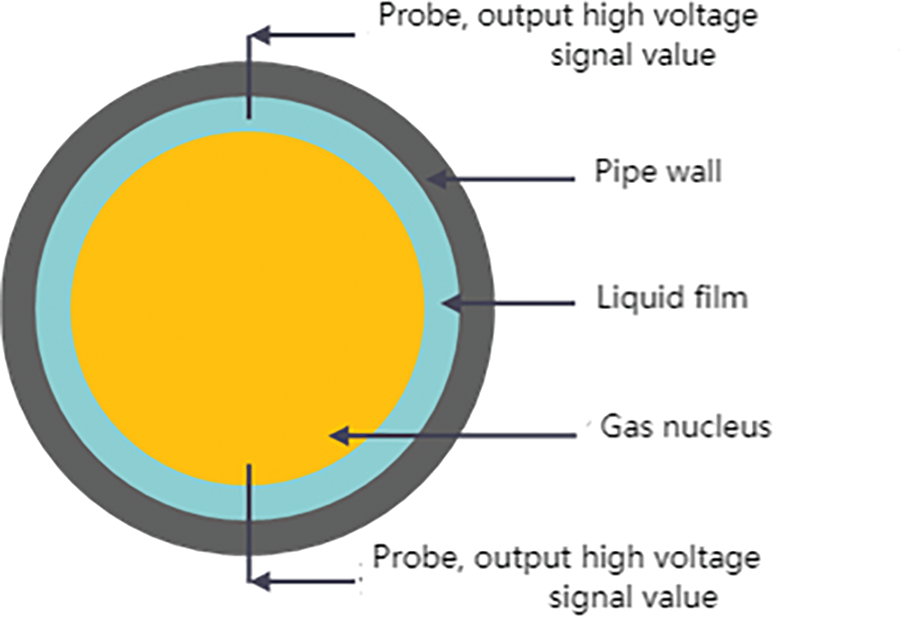
Figure 1: Schematic diagram of cavitation rate measurement by a forced annular current conductance method

The obtained measurement results were subjected to processing and analysis employing the duty cycle weighted average thickness algorithm [32]. Eq. (1) presents the mathematical expression utilized for calculating the average liquid film thickness during the statistical measurement period.

δavg=1T∫0Th(t)dt (1)

where, δavg is the average liquid film thickness (mm), T is the total sampling time in seconds (s), and h is the instantaneous value of the liquid film height (mm).

During the probe’s dynamic measurements, the signal waveform collected showed variations at different depths of insertion. Fig. 2 visually illustrates the waveform at different insertion depths, progressing from left to right, displaying high and low voltage waveforms. The solid line represents the average film thickness in the current state. When the probe tip made contact with the liquid film, the measurement circuit established conductivity, resulting in a high voltage signal equivalent to the power supply voltage. Throughout the designated measurement duration, the voltage output experienced cyclic changes in the form of a duty cycle, producing alternating high and low voltage levels.

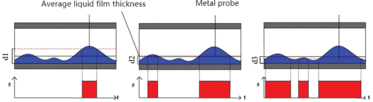
Figure 2: Illustration of measurements at different probe insertion depths

Measuring the film thickness of the same fluid wave at different depths proved challenging during the reciprocating motion of the conductivity probe due to the continuous forward movement of the fluid. However, this issue was addressed in this study by incorporating a cyclone device positioned at the leading end of the measurement section. This device effectively converted the complex flow pattern into a uniform “liquid film-gas core” annular flow. Furthermore, by utilizing an extended sampling time, the measurement signal values obtained at different depths of the probe could be considered representative of the average liquid film thickness at those specific depths.

The microscopic waveform analysis, depicted in Fig. 3, exhibits the horizontal axis representing collection time and the vertical axis representing the probe’s insertion depth, corresponding to the film thickness at that position. L1 represents the wavefront, L2 represents the minimum height of the gas-liquid interface during the experimental measurement period, and L3 represents the pipe wall. Assuming the total signal acquisition time is Tλ (s); h1 , h2 , h3 , h4 represent the distances from the probe tip to the pipe wall at different times (mm); and their corresponding conductive times are t1 , t2 , t3 , t4 (s).

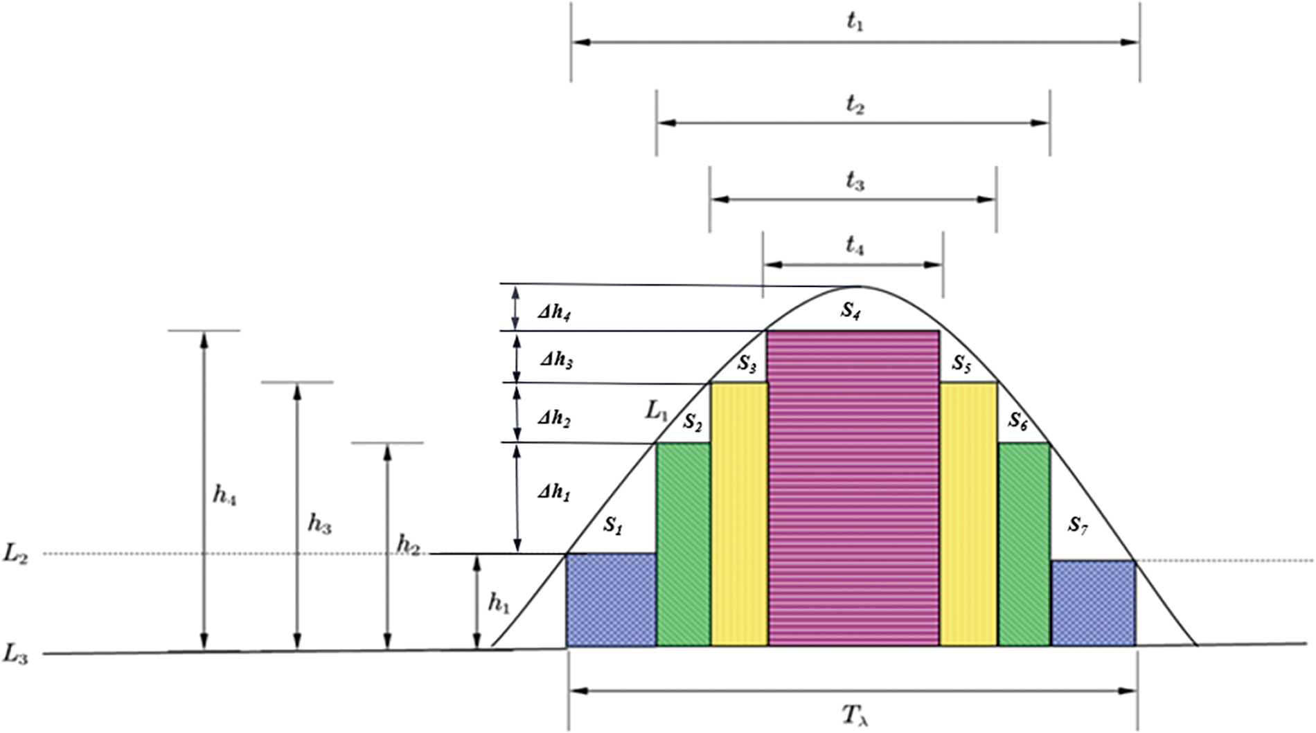
Figure 3: Principle of the weighted average thickness algorithm

Therefore, based on Eq. (2), the average liquid film thickness ( δavg ) could be calculated.

δavg=(h1×(t1−t2)+h2×(t2−t3)+h3×(t3−t4)+h4×t4)/Tλ (2)

where, t1/Tλ , t2/Tλ , t3/Tλ , t4/Tλ represent the void fractions ( Mi ) corresponding to different measurement heights. Assuming H is the initial height from the probe tip to the bottom of the pipe wall (mm), and Δhi is the increment of probe insertion depth (mm), the weighted average thickness algorithm could be derived as shown in Eq. (3). During the actual dynamic measurement process, different increments of probe insertion depth could be selected based on the required measurement accuracy.

δavg= M⋅H+(H−Δh1)(M2−M1)+(H−Δh1−Δh2)(M3−M2)+⋯+(H−Δh1−Δh2−⋯⋯Δhi)(Mi+1−Mi) (3)

The main error of this method occurs when calculating the area formed by the waveform and the wall surface of the pipe using the duty cycle and the height from the probe tip to the bottom of the pipe. It is evident from Eq. (3) that Si(i=1,2,...,7) was not calculated in the formula for obtaining the average liquid film thickness is the fundamental source of the error. Si(i=1,2,...,7) could be approximately considered as a triangle, and the relative error could be calculated by Eq. (4).

ei=Δhi2δavg (4)

With the average liquid film thickness, the void fraction could be calculated using Eq. (5).

ε=(R0−δavg)2R02 (5)

where, R0 represents the radius of the pipe.

3  Measuring System

3.1 Conductance Probe

The study employed a single-tip conductivity probe, consisting of a conductive metal needle, an insulating layer, a conductive metal tube, and a conductive wire. The needle was a 0.3 mm diameter acupuncture needle, the insulating layer was a 0.4 mm diameter polytetrafluoroethylene capillary, and the metal tube was a stainless-steel capillary with an inner diameter of 0.5 mm and a wall thickness of 0.25 mm. During the fabrication of the probe, the needle was first inserted into the insulating layer, and then both were inserted into the conductive metal tube. The gap between the needle and the insulating layer, as well as the outer side of the insulating layer, was filled with PVC insulation adhesive to ensure complete insulation between the needle and the stainless-steel capillary, and to maintain the overall stability and tightness of the probe. The schematic diagram of the probe composition is shown in Fig. 4.

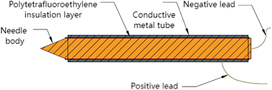
Figure 4: Component diagram of conductive probe

In addition, in considering of the reciprocal movement of the proposed conductivity probe measurement structure in this study, a reciprocal sealing mechanism was implemented. This mechanism utilized Y-shaped chloroprene rubber sealing rings and O-ring nitrile rubber seals to establish a reliable seal between the probe structure and the inner wall of the metal cylinder. The probe structure, which includes these sealing components, is depicted in Fig. 5.

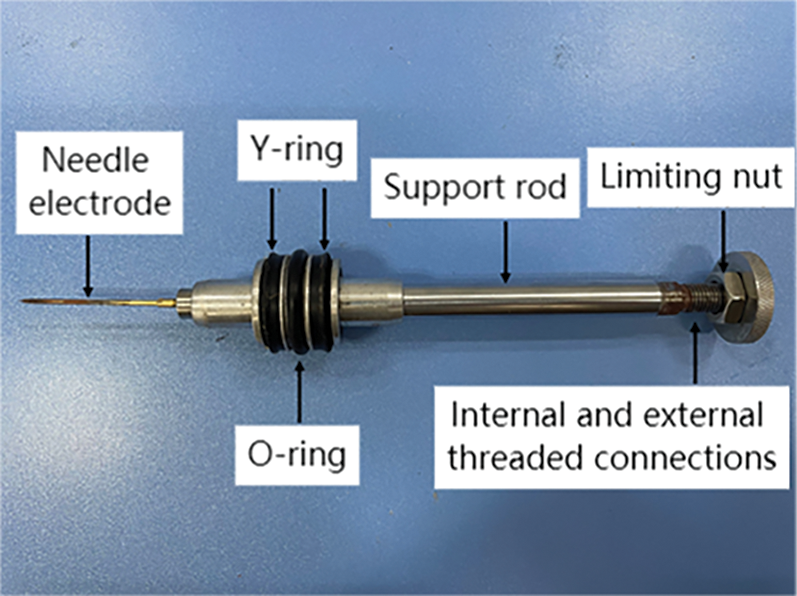
Figure 5: Physical structure of the conductive probe

3.2 Probe Automatic Reciprocating Movement Device

To facilitate the reciprocating motion of the probe during dynamic experimental measurements, a meticulously developed probe automatic advancement device was utilized. This device consisted of a probe automatic propulsion device and a remote controller.

The probe automatic propulsion device was primarily composed of a frame and a motor. The remote controller had eight functional buttons, enabling the adjustment of parameters such as speed, operating time, and operating mode of the conductivity probe. At the control panel’s periphery, multiple interfaces were integrated, encompassing limit switches, a USB data transmission interface, and a communication interface. These interfaces established direct communication with a computer, facilitating the recording and storage of the probe’s forward distance (depth inserted into the pipeline) and duration while being operated with the probe automatic propulsion device. Fig. 6 shows a visual representation.

Figure 6: Reciprocating movement measurement device

3.3 Signal Acquisition and Processing System

In this investigation, the conductivity method was used for liquid holdup measurement, focusing exclusively on the circuit’s conductivity and disregarding measurement errors caused by metal polarization. Therefore, a DC stabilized power supply was utilized to provide the necessary electrical energy, ensuring energy efficiency and environmental sustainability. The measurement circuit consisted of a probe measurement unit, power supply follower, data acquisition device, and computer. Within the measurement circuit, the conductivity probe acted as the negative terminal, while the steel pipe segment functioned as the positive terminal. During the measurement process, when the probe engaged in measurements, it formed a closed loop connection with the steel pipe segment. As the probe steadily progressed forward, it generated a high voltage signal upon contact with the liquid phase and a low voltage signal when in contact with the gas core, repeating this cyclic process. The measurement circuit configuration is illustrated in Fig. 7.

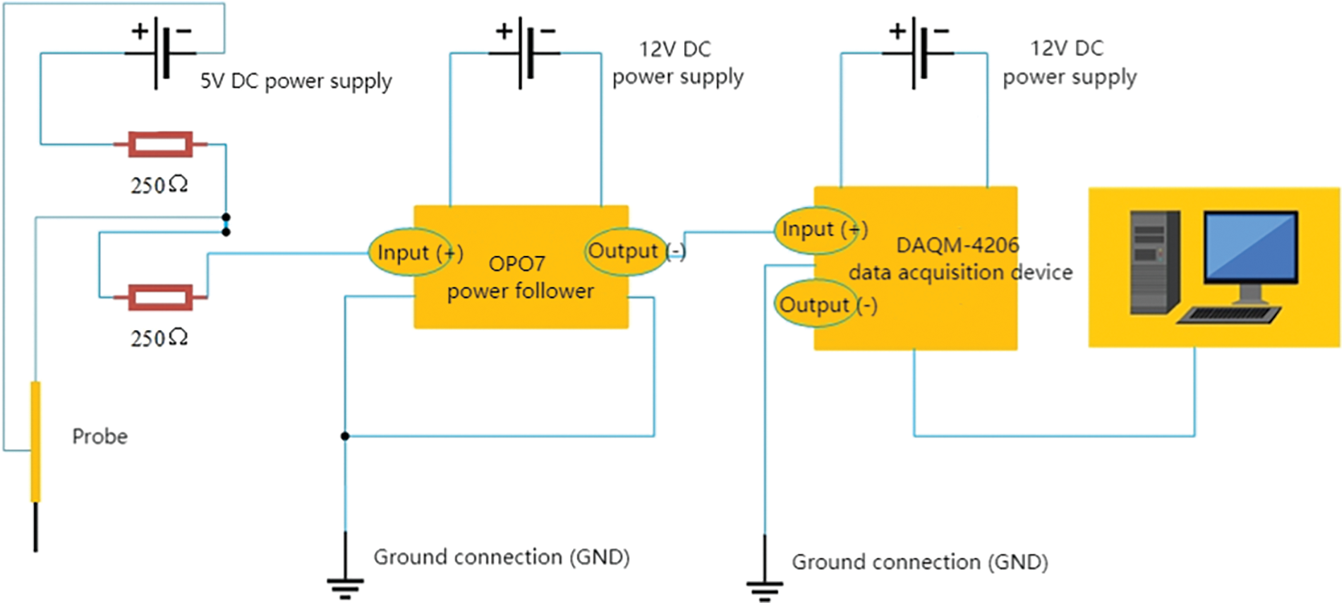
Figure 7: Conductivity measurement circuit

4  Experimental System and Measurement Method

4.1 Experimental System

This experiment was conducted at the Multiphase Flow Laboratory of the Yangtze University-Sinopec Gas Lift Experiment Base, kowned for its expertise in multiphase flow research. The experimental setup, as shown in Fig. 8, depicted the flowchart of the experimental configuration.

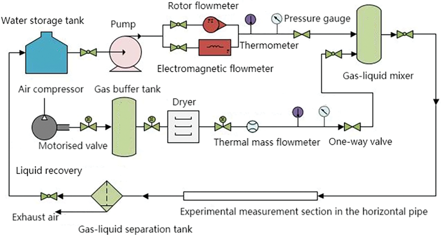
Figure 8: Flowchart of the experimental setup for measuring liquid film thickness

Air and water were chosen as the experimental media to simulate gas-liquid two-phase flow conditions. During the experiment, the gas was directed to the gas buffer tank after undergoing compression with an air compressor. It then passed through a dryer to ensure its quality and entered the gas-liquid mixer. On the other hand, the liquid phase was pumped from the water storage tank into the gas-liquid mixer utilizing a dedicated pump. Real-time data acquisition of physical parameters for both the gas and liquid phases was facilitated through the installation of flow meters, thermometers, and pressure gauges along the gas and liquid branches. To prevent backflow caused by excessive gas flow rate, one-way valves were strategically placed in both branches. Once thorough mixing occurred, the gas-liquid two-phase mixture was directed to the horizontal measurement pipe for the measurement of the liquid film thickness. Following this, the mixture underwent phase separation within the gas-liquid separation tank. The separated liquid phase was then returned to the water storage tank for recycling, while the gas phase was discharged into the atmosphere directly, ensuring safe and environmentally friendly operation.

The flow rates of the gas and liquid phases were precisely controlled using LabVIEW software, ensuring accurate and reliable measurements. The gas phase was pressurized utilizing a single-screw air compressor, providing a wide flow rate range from 0 to 2300 m3/h. To accurately measure the flow rate of the gas phase, a thermal mass flow meter was employed, with a measurement range of 5 to 400 m3/h and an accuracy of ±1.5%. On the other hand, the liquid phase was pressurized using a multistage centrifugal pump, offering a flow rate range from 0 to 6.3 m3/h. To determine the flow rate of the liquid phase, both a rotor flow meter and an electromagnetic flow meter were utilized. The rotor flow meter covered a measurement range of 0 to 0.4 m3/h, with a measurement accuracy of ±1.5%. Meanwhile, the electromagnetic flow meter had a measurement range of 0.3 to 3 m3/h, with a measurement accuracy of ±0.5%.

Once the gas and liquid phases were fully mixed, the resulting gas-liquid two-phase mixture entered the horizontal measurement pipe section. Within this section, it passed through a vane-type swirl generator, which facilitated the formation of a stable annular flow of a specific length. Subsequently, the mixture passed through a reciprocating dynamic conductivity sensor, and the corresponding voltage signals were captured and processed using a data acquisition system. The recording duration for each measurement was set at 1 min to capture sufficient data. A visual representation of the experimental setup in the measurement pipe section is shown in Fig. 9.

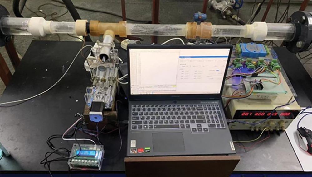
Figure 9: Online measurement experimental setup of the reciprocating dynamic conductivity sensor

The experimental setup focused on a horizontally positioned gas-liquid pipeline, which included the installation of a vane-type swirl generator upstream of the measurement pipe section. This setup effectively transformed the complex and diverse flow patterns into a forced annular flow. The pipeline had an inner diameter of 40 mm, and the experiment was conducted under normal temperature and pressure conditions (25°C, 101 kPa). During the experiment, the gas phase superficial velocity ranged from 5 to 20 m/s, corresponding to a flow rate range of 22.6 to 90.5 m3/h. Similarly, the liquid phase superficial velocity spanned from 0.088 to 0.48 m/s, corresponding to a flow rate range of 0.4 to 2.2 m3/h. The experimental scheme could be divided into two situations: one where the liquid phase volume fraction α (%) ranged from 1% to 12% while the gas phase superficial velocity vsg remained unchanged at 5 m/s; the other where the gas phase superficial velocity vsg (m/s) ranged from 5 to 12 m/s while the liquid phase volume fraction α remained unchanged at 8%. To ensure reliable signal acquisition and prevent leakage during the experiment, a seal check of the entire experimental system was conducted prior to performing the measurement experiment with the reciprocating dynamic conductivity sensor. The signal acquisition circuit was excited by a 5V DC voltage, establishing the necessary electrical environment for accurate data collection.

4.2 Experimental Process

The procedure for measuring the dynamic void fraction is illustrated in Fig. 10. In this procedure, a threshold value (R) of 90% was set for the void fraction. When the liquid phase holdup of the inner wall of the measuring tube exceeded 90%, it indicated the formation of a liquid annulus [33]. First, the remote controller was used to adjust the insertion depth of the probe. The distance H and duty cycle Mi between the tip of the probe and the measuring tube section were recorded when the output value of the voltage acquisition module was high. Then, the controller was further adjusted to continue moving the conductance probe forward Δh , and the Mi value was compared with the threshold value R. The average thickness of the dynamic liquid film at the measuring point was calculated.

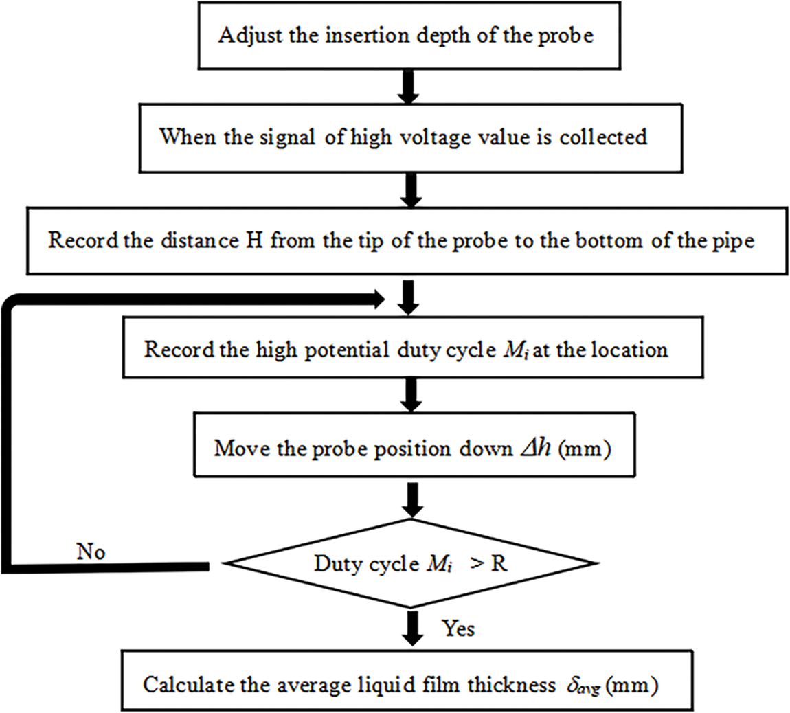
Figure 10: Flowchart for measuring average liquid film thickness

5  Experimental Results and Analysis

5.1 Analysis of Duty Cycle Calculation Results

The voltage and time data obtained from the acquisition module underwent processing to determine the duty cycle within a specific time interval. For instance, let us consider a scenario where the gas phase superficial velocity was 5 m/s and the liquid phase volume fraction was 8%. During the dynamic experiment, noticeable fluctuations were observed in the voltage signal output as the distance between the probe tip of the conductivity sensor and the bottom of the pipe changed. To ensure sufficirnt signal acquisition time, data within a 60-s interval were extracted to calculate the duty cycle, as shown in Fig. 11.

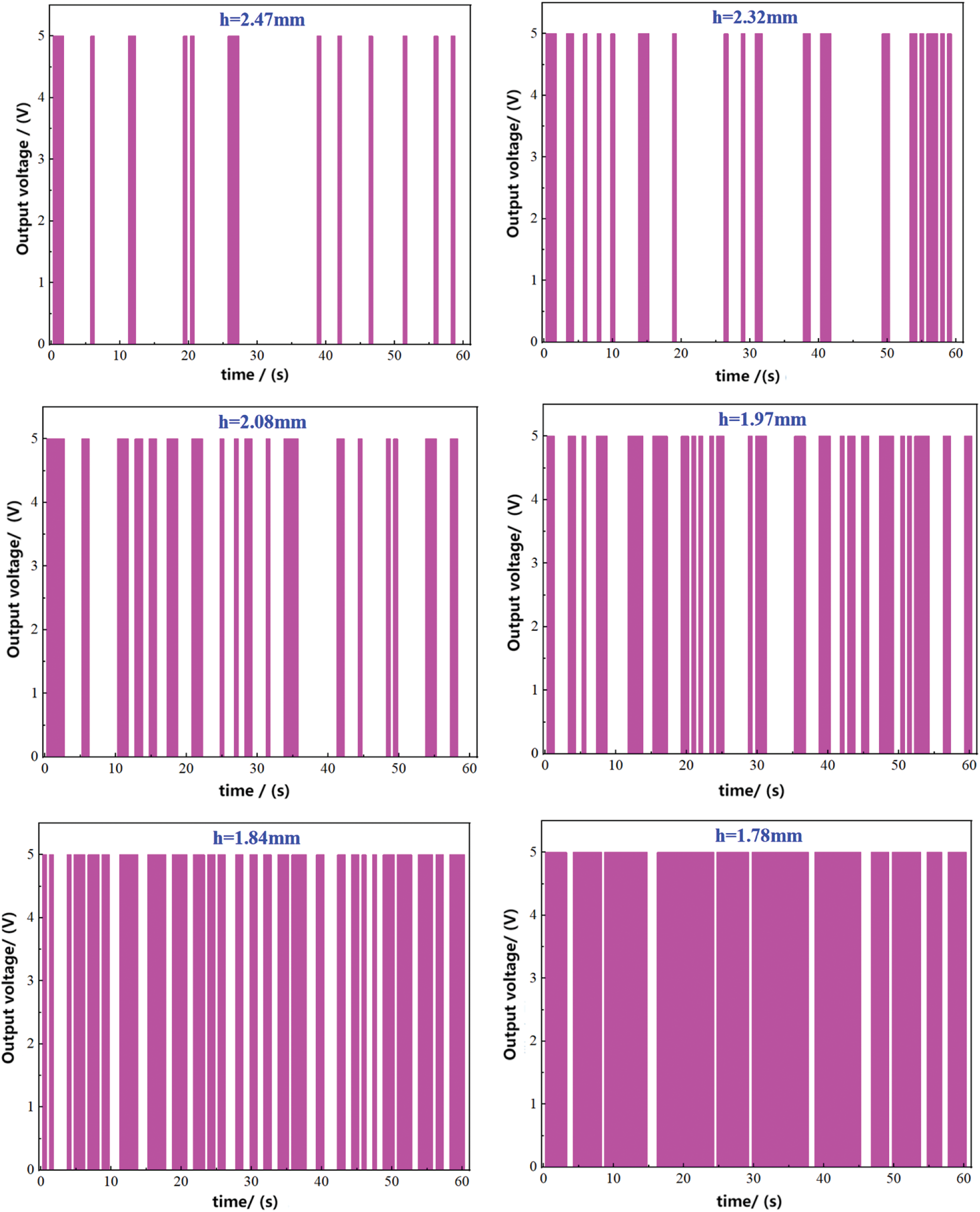
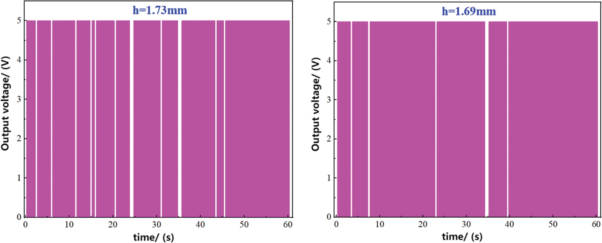
Figure 11: The measurement output signals at different heights (h)

Analysis of the results in Fig. 11 revealed that during the initial stage of high voltage output from the acquisition module, the duty cycle was relatively small. This could be attributed to the significant distance between the probe tip and the bottom of the pipe, allowing only a small portion of the liquid film peak region to make contact with the probe tip and establish electrical conductivity.

By continuously adjusting the movement distance of the automatic conductivity probe, the contact time between the probe tip and the bottom of the pipe decreased, resulting in an increased duration of contact between the probe tip and the liquid film within a fixed time interval. Consequently, an increase in the duty cycle of the high voltage value was observed, as depicted in Fig. 12. During the measurement process, occasional non-conduction phenomenon occurred due to the presence of a small amount of bubbles within the liquid film formed by the forced annular flow. Hence, when the duty cycle reached or exceeded 90%, it could be inferred that a stable liquid annulus had been established.

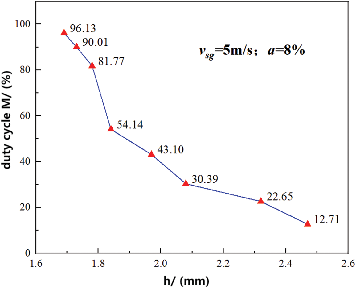
Figure 12: Duty cycle of high voltage values at different heights (h)

5.2 Analysis of Void Fraction Calculation Results

To assess the measurement results, the void fractions obtained in this study under various operating conditions were compared with the void fraction model proposed by Cioncolini and Thome [34], as depicted in Fig. 13. The prediction method in the Cioncolini model is simpler compared to most existing correlations, as it only depends on vapor quality and the gas to liquid density ratio, yet it reproduces the available data better than existing prediction methods. This comparison aimed to assess the accuracy of the measurements. The void fraction calculation model proposed by Cioncolini is expressed by Eq. (6), providing a theoretical basis for void fraction estimation.

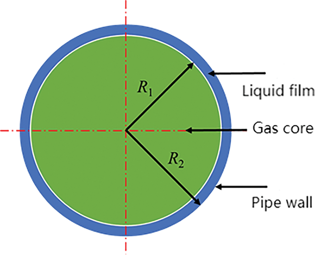
Figure 13: Schematic diagram of simplified liquid film in pipeline

ε=hxn1+(h−1)xn;0<x<1,10−3<ρgρl−1<1,0.7<ε<1 (6)

In the equation, ε represents the void fraction, x represents the gas phase mass fraction. In addition, parameters h and n are density ratio functions for the gas and liquid phases, and the functional expressions for parameters h and n are given by Eqs. (7) and (8).

h=−2.129+3.129(ρgρl−1)−0.2186 (7)

n=0.3487+0.5613(ρgρl−1)0.5150 (8)

In this study, the void fraction was calculated using the weighted average thickness algorithm for ten distinct operating conditions. The impact of maintaining a constant gas phase superficial velocity while altering the liquid phase volume fraction, as well as maintaining a constant liquid phase volume fraction while modifying the gas phase superficial velocity, was investigated. These results were then compared with the void fraction model proposed by Cioncolini. The outcomes of these comparisons are presented in Fig. 14, enabling a comprehensive evaluation of the measurement results in relation to the void fraction model.

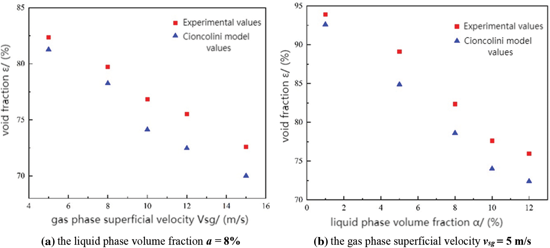
Figure 14: Comparison of measured void fractions under different operating conditions with values calculated by the Cioncolini model

Upon analyzing Fig. 14, it is evident that an increase in the gas phase superficial velocity while maintaining a constant gas-liquid ratio resulted in the gas phase carrying more liquid, leading to a reduction in the gas volume within the flow cross-section and a subsequent decrease in the void fraction. Conversely, when the gas phase superficial velocity was kept low and constant, gradually increasing the liquid phase volume fraction only yielded a minor decrease in the void fraction. This could be attributed to the limited gas volume flow rate and weak gas-liquid carrying capability. Despite the increase in the liquid phase volume fraction, the amount of liquid carried by the gas phase did not significantly increase, leading to a relatively small change in the void fraction. However, when the gas volume flow rate was sufficiently high, the gas-liquid carrying capacity intensified, resulting in a larger volume of separated liquid phase within the flow cross-section and consequently decreasing the void fraction.

Upon comparing of the experimental void fraction values obtained in this study with the void fraction values calculated by the Cioncolini model, a deviation was observed between the two scenarios, as illustrated in Fig. 15. This suggested that variations exist between the experimental and modeled void fraction values, highlighting the importance of further investigation and refinement of the measurement methodology.

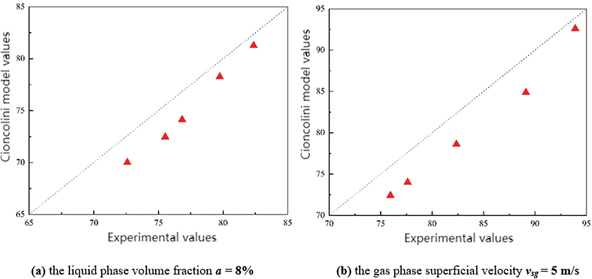
Figure 15: Deviation of measured void fractions under different operating conditions compared with values calculated by the Cioncolini model

Upon By examining the deviation plots, it was evident that the experimental void fraction values obtained in this study were higher than the values calculated by the Cioncolini model. However, the deviations for both scenarios remained within an acceptable range, with maximum deviations of 3.05% and 4.23%, respectively, and did not exceed 5%. This disparity could be attributed to the omission of the deviation caused by the swirling device in the void fraction calculation after measuring the liquid film thickness. The passage of the two-phase flow through the swirl device generated vigorous vortices, and the calculation process neglected factors such as centrifugal force, viscous force, and losses incurred by these vortices. Moreover, upon comparing the deviation plots of the void fraction, it was notable that the deviation values increased with higher gas phase superficial velocities. This was primarily due to the enhanced carrying capacity of the liquid phase by the higher gas phase velocities. However, the calculation process did not account for the liquid droplets carried by the gas core within the “film-core” structure formed by the forced annular flow. Consequently, a certain deviation existed between the actual measured void fraction values and the values calculated by the Cioncolini model.

6  Conclusion

(1) To address the limitations of traditional direct conductivity methods that can only statically measure void fraction in two-phase flows, a novel reciprocating dynamic conductivity sensor device based on forced annular flow was developed. This innovative device enabled remote online real-time measurement of liquid film thickness, offering a practical solution for void fraction measurement with significant engineering applicability.

(2) Through the analysis of experimental data and the utilization of the Cioncolini model, the calculated void fraction exhibited distinct trends. When maintaining a constant gas-liquid ratio at the device inlet, varying the gas phase superficial velocity revealed that as the gas superficial velocity increased, the gas phase gradually carried more liquid, resulting in a continuous reduction in the void fraction. Conversely, at a relatively low and constant gas superficial velocity, the void fraction experienced a minor decrease with increasing liquid phase volume fraction. However, when the gas volume flow rate was sufficiently high, the gas phase demonstrated enhanced liquid-carrying capabilities, leading to a notable decrease in void fraction as the separated liquid phase volume increased across the flow cross-section.

(3) In practical measurements, the influence of deviations induced by the swirl device is not considered when calculating void fraction. As a result, the experimental measurements of void fraction surpassed the values predicted by the Cioncolini model. Specifically, under conditions where the liquid phase volume fraction and gas phase superficial velocity remained constant, the maximum deviations between the experimental values and the Cioncolini model values were found to be 3.05% and 4.23%, respectively.

Acknowledgement: None.

Funding Statement: The authors would like to acknowledge the support provided by the National Natural Science Foundation of China (No. 62173049) and the Open Fund of the Hubei Key Laboratory of Oil and Gas Drilling and Production Engineering (Yangtze University), YQZC202309.

Author Contributions: The authors confirm contribution to the paper as follows: study conception and design: Xiaochu Luo, Xingkai Zhang; data collection: Xiaobing Qi, Zhao Luo; analysis and interpretation of results: Zhonghao Li, Ruiquan Liao; draft manuscript preparation: Xiaochu Luo, Xingkai Zhang. All authors reviewed the results and approved the final version of the manuscript.

Availability of Data and Materials: The authors acknowledge the importance of data accessibility in scientific research and strive to promote transparency and reproducibility. In this study, all data were obtained experimentally and presented in the form of data graphs in the article. However, it must be noted that there may be certain instances where data cannot be released due to legitimate reasons. These reasons may include legal or ethical restrictions, privacy concerns, intellectual property rights, or agreements with third parties. We assure you that any unavailability of data is not intended to hinder scientific progress but rather to ensure compliance with applicable regulations and protect the rights and privacy of individuals or entities involved. We thank our readers for their understanding and support in promoting open science while respecting the limitations and constraints associated with data accessibility. Should there be any concerns or inquiries regarding data availability, please feel free to contact us directly.

Conflicts of Interest: The authors declare that they have no conflicts of interest to report regarding the present study.

References

1. Zhang, L., Zhang, S. (2023). Analysis and identification of gas-liquid two-phase flow pattern based on multi-scale power spectral entropy and pseudo-image encoding. Energy, 282, 128835. https://doi.org/10.1016/j.energy.2023.128835 [Google Scholar] [CrossRef]

2. Fang, L. D., Yuan, X. Y., Zhang, Z. Y., Zhou, C., Li, H. L. et al. (2023). An eight-channel-based near infrared void fraction measurement system using T-ART algorithm. Optics and Lasers in Engineering, 161, 07385. [Google Scholar]

3. Shi, S. Q., Wang, Y. Q., Qi, Z. L., Yan, W. D., Zhou, F. Y. (2021). Experiment investigation and new void-fraction calculation method for gas-liquid two-phase flows in vertical downward pipe. Experimental Thermal and Fluid Science, 121, 110252. https://doi.org/10.1016/j.expthermflusci.2020.110252 [Google Scholar] [CrossRef]

4. Kawahara, A., Sadatomi, M., Nei, K., Matsuo, H. (2009). Experimental study on bubble velocity, void fraction and pressure drop for gas-liquid two-phase flow in a circular microchannel. International Journal Heat Fluid Flow, 30, 831–841. https://doi.org/10.1016/j.ijheatfluidflow.2009.02.017 [Google Scholar] [CrossRef]

5. Amiri, S., Ali, P. J. M., Mohammed, S., Hanus, R., Abdulkareem, L. et al. (2021). Proposing a nondestructive and intelligent system for simultaneous determining flow regime and void fraction percentage of gas-liquid two phase flows using polychromatic X-ray transmission spectra. Journal of Nondestructive Evaluation, 40(2), 47. https://doi.org/10.1007/s10921-021-00782-w [Google Scholar] [CrossRef]

6. Abro, E., Khoryakov, V. A., Johansen, G. A. (1999). Determination of void fraction and flow regime using a neural network trained on simulated data based on gamma-ray densitometry. Measurement Science &Technology, 10(7), 619–630. https://doi.org/10.1088/0957-0233/10/7/308 [Google Scholar] [CrossRef]

7. Faghihi, R., Nematollahi, M., Erfaninia, A., Adineh, M. (2015). Void fraction measurement in modeled two-phase flow inside a vertical pipe by using polyethylene phantoms. International Journal of Hydrogen Energy, 40(44), 15206–15212. https://doi.org/10.1016/j.ijhydene.2015.06.162 [Google Scholar] [CrossRef]

8. Nazemi, E., Roshani, G. H., Feghhi, S. A. H., Setayeshi, S., Zadeh, E. et al. (2016). Optimization of a method for identifying the flow regime and measuring void fraction in a broad beam gamma-ray attenuation technique. International Journal of Hydrogen Energy, 41, 7438–7444. https://doi.org/10.1016/j.ijhydene.2015.12.098 [Google Scholar] [CrossRef]

9. Khayat, O., Afarideh, H. (2019). Design and simulation of a multienergy gamma ray absorptiometry system for multiphase flow metering with accurate void fraction and water-liquid ratio approximation. Nukleonika, 64(1), 19–29. https://doi.org/10.2478/nuka-2019-0003 [Google Scholar] [CrossRef]

10. Hanus, R., Zych, M., Petryka, L., Jaszczur, M., Hanus, P. (2016). Signals features extraction in liquid-gas flow measurements using gamma densitometry. Part 1: Time domain. Epj Web of Conferences, 114, 02035. https://doi.org/10.1051/epjconf/201611402035 [Google Scholar] [CrossRef]

11. Antonenkov, D. A. (2021). Device for research of water flow dynamics in situ based on the PIV method. IOP Conference Series: Earth and Environmental Science, 666(2), 1755–1315. [Google Scholar]

12. García-Blanco, Y. J., Mancilla, E., Germer, E. M., Franco, A. T. (2021). A PIV investigation of laminar and turbulent viscoplastic fluid flow on axisymmetric abrupt contraction. Fluid Dynamics Research, 53(5), 1873–7005. [Google Scholar]

13. Tao, M. M., Jin, Y. L., Gu, N., Huang, L. (2010). A method to control the fabrication of etched optical fiber probes with nanometric tips. Journal of Optics, 12(1), 2040–8978. [Google Scholar]

14. Wang, F., Jin, N. D., Wang, D. Y., Han, Y. F., Liu, D. Y. (2017). Measurement of gas phase characteristics in bubbly oil-gas-water flows using bi-optical fiber and high-resolution conductance probes. Experimental Thermal & Fluid Science, 88, 361–375. https://doi.org/10.1016/j.expthermflusci.2017.06.017 [Google Scholar] [CrossRef]

15. Sardeshpande, M. V., Hanrinarayan, S., Ranade, V. V. (2015). Void fraction measurement using electrical capacitance tomography and high speed photography. Chemical Engineering Research & Design: Transactions of the Institution of Chemical Engineers, 94, 1–11. https://doi.org/10.1016/j.cherd.2014.11.013 [Google Scholar] [CrossRef]

16. Zhao, A., Han, Y. F., Zhang, H. X., Liu, W. X., Jin, N. D. (2016). Optimal design for measuring gas holdup in gas-liquid two-phase slug flow using quick closing valve method. CIESC Journal, 67(4), 1159–1168 (In Chinese). [Google Scholar]

17. Kim, J., Ahn, Y. C., Kim, M. H. (2009). Measurement of void fraction and bubble speed of slug flow with three-ring conductance probes. Flow Measurement and Instrumentation, 20(3), 103–109. https://doi.org/10.1016/j.flowmeasinst.2009.02.001 [Google Scholar] [CrossRef]

18. Nassos, G. P., Bankoff, S. G. (1967). Local resistivity probe for study of point properties of gas-liquid flows. The Canadian Journal of Chemical Engineering, 45(5), 271–274. https://doi.org/10.1002/cjce.v45:5 [Google Scholar] [CrossRef]

19. Lv, Y. L., Chen, Z. Y., Du, S. W., He, L. M. (2003). Measurement of cavitation rate in gas-liquid two-phase flow with conductance probe. Industrial Metrology, 2003(S1), 208–211. [Google Scholar]

20. Devia, F., Fossa, M. (2003). Design and optimisation of impedance probes for void fraction measurements. Flow Measurement and Instrumentation, 14(4–5), 139–149. [Google Scholar]

21. Fossa, M., Guglielmini, G., Marchitto, A. (2003). Intermittent flow parameters from void fraction analysis. Flow Measurement and Instrumentation, 14, 161–168. https://doi.org/10.1016/S0955-5986(03)00021-9 [Google Scholar] [CrossRef]

22. Sun, X., Kuran, S., Ishii, M. (2004). Cap bubbly-to-slug flow regime transition in a vertical annulus. Experiments in Fluids, 37(3), 458–464. https://doi.org/10.1007/s00348-004-0809-z [Google Scholar] [CrossRef]

23. Ito, D., Kikura, H., Aritomi, M. (2011). Micro wire-mesh sensor for two-phase flow measurement in a rectangular narrow channel. Flow Measurement and Instrumentation, 22(5), 377–382. https://doi.org/10.1016/j.flowmeasinst.2011.06.001 [Google Scholar] [CrossRef]

24. Ko, M. S., Lee, S. Y., Lee, B. A., Yun, B. J., Kim, K. Y. et al. (2013). An electrical impedance sensor for water level measurements in air-water two-phase stratified flows. Measurement Science and Technology, 24(9), 95301. https://doi.org/10.1088/0957-0233/24/9/095301 [Google Scholar] [CrossRef]

25. Ko, M. S., Lee, B. A., Won, W. Y., Lee, Y. G., Jerng, D. W. et al. (2015). An improved electrical conductance sensor for void-fraction measurement in a horizontal pipe. Nuclear Engineering & Technology, 47(7), 804–813. https://doi.org/10.1016/j.net.2015.06.015 [Google Scholar] [CrossRef]

26. Lee, Y. G., Won, W. Y., Lee, B. A., Kim, S. (2017). A dual conductance sensor for simultaneous measurement of void fraction and structure velocity of downward two-phase flow in a slightly inclined pipe. Sensors, 17(5), 1063. [Google Scholar] [PubMed]

27. Xu, Y., Xie, F., Li, J., Zhang, T., Li, T. et al. (2018). A capacitance sensor with hydrocyclone phase separator for measuring water volume fraction in gas-liquid two-phase flow. CIESC Journal, 69(4), 1357–1364 (In Chinese). [Google Scholar]

28. Wei, P. K., Wang, D., Niu, P. M., Pang, C. K., Liu, M. (2020). A novel centrifugal gas liquid pipe separator for high velocity wet gas separation. International Journal of Multiphase Flow, 124, 103190. https://doi.org/10.1016/j.ijmultiphaseflow.2019.103190 [Google Scholar] [CrossRef]

29. Niu, P. M., Wang, D., Yang, Y., Wei, P. K., Pan, Y. Z. et al. (2019). Void fraction measurement using an imaging and phase isolation method in horizontal annular flow. Measurement Science and Technology, 30(2), 1361–6501. [Google Scholar]

30. Li, Z. H., Zhang, X. K., Liao, R. Q., Shi, B. C., Hang, L. M. (2022). Research on liquid holdup measurement by conductivity method based on forced annular flow. China Petroleum Machinery, 50(4), 101–110. [Google Scholar]

31. Ghendour, N., Azzi, A., Meribout, M., Zeghloul, A. (2021). Modeling and design of a new conductance probe for gas void fraction measurement of two-phase flow through annulus. Flow Measurement and Instrumentation, 82, 102078. https://doi.org/10.1016/j.flowmeasinst.2021.102078 [Google Scholar] [CrossRef]

32. Chen, C. (2017). Research on conductivity probe sensor for horizontal annular flow liquid film measurement (Master Thesis). Tianjin University, China. [Google Scholar]

33. Guo, J., Wang, X. D., Zhang, X. K., Yang, M. (2020). Phase separation characteristics of gas-liquid two-phase flow with high gas-liquid ratio in pipeline. Journal of Xi’an Shiyou University (Natural Science Edition), 35(5), 77–82+115 (In Chinese). [Google Scholar]

34. Cioncolini, A., Thome, J. R. (2012). Void fraction prediction in annular two-phase flow. International Journal of Multiphase Flow, 43, 72–84. https://doi.org/10.1016/j.ijmultiphaseflow.2012.03.003 [Google Scholar] [CrossRef]